The Sunyaev-Zeldovich effect in superclusters of galaxies using gasdynamical simulations: the case of Corona Borealis

Abstract

We study the thermal and kinetic Sunyaev–Zel’dovich (SZ) effect associated with superclusters of galaxies using the MareNostrum Universe SPH simulation. In particular, we consider superclusters with characteristics (total mass, overdensity and number density of cluster members) similar to those of the Corona Borealis Supercluster (CrB-SC). This paper is motivated by the detection at 33 GHz of a strong temperature decrement in the cosmic microwave background towards the core of this supercluster (Génova-Santos et al. 2005, 2008). Multifrequency observations with VSA and MITO suggest the existence of a thermal SZ effect component in the spectrum of this cold spot, with a Comptonization parameter value of $y=7.8^{+4.4}_{-5.3}\times 10^{-6}$ (Battistelli et al. 2006), which would account for roughly 25 per cent of the total observed decrement.

From the SPH simulation, we identify nine $(50$ $~{}{\rm h}^{-1}~{}{\rm Mpc})^{3}$ regions containing superclusters similar to CrB-SC, obtain the associated SZ maps and calculate the probability of finding such SZ signals arising from hot gas within the supercluster. Our results show that the Warm–Hot Intergalactic Medium (WHIM) lying in the intercluster regions within the supercluster produces a thermal SZ effect much smaller than the observed value by MITO/VSA.

Neither can summing the contribution of small clusters and galaxy groups ($M<5\times 10^{13}$ $~{}{\rm h}^{-1}~{}{\rm M}_{\odot}$) in the region explain the amplitude of the SZ signal. Our synthetic maps show peak $y$-values significantly below the observations. Less than 0.3% are compatible at the lower end of the 1-sigma level, even when considering privileged orientations in which the filamentary structures are aligned along the line of sight. When we take into account the actual posterior distribution from the observations, the probability that WHIM can cause a thermal SZ signal like the one observed in the CrB-SC is $<1\%$, rising up to a $3.2\%$ when the contribution of small clusters and galaxy groups is included. If the simulations provide a suitable description of the gas physics, then we must conclude that the thermal SZ component of the CrB spot most probably arises from an unknown galaxy cluster along the line of sight. On the other hand, the simulations also show that the kinetic SZ signal associated with the supercluster cannot provide an explanation for the remaining 75% of the observed cold spot in CrB.

1 Introduction

A detailed account of the baryons present in all known components of the local Universe gives a value for the baryon density parameter of $\Omega_{\rm B}=(0.010\pm 0.003)h^{-2}$ (see e.g. Fukugita et al., 1998)). Primordial nucleosynthesis (Burles et al., 2001), observations of the Lyman-$\alpha$ forest (Rauch et al., 1997) and measurements of the angular power spectrum of the Cosmic Microwave Background (CMB, Rebolo et al., 2004; Spergel et al., 2007) lead to values two times higher for this parameter. It seems that there must exist a baryonic component in the local Universe where half of the baryons would remain hidden. Theoretical models (e.g. Cen & Ostriker, 1999) based on gasdynamical simulations suggest that these missing baryons could be accounted for in a diffuse gas phase with temperatures $10^{5}<T<10^{7}$K and moderate overdensities ($\delta\la 10-100$), known as the ‘warm/hot intergalactic medium’ (WHIM). According to these simulations, the WHIM would be located in filaments connecting clusters of galaxies and in large-scale sheet-like structures. The existence of the WHIM component is a fairly robust conclusion against changes in the gas physics included in the simulations, as feedback processes (see e.g. Cen & Ostriker, 2006). It has been shown that even when considering nonequilibrium for major metal species, UV photoionization and galactic superwinds, the fraction of baryons in the form of WHIM is still of order

There is observational evidence of this WHIM component, using absorption lines in the spectra of background sources, either in ultraviolet wavelengths for the lower temperature WHIM (e.g. Savage et al., 1998; Nicastro et al., 2003), or in the X-ray range (first claimed detection by Nicastro et al. (2005) towards Mkn 421, although it is still under discussion; recently detected by Buote et al. (2009) towards the Sculptor Wall). Apart from this possibility, the WHIM could also be detected via inverse Compton scattering of CMB photons, the so-called Sunyaev-Zel’dovich (SZ) effect (Sunyaev & Zeldovich, 1972). In this work we focus on this physical process and study both the thermal (tSZ) and kinetic (kSZ) signals associated with this gas phase. The SZ effect was first proposed for clusters of galaxies and has since been proven to be an extremely useful tool for studying cluster physics. When combining SZ measurements with X-ray and/or optical measurements it is possible to obtain an independent determination of the cosmological parameters (Carlstrom et al., 2000). Recently, it has also been proven that SZ surveys are effective means of finding new galaxy clusters in blind surveys (Staniszewski et al., 2008).

Although the SZ effect has only been observed robustly in the direction of clusters of galaxies (for a review see Birkinshaw, 1999), the aforementioned simulations by Cen & Ostriker (1999) and other theoretical models (Persic et al., 1988; Persic et al., 1990; Boughn, 1999) suggest that SZ surveys in superclusters could lead to a detection of the WHIM. The basic idea is that since the SZ effect is proportional to the line-of-sight integral of the electron pressure, filamentary structures of superclusters extending over several tens of megaparsecs could overcome the expected low baryon overdensities and produce a measurable signal with present-day observing facilities. Following these ideas, Atrio-Barandela & Mücket (2006) theoretically computed the expected SZ anisotropies associated with this WHIM phase and found its dependence on gas and cosmological parameters. Moreover, and based on numerical simulations, Dolag et al. (2005); Hansen et al. (2005); Hernández-Monteagudo et al. (2006) and Roncarelli et al. (2007) have provided coinciding predictions of the contribution of diffuse (non-collapsed) gas to the thermal SZ power spectrum. In particular, Hallman et al. (2007) concluded that the contribution from unbound gas could be as high as 12% that of galaxy clusters.

Observations of the Corona Borealis (CrB) supercluster carried out with the extended configuration (11 arcmin resolution) (Watson et al., 2003) of the Very Small Array (VSA) at 33 GHz (Genova-Santos et al., 2005) showed the existence of two strong and resolved negative features in a region where there are no known clusters of galaxies. Our study focuses on the strongest spot, the so-called “H-spot”, which has a temperature decrement of $\Delta T=-230\pm 23~{}\mu$K. This region is in fact the most negative feature found in any of the maps produced by the VSA, which in total covered a sky area of $\sim 100$ deg². Moreover, a detailed Gaussianity study in the region (Rubiño-Martín et al., 2006) finds a clear deviation (99.82%) at angular scales of multipole $\ell\sim 500$. Génova-Santos et al. (2008) have recently presented new VSA observations with an equivalent angular resolution of 6 arcmin that confirm the existence of the “H-spot”.

The origin of the CrB spot is still unclear. Among other options, a possible explanation could be an SZ effect. Observations performed with the MITO (Millimetre & Infrared Testa Grigia Observatory) telescope (De Petris et al., 1999) at 143, 214 and 272 GHz and an angular resolution of 16 arcmin showed that roughly 25% of the total signal has a thermal SZ spectral behaviour, yielding a Comptonization parameter of $y=7.8^{+4.4}_{-5.3}\times 10^{-6}$ at 68% C.L. (Battistelli et al., 2006; Battistelli et al., 2007). Summarizing, we need to find an explanation for this tSZ component, but we also need to understand the origin of the remaining $\sim 75$% of the cold spot: even when removing the detected tSZ signal, the CrB-H decrement is a $3.9\sigma$ deviation with respect to Gaussianity.

In this paper, we use numerical simulations to explore the possibility that the signal observed in the CrB-H spot originates by diffuse gas (WHIM) within the supercluster. Basically, we want to test whether or not the MNU simulations are able to explain the detected tSZ signal by MITO/VSA in terms of the WHIM. Additionally, we test whether the same WHIM component can provide a relevant contribution to the total decrement in terms of its kinetic SZ effect. N-body numerical gasdynamical simulations have proved a very useful tool in establishing accurate theoretical predictions of the SZ signals induced either by galaxy clusters or the WHIM component (see e.g. Da Silva et al., 2000; Springel et al., 2001; Dolag et al., 2005; Hansen et al., 2005; Hernández-Monteagudo et al., 2006; Roncarelli et al., 2007; Hallman et al., 2007, 2009). However, these studies have mainly focused on the statistical properties of these signals (e.g. predictions for the SZ angular power spectrum, or the one-point probability distribution function of the full sky maps as a whole). In this study, we restrict our analyses to superclusters and we study the probability of finding spots produced by SZ signals such as those observed in CrB. In addition, we also provide predictions for the observability of those individual features in the maps produced by the the next generation of instruments, such as the Planck satellite (The Planck Collaboration, 2006).

In §2 we briefly describe the main characteristics of the simulations used; in §3 a complete description of the methodology applied in the study is given, and in §4 we present a general statistic description of the maps. In §5 we present our main analysis for the particular case of the CrB-SC spot while in §6 we provide an estimate of the observability of SZ signals with Planck. Finally, in §7 we present a discussion and our conclusions obtained with this study.

2 Simulations

For the analysis reported in this paper we have used the MareNostrum Universe (hereafter MNU) SPH simulation, which is currently the largest cosmological N-body+SPH simulation carried out so far. It consists of $1024^{3}$ dark and $1024^{3}$ SPH particles in a cubic computational volume of $500~{}{\rm h}^{-1}~{}{\rm Mpc}$ on a side. This simulation was done at the MareNostrum supercomputer, from which it took the name, located at the Barcelona Supercomputer Center, Centro Nacional de Supercomputación (BSC-CNS). Initial conditions were set up according to the so-called “Concordance $\Lambda$-CDM Model” with parameters $\Omega_{\rm m}=0.3$, $\Omega_{\Lambda}=0.7$, $\Omega_{\rm b}=0.045$, $\sigma_{8}=0.9$ and $H_{0}=70$ km s^-1 Mpc^-1 and a slope of $n=1$ for the initial power spectrum (see Gottlöber & Yepes (2007) and Yepes et al. (2007) for more details of this simulation).

The mass of each dark matter particle is $m_{\rm DM}=8.239\times 10^{9}~{}{\rm h}^{-1}~{}{\rm M}_{\odot}$ and the mass of each gas particle is $m_{\rm gas}=1.454\times 10^{9}~{}{\rm h}^{-1}~{}{\rm M}_{\odot}$, evolved from redshift $z=40$ using the TREEPM+SPH code GADGET-2 (Springel et al., 2001; Springel, 2005). The spatial force resolution is set to an equivalent Plummer gravitational softening of $15$ h^-1 kpc, and the SPH smoothing length is set to the 40th neighbour to each particle.

We focused our work on the snapshot corresponding to redshift $z=0$, for which complete catalogues of objects are available, as described in the next subsection. Finally, to investigate the dependence of the results on the mass and spatial resolutions of the simulations, we have also considered a re-simulation of the same snapshot using identical initial conditions but with $2\times 256^{3}$ particles, which are also equally distributed between gas and dark matter, with $m_{\rm gas}=8.065\times 10^{10}$ $~{}{\rm h}^{-1}~{}{\rm M}_{\odot}$ and $m_{\rm DM}=5.397\times 10^{11}$ $~{}{\rm h}^{-1}~{}{\rm M}_{\odot}$. The same halo catalogues were available for this lower resolution simulation.

2.1 Halo identification algorithms

In order to find all structures and substructures within the distribution of 2 billion particles and to determine their properties we have used two different algorithms: a friends-of-friends analysis and a spherical overdensity halo-finder. We have started with the parallel version of the hierarchical friends-of-friends (FOF) algorithm (Klypin et al., 1999). We use a basic linking length of 0.17 of the mean interparticle separation to extract the FOF objects at redshift $z=0$. With this linking length we have identified more than 2 million objects with more than 20 DM particles which closely follow a Sheth-Tormen mass function (Gottlöber et al., 2006). More than 4000 galaxy clusters with masses larger than $10^{14}~{}{\rm h}^{-1}~{}{\rm M}_{\odot}$ have been found. If one divides this linking length by $2^{n}$ ($n=1,3$) substructures and in particular the centres (density peaks) of the objects can be identified.

Spherical halos are identified using the AMIGA-Halo-Finder (AHF) (Knollmann & Knebe, 2009), an MPI parallelized modification of the algorithm presented in Gill et al. (2004). The halo finder locates halos (as well as subhalos) as peaks in an adaptively smoothed density field. The local potential minima are computed for each peak and within spherical volumes the set of particles that are gravitationally bound to the peak is determined. If the peak contains more than 20 particles, then its virial (or truncation) radius is calculated. The virial radius $R_{\rm vir}$ is the point at which the density profile drops below the virial overdensity $M(<R_{\rm vir})/(4\pi R_{\rm vir}^{3}/3)=\Delta_{\rm vir}\rho_{\rm mean}$, where $\Delta_{\rm vir}$ depends on the cosmology (Kitayama & Suto, 1996); in our case, $\Delta_{\rm vir}=330$. However, for subhalos this prescription is not appropriate. Subhalos exist in the dense environment of their host halo, where the density exceeds the virial one. In this case the density profile shows a characteristic upturn. This is the truncation radius of the the subhalo. We have checked that the number of halos found in our simulations is basically the same when using the FOF and AHF algorithms.

These two catalogues (FOF and AHF) have been used as a tool to identify the regions of interest and to separate the contribution to the SZ signal of galaxy clusters from that of the diffuse gas, as we explain in §3.

3 Methodology

To characterize the statistical properties of the SZ signals associated with superclusters of galaxies similar to the CrB, we proceed the following way. We first identify specific regions (superclusters) within the whole MNU simulation, which are selected to have similar characteristics (in terms of total mass, overdensity and number density of cluster objects) to those of CrB. All our analyses are focused on these particular regions. Once these “mock CrB regions” are identified, we produce the associated SZ maps (both thermal and kinetic components), provided that these regions are placed at the distance of CrB, using an average redshift for the supercluster of $z=0.07$ (Genova-Santos et al., 2005), and the cosmological parameters of the simulation.

In order to isolate the contribution of the different physical components to these maps, we produce five sets of maps, considering: (a) all gas particles; (b) all gas particles except those which are associated with clusters in the region; (c) only WHIM particles, defined as those gas particles having temperatures within the range $10^{5}$ to $10^{7}$ K; (d) only gas particles that belong to the clusters; and (e) only gas particles that belong to groups of galaxies. The last three sets of maps complement each other in the sense that their sum is equal to the map for case (a). Finally, and in order to explore the dependence of the amplitude of the detected signals with the relative orientation of the supercluster, we have also produced sets of SZ maps using random orientations of the simulation box with respect to the observer for all the sets of maps described above.

All these steps are described in the following subsections.

3.1 Identification of superclusters similar to CrB

The Corona Borealis supercluster (CrB-SC) has been morphologically described by Small et al. (1997) as a flattened pancake of $100~{}{\rm h}^{-1}~{}{\rm Mpc}$ a side with an estimated depth of $40~{}{\rm h}^{-1}~{}{\rm Mpc}$. According to the catalogue by Einasto et al. (2001), it includes eight clusters with total masses (including gas and dark matter) ranging from $1.5\times 10^{14}\rm M_{\odot}$ to $8.9\times 10^{14}\rm M_{\odot}$, yielding a total mass for the supercluster of $(3-8)\times 10^{16}\rm M_{\odot}$ (Genova-Santos et al., 2005). However, the core of the supercluster, where the Abell clusters lie, extends over an area of only $20~{}{\rm h}^{-1}~{}{\rm Mpc}$ a side. Hence, we decided to study cubic subvolumes of $50~{}{\rm h}^{-1}~{}{\rm Mpc}$ a side, which were identified as similar to CrB-SC by using the two independent criteria described below:

• Criterion 1: Over-densities. Assuming that the CrB supercluster is spherically symmetrical and all its mass is concentrated in the core, its average density would be of the order of $1.67\times 10^{12}~{}{\rm h}^{-1}~{}{\rm M}_{\odot}(~{}{\rm h}^{-1}~{}{\rm Mpc})^{-3}$. The average density of the simulation is of the order of $8.33\times 10^{10}~{}{\rm h}^{-1}~{}{\rm M}_{\odot}(~{}{\rm h}^{-1}~{}{\rm Mpc})^{-3}$, calculated by dividing the total mass (DM + gas) between the volume of the simulation. Thus, it is around 20 times smaller than the CrB average density. Given this fact, an overdensity criterion for the gas particles in the simulation can be used in order to locate CrB-like regions.

  We considered as candidate regions the subvolumes of $50~{}{\rm h}^{-1}~{}{\rm Mpc}$ a side that contained the largest number of overdense gas particles, i.e. gas particles which show a density larger than or equal to $20$ times the average density of the simulation. These regions are guaranteed to have a similar overdensity to that of CrB supercluster and enough gas particles within to allow further filtering when building the different sets of maps.

• Criterion 2: Resemblance to CrB. The number of clusters and the total mass within a given subvolume were the two characteristics considered in order to apply this criterion. A complete catalogue of the objects present in the simulation and their masses was required.

  A subvolume of $50~{}{\rm h}^{-1}~{}{\rm Mpc}$ a side was considered as a candidate for the study when it satisfied 1) baryonic mass of the order of the mass of the CrB supercluster, i.e. $M_{\rm gas}\geq 10^{15}$ $~{}{\rm h}^{-1}~{}{\rm M}_{\odot}$; and 2) the number of clusters within is greater or equal to 6, defining a cluster as an object with $M_{\rm Total}=M_{\rm gas}+M_{\rm DM}\geq 5\times 10^{13}$ $~{}{\rm h}^{-1}~{}{\rm M}_{\odot}$. Therefore, this criterion established minimum thresholds for the total mass of the candidate regions, the number of clusters within and the mass of these clusters. Note that, in order to be conservative, these three thresholds lie below those of the CrB supercluster.

Table 1: Sub-volumes considered in this study. Each corresponds to a cubic box of 50 $~{}{\rm h}^{-1}~{}{\rm Mpc}$ a side. Columns 2 and 3 indicate the gas and total (dark+baryonic) mass within each subvolume. The last column indicates the number of clusters identified in the box using the AHF algorithm (see text for details).

Subvol.	$M_{\rm gas}$	$M_{\rm Total}$	No. clusters
	[$~{}{\rm h}^{-1}~{}{\rm M}_{\odot}$]	[$~{}{\rm h}^{-1}~{}{\rm M}_{\odot}$ ]	$M\geq 5\times 10^{13}~{}{\rm h}^{-1}~{}{\rm M}_{\odot}$
001	$2.29\times 10^{15}$	$1.53\times 10^{16}$	14
002	$2.30\times 10^{15}$	$1.54\times 10^{16}$	13
003	$2.01\times 10^{15}$	$1.34\times 10^{16}$	11
004	$2.94\times 10^{15}$	$1.96\times 10^{16}$	27
005	$1.90\times 10^{15}$	$1.27\times 10^{16}$	12
006	$2.45\times 10^{15}$	$1.63\times 10^{16}$	14
007	$2.85\times 10^{15}$	$1.91\times 10^{16}$	19
008	$2.74\times 10^{15}$	$1.83\times 10^{16}$	23
009	$2.85\times 10^{15}$	$1.90\times 10^{16}$	21

Nine sub-volumes were finally selected and are listed in Table 1. All regions satisfy the two aforementioned criteria, and are centred around the largest concentration of over-dense particles within each of them. None of the nine sub-volumes overlaps another. The last column in the table shows the total number of galaxy clusters (defined as halos with $M\geq 5\times 10^{13}$ $~{}{\rm h}^{-1}~{}{\rm M}_{\odot}$), which were taken from the AHF catalogue.

3.2 Building SZ maps

For each gas particle $i$, the simulation provides the position ($\mathbf{r}_{\rm i}$), velocity ($\mathbf{v}_{\rm i}$), temperature ($T_{\rm i}$), density ($\rho_{\rm i}$) and SPH smoothing length ($h_{\rm i}$). Using the physical parameters for all the particles, we can build the SZ maps following the procedure described in Da Silva et al. (2000). Each gas particle has an associated mass profile given by $m_{\rm gas}\ W(\mathbf{r}-\mathbf{r_{i}},h_{i})$, where $\mathbf{r}$ is the coordinate vector of the position in which we are calculating the mass profile, $\mathbf{r_{i}}$ is the coordinate vector of the position of the i-th gas particle, $h_{i}$ is the smoothing length for that particle and $W$ is the normalized spherically symmetric kernel adopted in the simulations, which in our case is given by (Springel et al., 2001):

$$W(x,h_{i})=\dfrac{8}{\pi h_{i}^{3}}\left\{\begin{array}[]{ll}1-6x^{2}+6x^{3},&0\leq x\leq 0.5\\ 2(1-x)^{3},&0.5<x\leq 1\\ 0,&x>1\end{array}\right.$$ (1)

where $x=|\mathbf{r}-\mathbf{r_{i}}|/h_{i}$. Thus, each particle occupies a sphere with a radius equal to its SPH smoothing length.

The thermal component of the SZ effect (tSZ) in a certain direction is given by the Comptonization $y$ parameter:

$$y=\int n_{e}\dfrac{k_{B}T_{e}}{m_{e}c^{2}}\sigma_{T}dl$$ (2)

where the integral is taken along the line of sight (los), $\sigma_{T}$ is the Thomson cross-section, $n_{e}$ is the electron number density, $T_{e}$ is the electronic temperature, $k_{B}$ is the Boltzmann constant and $m_{e}c^{2}$ is the electron rest mass energy. The numerical evaluation of the integral in Eq. 2 is done by discretizing the los integral as

$$y\simeq\frac{k_{B}\sigma_{T}}{m_{e}c^{2}}\frac{m_{\rm gas}}{\mu_{\rm e}m_{\rm p}}\Delta x\sum_{\alpha}\sum_{i}T_{i}W(|\mathbf{r_{\alpha}}-\mathbf{r_{i}}|,h_{i})$$ (3)

where $\Delta x$ is the discrete cell size along the los. In this equation, the $\alpha$ index runs over all the cells along the line of sight, the $i$ sum runs over all the particles that contribute to the column of cells projected onto a pixel, $\mu_{\rm e}$ is the electron mean molecular weight and $m_{\rm p}$ is the proton mass.

To build the tSZ maps, we make a further approximation, which consists in assuming a plane–parallel projection of the simulation boxes. At the distance of CrB, the error of using this approximation instead of doing the exact los integration is very small, as discussed below. Thus, for building the maps we create a 3D cubic grid with a cell size of $\Delta x=80h^{-1}kpc$ a side and we use equation 3 to obtain the Comptonization parameter for each cell.

A similar method is applied for the kinetic component of the SZ effect, given by the $b$-parameter

$$b=-\int n_{e}\frac{v_{\rm p}}{c}\sigma_{T}dl$$ (4)

where $v_{\rm p}=\vec{v}\cdot\hat{n}$ is the peculiar velocity of the cluster projected along the line of sight ($\hat{n}$), and $c$ is the speed of light. This equation is accordingly rewritten as

$$b\simeq\frac{\sigma_{T}}{c}\frac{m_{\rm gas}}{\mu_{\rm e}m_{\rm p}}\Delta x\sum_{\alpha}\sum_{i}v_{\rm p,\it i}W(|\mathbf{r_{\alpha}}-\mathbf{r_{i}}|,h_{i})$$ (5)

This process was carried out for each subvolume, yielding $y$ and $b$ maps with a pixel size of $\Delta x=80h^{-1}kpc$. This physical length is equivalent to an angular resolution of $1.4$ arcmin if we place the boxes at the CrB supercluster distance (using the redshift $z=0.07$ and the cosmological parameters of the simulation). These maps are then degraded in resolution, by a convolution with the appropriate Gaussian beam, in order to make predictions at the relevant angular resolutions. In particular, for the case of MITO/VSA, the maps are degraded to an angular resolution of $16^{\prime}$.

Examples of SZ maps for one of the subvolumes with $1.4^{\prime}$ resolution are shown in Figure 1, where it can be seen that the peak values match those of typical clusters of galaxies, i.e. $y_{\rm max}\sim 10^{-4}$ and $|b|_{\rm max}\sim 10^{-5}$. When comparing these numbers with other results from numerical simulations (e.g. Da Silva et al., 2000; Springel et al., 2001), it is important to take into account the effect of pixel scale, which in our case is significantly larger. Following Roncarelli et al. (2007), Figure 2 presents the distribution of the pixel values for the whole set of nine maps, in the plane of Doppler $|b|$ parameter versus $y$ parameter. Note that in our case, we are integrating the SZ flux only from a $50$ $~{}{\rm h}^{-1}~{}{\rm Mpc}$ region because we want to isolate the effect from the superclusters, and thus the peak of this distribution is shifted towards low values of $y$ parameter.

Figure 3 shows the effect of the beam convolution on the original map (Fig. 1), for the case of VSA/MITO resolution ($16^{\prime}$). The average $y$ parameter in the maps with clusters and a resolution of $1.4^{\prime}$ ranges from $0.73\times 10^{-7}$ to $1.3\times 10^{-7}$, the mean value being $<y>=9.6\times 10^{-8}$. Note that this result is roughly an order of magnitude lower than the average value of $\left\langle y\right\rangle=2.6\times 10^{-6}$ found by Springel et al. (2001). The reason is again that in our case, we are only integrating a total depth of 50 $~{}{\rm h}^{-1}~{}{\rm Mpc}$, while in their computations they consider all the integrated contribution up to $z=6$.

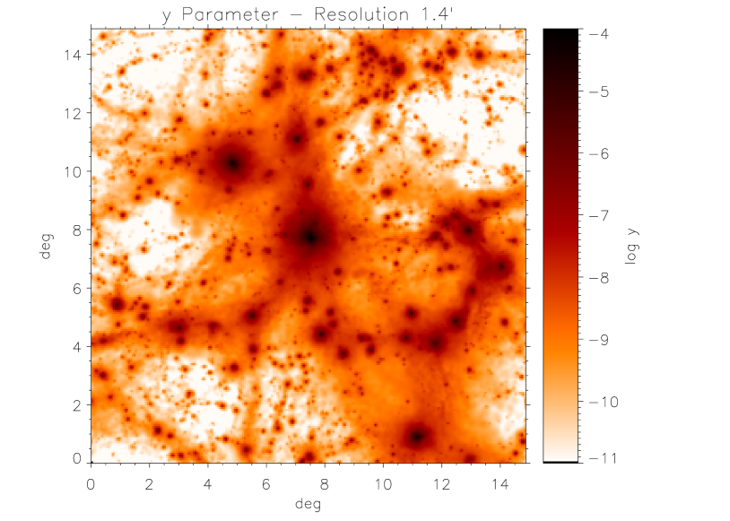
Figure 1: Example of Sunyaev–Zel’dovich effect maps obtained from the simulations. The angular resolution of the maps is $1.4^{\prime}$. Top: thermal SZ effect, given by the y-parameter map in logarithmic scale. Bottom: kinetic SZ effect, given by the logarithm of the absolute value of the $b$ parameter.

Figure 2: Two-dimensional distribution of the pixel values for the set of nine simulated maps in supercluster regions. The two axes represent the $y$ Compton parameter and the (modulus of the) $b$ parameter. Contour levels enclose the regions with 50, 70, 90 and 99.9 per cent of the total amount of pixels, respectively.

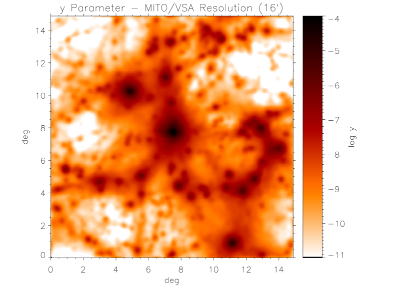
Figure 3: Comptonization parameter (on a logarithmic scale) of the same map shown in the top panel of figure 1, convolved with a Gaussian beam to match MITO/VSA resolution (16 arcmin).

The approach described above makes use of two approximations: a plane–parallel projection and approximate integral. To explore their validity, we have analytically obtained the profile for one single particle and we compared it to the one obtained using our map-mapping technique. This comparison yields a point-by-point difference in the profile of less than $5\%$ when the particle is located in the centre of the map and of less than $10\%$ when it is placed at a distance of $\sim 4^{\circ}$ along the diagonal of the subvolume. Both the integrated value and the maximum value show even smaller differences ($\leqslant 3\%$) when compared to the theoretical approach. We find that, in that case, the error in the central angular coordinate of a particle is smaller that the size of one pixel in our integration scheme.

3.3 Subtraction of galaxy clusters contribution to the maps

In order to characterize the SZ signal which is not associated with galaxy clusters in the subvolumes, the contribution of those particles which belong to clusters is eliminated from the los integration to produce a set of SZ maps that will contain only the contribution of WHIM and galaxy groups. In practice, two assumptions are needed to perform these computations. First, we have to adopt a definition of which halos are going to be considered as “galaxy clusters”, and thus they will be removed from the maps. In this study, we shall define clusters as those objects more massive than $5\times 10^{13}~{}{\rm h}^{-1}~{}{\rm M}_{\odot}$ (in total mass). This cluster mass threshold does not significantly alter our results. We note that those halos can be easily identified in any of the two catalogues described in §2.1.

Secondly, we need to specify to what extent we are removing particles from a given halo. A reasonable assumption is to remove those particles lying within one virial radius ($r_{\rm vir}$) from the cluster. Estimates for the virial radius of the clusters are provided in the AHF catalogue, so we shall adopt those values for this purpose. Using the $r_{\rm vir}$ values adopting the mass limit of galaxies of $M\geq 5\times 10^{13}\rm~{}{\rm h}^{-1}~{}{\rm M}_{\odot}$, clusters were extracted by using a spherical top-hat function; i.e. neglecting the contribution of every particle that lies within the virial radius of any given cluster (in the 3D grid).

3.4 Rotations

Gas in the WHIM phase is located mainly along filaments and sheet-like structures. Because the SZ effect probes the integral contribution of the electron pressure along the line of sight, we might expect certain orientations in which the gas in filaments is aligned along the los of the observer to yield large values for the $y$ parameter, even comparable to that of a cluster of galaxies. In order to quantify this possibility, after subtracting the clusters, we randomly rotated each subvolume 300 times, using rotations which were uniformly distributed in the sphere and were defined by random triplets of the Euler angles. Each of the three Euler angles were pseudo-randomly chosen from a uniform distribution between $0^{\circ}$ and $180^{\circ}$. Using these 301 maps (300 rotations plus the non-rotated original map) for each subvolume and each resolution, we were able to perform a statistical study of the orientation effects of the detected signals.

4 Statistical Analysis of the SZ maps

Here we present an overview of the overall statistical properties of the simulated SZ maps, and how those properties depend on the different gas phases and the orientation of the supercluster.

4.1 Analysis of the average values in the maps

Table 2 shows the values of the ratio of total flux ($Y$) in the tSZ maps, between the total maps and the different separated maps described in §3, for each of the nine selected subvolumes. These numbers indicate the relative contributions of the different gas phases to the total (integrated) y-flux in supercluster regions like CrB. Roughly $73$ % of the total flux in the maps comes from clusters with $M\geq 5\times 10^{13}$ $~{}{\rm h}^{-1}~{}{\rm M}_{\odot}$, and the other $\sim 30$ % comes from galaxy groups and the WHIM. Of this 30 per cent signal, roughly 60% is coming from groups, and 40% is coming from the WHIM.

It is interesting to compare these values, which are associated with superclusters, with those found in an average field. For example, in Fig. 12 in Hallman et al. (2007) it is shown that for an average field, the relative contribution is roughly two-thirds and one-third. Thus, in the case of superclusters, we find that the relative contribution of galaxy clusters to the average flux is slightly larger than in an average field, as one would expect for an overdense region.

Finally, we also show in Table 3 the same ratios, but for the total SZ flux, i.e. including also the kSZ component. For this calculation, the kSZ component is added as computed in the Rayleigh–Jeans regime (i.e. $\Delta T_{\rm RJ}\equiv(-2y+b)T_{0}$). In this case, the total flux is thus proportional to $\int\Delta Td\Omega$. We note that in this case, the relative contribution of the WHIM component increases because at low-temperatures the kSZ contribution is comparable in amplitude (or even dominates) over the tSZ contribution. We find that the total SZ flux in supercluster regions is roughly explained by two-thirds contribution of galaxy clusters, $\sim 15$% galaxy groups and $\sim 15$% WHIM.

Table 2: Ratios of total flux ($Y$) in the $y$-maps of the different gas phases, using MITO resolution. The cluster phase is defined by objects with $M\geq 5\times 10^{13}$ $~{}{\rm h}^{-1}~{}{\rm M}_{\odot}$. Groups are defined as halos below that mass limit. The WHIM phase is defined in terms of gas temperatures, as $10^{5}<T<10^{7}$ K. The last column shows the co-added contribution of WHIM and groups of galaxies.

Subvol.	$\dfrac{Y_{\rm total}}{Y_{\rm clusters}}$	$\dfrac{Y_{\rm total}}{Y_{\rm groups}}$	$\dfrac{Y_{\rm total}}{Y_{\rm WHIM}}$	$\dfrac{Y_{\rm total}}{Y_{\rm non-clusters}}$
001	1.33	5.14	11.92	3.59
002	1.35	6.14	9.37	3.71
003	1.21	9.41	13.05	5.47
004	1.41	6.82	6.68	3.38
005	1.59	10.06	4.82	3.26
006	1.37	4.56	15.96	3.55
007	1.26	6.84	11.72	4.32
008	1.43	4.02	13.00	3.07
009	1.41	5.79	7.30	3.23
Average	1.37	6.53	10.43	3.73

Table 3: Same as in Table 2, but now for the ratio of total SZ flux in the maps, i.e. also including the kSZ component. The total SZ flux ($S$) is proportional to $\int\Delta Td\Omega$, where the total temperature decrement is computed as in the Rayleigh-Jeans regime (i.e. $\Delta T_{\rm RJ}\equiv(-2y+b)T_{0}$).

Subvol.	$\dfrac{S_{\rm total}}{S_{\rm clusters}}$	$\dfrac{S_{\rm total}}{S_{\rm groups}}$	$\dfrac{S_{\rm total}}{S_{\rm WHIM}}$	$\dfrac{S_{\rm total}}{S_{\rm non-clusters}}$
001	1.41	5.39	8.04	3.23
002	1.41	6.65	6.66	3.33
003	1.24	10.33	11.14	5.36
004	1.52	8.15	5.11	3.14
005	1.83	11.45	3.89	2.91
006	1.41	4.77	10.42	3.27
007	1.32	7.95	7.79	3.93
008	1.58	4.33	7.34	2.72
009	1.85	7.09	3.85	2.49
Average	1.51	7.35	7.14	3.38

4.2 One-point probability distribution functions

A general statistical description of the maps can be given in terms of a fluctuation analysis (see e.g. Rubiño-Martín & Sunyaev, 2003), which is based on the study of the one-point probability distribution function (1-PDF). This kind of analyses allows us to characterize the statistical properties of the sources below the confusion level in the maps. We now study separately the 1-PDF of the thermal and kinetic SZ components.

4.2.1 tSZ

Fig. 4 shows the 1-PDF for the tSZ component, obtained from the $y$-maps using different angular resolutions. Comparing the two panels, it is clear that the upper tail of the distribution is significantly reduced after cluster subtraction. However, the tail does not disappear completely, yielding a spot with $y$ parameter values within the $1\sigma$ region of CrB observations.

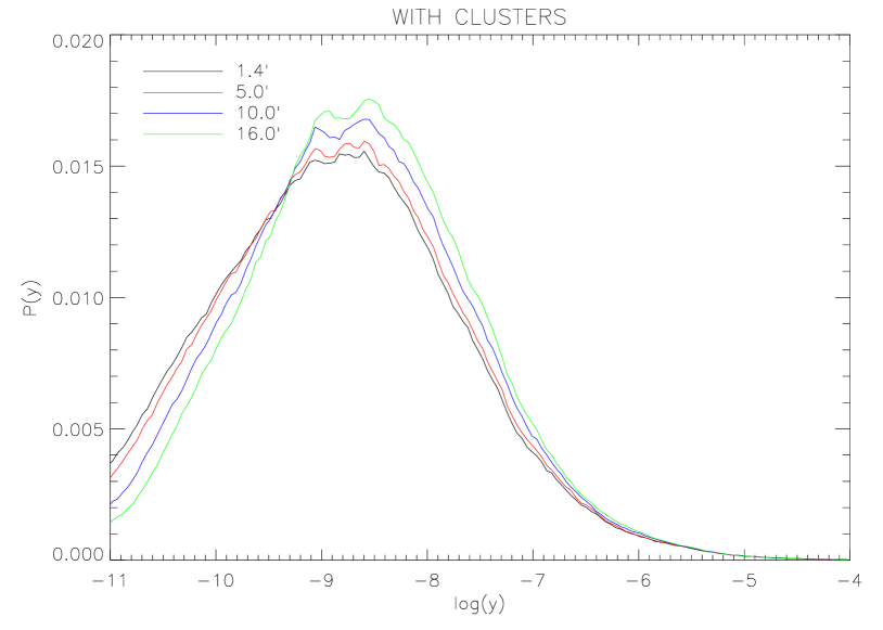
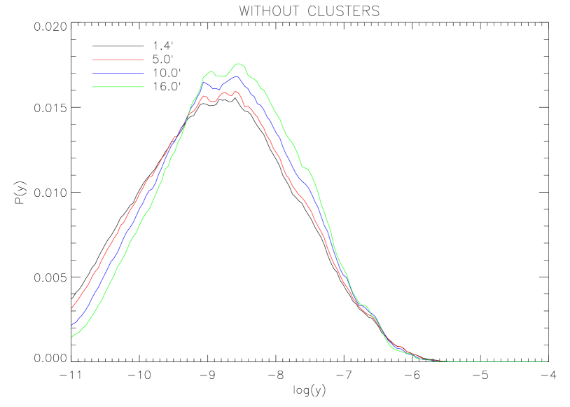
Figure 4: Averaged probability distribution for tSZ ($y$ parameter). These distributions are generated averaging over the nine subvolumes with clusters (top panel) and without clusters (bottom panel). The different colours correspond to the different resolutions used, as described in the legend. We can see that after the cluster subtraction, the upper tail of the distribution is significantly reduced.

Rotations of the tSZ maps.

We have carried out a statistical study to characterize the dependence of the tSZ signal on the different orientations of the observer with respect to the supercluster. Our aim is to quantify how random alignments of gas filaments along the line of sight affect the 1-PDF $y$-distributions. The top panel in Fig. 5 shows the nine 1-PDF curves after averaging over the 300 rotations in each case, while the bottom panel shows the 300 curves for a single subvolume. Note that when studying the upper tail of the 1-PDF for a single subvolume (bottom panel), the dispersion introduced by the rotations is very small, suggesting that the (few) objects which are producing those signals are probably very close to spherical. In other words, this high-$y$ tail is dominated by the contribution of clusters below the subtraction limit, or by galaxy groups. A very small number of possible orientations have yielded maximum values of the Comptonization parameter compatible at the 1 sigma level with the $y$-signal measured in the CrB-SC. We come back to this point in §5.

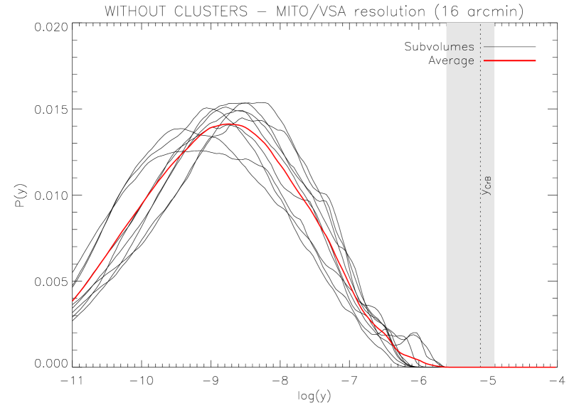
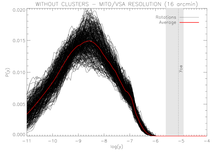
Figure 5: Top: Averaged (over the 301 rotations) one-point probability distribution functions of the $y$-maps for the nine independent subvolumes after cluster subtraction. The red line corresponds to the average of the nine curves. Bottom: 1-PDFs for the 301 maps obtained by rotations of a single subvolume. Again, the red line corresponds to the average of all black lines.

Relative contribution of the WHIM to the total tSZ signal.

We have also performed a detailed study of the separate contributions to the total tSZ effect from the different physical gas components: galaxy clusters, galaxy groups and WHIM. The different 1-PDF’s associated with each case are shown in Fig. 6, now only for the angular resolution of MITO/VSA (16’). As expected from the densities and temperatures of the different gas phases, galaxy clusters are responsible of the high-$y$ tail of the 1-PDF distribution, while groups and the WHIM have relevant contributions at the lowest $y$-values.

When comparing with the $y$-value measured in CrB-SC, these simulations show that only compact objects (most probably galaxy clusters, although we cannot completely discard groups of galaxies) are the only component that might build up a sufficiently large tSZ signal. Based on the probablility distributions obtained in our simulations, the WHIM is not a likely cause of the $y$-signal detected in the CrB-SC, as its probability distribution reaches the zero level at $y$ values much smaller than those of CrB. We will investigate this issue further in §5.

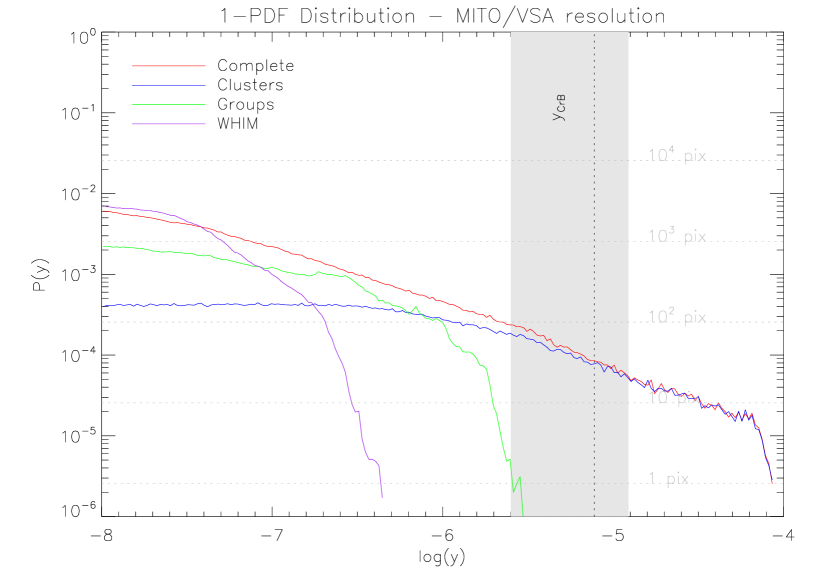
Figure 6: Averaged $y$ parameter probability distribution for the nine subvolumes. The different colours correspond to the different components found in the maps: all the objects, only clusters, only groups and only WHIM. The resolution of the maps used to compute these distributions is $16^{\prime}$, the MITO/VSA resolution. The shaded area corresponds to the $1\sigma$ interval of the observations in the CrB-SC and the horizontal dashed lines show the number of pixels that matches a given probability, showing that the WHIM fails to build up enough tSZ signal to be responsible for the spot observed in CrB-SC.

4.2.2 kSZ

Figure 7 shows the 1-PDF for the $b$ maps obtained from the nine sub-volumes, at the same angular resolutions as in Figure 4. These distributions show that only clusters contribute to the high kSZ effect tails, as one would in principle expect given their typical bulk velocities. Considering the rotations of the kSZ maps does not increases the maximum kSZ signals which are detected in the maps.

Figure 7: Same as Fig. 4, but for the $b$ parameter maps (kSZ component).

Finally, we have also studied the relative contribution of the kSZ component to the total SZ signal. As we can see in Fig. 8, the probability distribution of the temperature decrement seems almost unaffected when considering both tSZ and kSZ for all components except for the WHIM, in which case the probability distribution is slightly broadened with respect to the distribution considering tSZ only. This matches the expected result, as kSZ is only relevant to the total temperature decrement in regions with low temperatures, so neither clusters nor groups were expected to have a significant kSZ effect.

In any case, when considering the overall contribution of the different phases, it seems that the inclusion of a kSZ component cannot help in increasing the total SZ signal to the $-230$ $\mu$K observed with the VSA in the CrB-H spot. As a reference, Fig. 8 shows as a shaded region the one sigma confidence interval measured by MITO/VSA ($\Delta T_{\rm CrB}^{tSZ}\equiv-2y_{\rm CrB}$), and which accounts for 25% of the total observed decrement.

Figure 8: Probability distribution of the temperature decrements averaged over the nine different subvolumes and using MITO/VSA resolution $16^{\prime}$. Each colour shows a different component of the map, as given in the legend; solid lines represent only the contribution to the temperature decrement of the tSZ effect while dotted lines represent the total temperature decrement (considering both tSZ and kSZ). The shaded area corresponds to the $1\sigma$ interval of the observations carried out in the CrB-SC. The horizontal dashed lines indicate the equivalence between 1-PDF probability and the number of pixels in the maps.

5 The case of Corona Borealis

In the previous section, all the statistical analyses were focused on the description of global properties of the SZ signals associated with supercluster regions. We now restrict ourselves to the particular case of the detection of a significant negative feature in the Corona Borealis supercluster (CrB-SC) with the combined MITO/VSA experiments. The goal is twofold: on the one hand, we want to probe if the MNU simulations are able to explain the detected tSZ signal by MITO/VSA in terms of gas associated with the supercluster. On the other hand, we want to explore if the kSZ signal associated with the supercluster can be a plausible explanation for the rest of the observed decrement in the VSA map (a signal of the order of $-230$ $\mu$K). As pointed out above, even when we remove the observed tSZ component from the total VSA decrement, the remaining signal (roughly 75% of the total) is still difficult to reconcile with a primordial Gaussian CMB spot.

Given that the details of the sky coverage may introduce biases in the results, throughout this section we restrict our analyses to a sky coverage equivalent to the original VSA survey in which the cold spot was discovered, i.e. $\sim 24$ deg² (see Genova-Santos et al., 2005, for details). In practice, this means that all our analyses in each of the synthetic maps are restricted to a circle with an equivalent area of $24$ deg², centred on the central pixel of each map.

As shown in the previous section, the overall analysis in all the maps showed that the WHIM cannot provide a high enough tSZ signal to be the sole cause of the $y$-signal observed in the CrB-SC. When we include the contribution of groups of galaxies and small galaxy clusters (below the mass threshold for extraction), we cannot rule out completely the possibility that we might indeed be facing the cause of the observed $y$-signal. On the other hand, when considering the kSZ contribution, the total decrement that can be produced in this case is still far from the observed cold spot in the VSA map ($-230$ $\mu$K).

In order to quantify how likely groups and small clusters could yield tSZ signals in the confidence interval of the observations, and how large the contribution of the kSZ component to the total signal is, we have analysed the maximum amplitudes obtained in the simulated maps. The top panel of Table LABEL:table:max_maps shows these results for the case of the full maps (no cluster subtraction applied), while the bottom panel of the same table presents the case of the maps after the cluster subtraction (hence including groups and small clusters of galaxies). The three columns show the maximum values for the $y$ and $|b|$ parameters, and the largest temperature decrement in the Rayleigh–Jeans regime, computed as $\Delta T_{\rm RJ}\equiv(-2y+b)T_{0}$. The values in Table LABEL:table:max_maps are in good agreement with the typical peak amplitudes expected for the galaxy clusters in CrB, based on their X-ray luminosity (see the estimated values in Genova-Santos et al. (2005), based on the scaling relation between X-ray luminosity and tSZ peak temperature by Hernández-Monteagudo & Rubiño-Martín (2004)).

The values from the bottom panel of Table LABEL:table:max_maps are significantly smaller than those from the original maps, and we find that none of the subvolumes has maximum values within the $\pm 1\sigma$ range of the $y$-value observed in the CrB supercluster. If we consider a wider range, we find four subvolumes within the $\pm 1.3\sigma$ region of the $y$-signal, and all of them lie within the $\pm 1.36\sigma$ interval around the Comptonization parameter found in the CrB-SC observations.

That table also incorporates the maximum amplitudes (in absolute values) which are detected in the kSZ maps. While in the maps with clusters $y$ is about one order of magnitude larger than $b$, in the maps without clusters, both components of the SZE are comparable in amplitude, thus producing a larger temperature decrement in those cases in which the kSZ component contributes with a negative sign (i.e. a clump moving away from the observer). In any case, the addition of the kSZ cannot provide a significant contribution to the total temperature decrement observed by the VSA ($-230$ $\mu$K).

Table 4: Extreme values of SZ effect in the maps using MITO/VSA resolution. The top panel shows the results for the maps with clusters while the bottom panel corresponds to the cluster subtracted maps. Temperature values in the last column are obtained for the Rayleigh–Jeans region, in which we have $\Delta T_{\rm RJ}\equiv(-2y+b)T_{0}$.

	Maps with clusters
Subvol. #	$\max(y)$	$\max(|b|)$	$\Delta T_{\rm RJ}$
	$[10^{-6}]$	$[10^{-6}]$	$[\mu K]$
001	$67.4$	$2.90$	$-372.60$
002	$44.8$	$2.40$	$-244.91$
003	$82.0$	$7.64$	$-426.56$
004	$40.7$	$5.77$	$-207.81$
005	$16.4$	$2.09$	$-86.86$
006	$77.2$	$3.13$	$-418.34$
007	$87.7$	$6.48$	$-464.30$
008	$71.3$	$2.94$	$-394.63$
009	$30.9$	$6.62$	$-182.62$
	Maps with clusters subtracted
Subvol. #	$\max(y)$	$\max(|b|)$	$\Delta T_{\rm RJ}$
	$[10^{-6}]$	$[10^{-6}]$	$[\mu K]$
001	$1.05$	$1.31$	$-7.03$
002	$0.631$	$1.34$	$-5.64$
003	$0.613$	$0.995$	$-4.18$
004	$0.682$	$2.24$	$-2.30$
005	$0.886$	$1.21$	$-8.11$
006	$2.17$	$1.35$	$-11.60$
007	$0.618$	$0.497$	$-2.50$
008	$2.01$	$0.489$	$-11.44$
009	$0.691$	$0.763$	$-4.37$

5.1 Rotations

Here we also investigate how random alignments of matter along the line of sight might affect the maximum detectable SZ signal. The maximum values of tSZ, kSZ and total temperature decrement in the Rayleigh–Jeans regime, considering all 301 maps for each subvolume are summarized in the top section of Table LABEL:table:summary_rots. We also include the ranges of variation of these quantities (i.e. the difference between the highest and the lowest maximum signal found in any of the rotations), and the number of rotations in which the maps show maximum values of the Comptonization parameter compatible at the 1 sigma and 1.3 sigma levels with the observed $y$-signal in the CrB-SC. Note that when looking at the total temperature decrement we never obtain a value as high as the $-230$ $\mu$K observed for the full decrement by the VSA. Therefore, for the rest of this subsection we focus our attention on the tSZ component.

The full set of rotated $y$-maps also allows us to compute a crude estimate of the probability distribution function for the expected maximum values of the $y$ parameter at this resolution (MITO/VSA) and sky coverage ($24$ deg²), which is shown in Figure 9. Although the features in this curve are dominated by the fact that there are only 9 fully independent sub-volumes in the computation, this figure summarizes in a single plot the full range of $y$-values presented in Table LABEL:table:summary_rots.

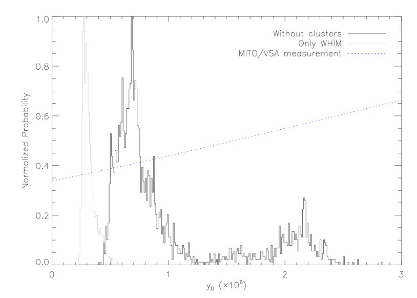
Figure 9: Top: Normalized probability distributions of the maximum values of the $y$ parameter. Black solid line shows this distribution for the maps without clusters (considering all 2709 maps; 301 maps per each subvolume), gray solid line shows the distribution for the maps that only include WHIM. Finally, the dotted line shows the posterior distribution of the SZ observations of the spot obtained in CrB with MITO/VSA. All distributions have been normalized to unity at their peak. Bottom: A zoom of the above plot around the region $[0,3\times 10^{-6}]$ in comptonization parameter.

The first conclusion is that even when selecting a “privileged” orientation of the supercluster with respect to the observer, the expected tSZ signals are still far from the MITO/VSA measurement obtained in CrB. Less than 0.3% of the rotations show values compatible at 1 sigma with the observations. Moreover, the range of variation of the maximum signals is very small (of the order of $50\%$ of the maximum signal), suggesting that the source of the high tSZ signals are compact and nearly spherical objects (most likely groups or small clusters of galaxies).

We again emphasize that these rotations only show the effect of the alignment of matter that belongs to the supercluster. Hence, the ranges of variation shown in table LABEL:table:summary_rots for each subvolume are only due to gas within $50~{}{\rm h}^{-1}~{}{\rm Mpc}$, either in groups of galaxies or in a diffuse phase.

Although the previous results firmly suggest that a $y$-signal like the one observed is unlikely caused exclusively by WHIM in the supercluster, we have again subjected the WHIM-only subvolumes to random rotations in order to verify this statement. A summary of the results is shown in the bottom part of Table LABEL:table:summary_rots, where we can see that the maximum tSZ effect caused by WHIM is $y\leq 5.6\times 10^{-7}$, hence, one order of magnitude smaller than the observations in the CrB-SC. The total temperature decrement also falls far from the observed value, always $\Delta T>-7.3$ $\mu$K, which is around 14 times smaller than $y_{\rm CrB}$. None of the randomly rotated WHIM maps yield SZ signals within the $1\sigma$ interval of the observations. Moreover, this contribution to the total tSZ signal would be masked by the contribution to the tSZ line of sight integral by the background of the region, which would be of the order of $<y>\approx 2\times 10^{-6}$ (see e.g. Springel et al., 2001; Roncarelli et al., 2007).

Hence, the second conclusion is that according to these simulations, the WHIM is not a likely cause of the spot, even at “privileged orientations“, where matter is aligned with the observer.

However, these conclusions do not take into account that the observations yielded a very broad posterior distribution, as seen in Fig. 9. Hence, we need to use a probability estimator that weights the probability distribution for the maximum values ($y_{\max}$) that we obtain in the simulation with this broad distribution. This probability is defined as follows:

$$P=\int_{0}^{\infty}\Big{(}\int_{y}^{\infty}P_{\rm s}(y_{\max})dy_{\max}\Big{)}P_{\rm obs}(y)dy$$ (6)

where $P_{\rm s}$ stands for the probability distribution for the $y_{\max}$ values in superclusters in the simulations and $P_{\rm obs}$ is the observed probability distribution for the spot. For this computation, we use the curves plotted in Fig. 9 (properly normalized to get a unity integral) as an estimate for $P_{\rm s}$, while $P_{\rm obs}$ is assumed to have a Gaussian shape with a sigma of $5.3\times 10^{-6}$, taken from the MITO/VSA observations. The integration of Eq. 6 gives a probability of $P=3.2\%$ for the maps without clusters (which still include groups) and a probability of $P=0.9\%$ for the maps that only include WHIM. Hence, supporting our conclusion that neither groups of galaxies, nor WHIM are likely explanations for the tSZ component of the spot.

Table 5: Orientation effects on the extreme values of the SZ effect, using the resolution of MITO/VSA in the maps. The top panel shows the results for cluster-subtracted maps (and hence includes the contribution of both the WHIM and small groups of galaxies). The bottom panel shows the results for the maps only considering the WHIM contribution. The columns show: (1) subvolume identification number; (2) maximum value of the $y$ parameter considering every map of the given subvolume, in units of $10^{-6}$; (3) minimum value of $y_{\rm max}$ obtained after rotations, in units of $10^{-6}$; (4) maximum of the absolute value of the $b$ parameter considering every map of the given subvolume, in units of $10^{-6}$; (5) minimum value of $|b|_{\rm max}$ obtained after rotations, in units of $10^{-6}$ (6) largest temperature decrement $\Delta T_{\rm min}$, expressed in $\mu K$ in the Rayleigh-Jeans regime, considering every map of the given subvolume. N.B. Temperature decrements are negative quantities, hence shown here are the minimum values obtained; (7) minimum temperature decrement in the Rayleigh-Jeans regime obtained after rotations, expressed in $\mu K$; (8) number of independent maps that yield maximum values of the $y$ parameter in the $\pm$1sigma range of CrB. (9) number of independent maps that yield maximum values of the $y$ parameter in the $\pm$1.3sigma range of CrB.

Maps with clusters subtracted (Only galaxy groups and WHIM)
Subvol.	$\max(y_{\rm max})$	$\min(y_{\rm max})$	$\max(|b|_{\rm max})$	$\min(|b|_{\rm max})$	$\min(\Delta T_{\rm min})$	$\max(\Delta T_{\rm min})$	$N_{\pm 1\sigma}$	$N_{\pm 1.3\sigma}$
	$[10^{-6}]$	$[10^{-6}]$	$[10^{-6}]$	$[10^{-6}]$	$[\mu K]$	$[\mu K]$
001	$1.39$	$0.77$	$1.80$	$0.68$	$-11.05$	$-5.64$	$0$	$193$
002	$1.30$	$0.42$	$2.08$	$0.83$	$-8.83$	$-3.62$	$0$	$19$
003	$1.08$	$0.54$	$1.48$	$0.91$	$-6.23$	$-3.22$	$0$	$7$
004	$1.04$	$0.58$	$2.65$	$1.46$	$-3.80$	$-1.56$	$0$	$19$
005	$1.07$	$0.49$	$1.60$	$0.91$	$-10.22$	$-5.44$	$0$	$8$
006	$2.62$	$1.25$	$1.35$	$0.42$	$-14.63$	$-6.84$	$5$	$301$
007	$1.01$	$0.44$	$1.89$	$0.44$	$-5.00$	$-1.76$	$0$	$18$
008	$2.84$	$1.57$	$1.03$	$0.40$	$-17.22$	$-8.94$	$3$	$301$
009	$1.05$	$0.60$	$2.57$	$0.62$	$-12.72$	$-4.17$	$0$	$4$
Only WHIM
Subvol.	$\max(y_{\rm max})$	$\min(y_{\rm max})$	$\max(|b|_{\rm max})$	$\min(|b|_{\rm max})$	$\min(\Delta T_{\rm min})$	$\max(\Delta T_{\rm min})$	$N_{\pm 1\sigma}$	$N_{\pm 1.3\sigma}$
	$[10^{-6}]$	$[10^{-6}]$	$[10^{-6}]$	$[10^{-6}]$	$[\mu K]$	$[\mu K]$
001	$0.51$	$0.22$	$0.91$	$0.36$	$-3.91$	$-1.51$	$0$	$0$
002	$0.53$	$0.19$	$1.57$	$0.75$	$-6.25$	$-3.11$	$0$	$0$
003	$0.50$	$0.25$	$1.49$	$0.64$	$-4.55$	$-2.01$	$0$	$0$
004	$0.55$	$0.21$	$2.25$	$1.07$	$-2.39$	$-0.93$	$0$	$0$
005	$0.49$	$0.24$	$1.10$	$0.49$	$-4.84$	$-3.01$	$0$	$0$
006	$0.42$	$0.15$	$1.15$	$0.46$	$-4.05$	$-0.82$	$0$	$0$
007	$0.36$	$0.15$	$1.19$	$0.31$	$-3.28$	$-1.01$	$0$	$0$
008	$0.46$	$0.21$	$0.82$	$0.29$	$-3.49$	$-1.38$	$0$	$0$
009	$0.48$	$0.10$	$1.73$	$0.43$	$-7.32$	$-1.61$	$0$	$0$

6 Observability of diffuse SZ signals from superclusters with Planck

Although this was not the main motivation of this paper, the same set of MNU simulations can be used to predict the expected level of SZ signals in superclusters of galaxies that could be detectable with the Planck satellite. To this end, we have convolved all the maps to a common (nominal) resolution of $5$ arcmin and we present here a brief discussion of this topic by repeating the same kind of analysis that was done in previous section.

We concentrate here on “diffuse” SZ signals associated with superclusters, where for the purposes of this paper “diffuse” means “all gas phases which contribute to the SZ signal but excluding all clusters with masses $M\geq 5\times 10^{13}$ $~{}{\rm h}^{-1}~{}{\rm M}_{\odot}$” (i.e. our maps with clusters subtracted). A detailed study of the contribution of unresolved galaxy clusters (i.e. clusters with fluxes below the detection threshold for Planck, but with masses greater than $5\times 10^{13}$ $~{}{\rm h}^{-1}~{}{\rm M}_{\odot}$) is beyond the scope of this paper.

Table LABEL:table:SZ_with_Planck shows the expected range of variation for the maximum SZ signals (both tSZ and kSZ) originating in superclusters of galaxies without considering the contribution of the clusters themselves. The top panel includes the contribution of groups of galaxies and diffuse gas while the bottom panel shows only the WHIM contribution. Taking into account the nominal sensitivities of the Planck satellite (e.g. 6 $\mu$K at 143 GHz with 7.1 arcmin beam, or 13 $\mu$K at 217 GHz with a 5 arcmin beam), direct detections of individual features due to groups+WHIM signals might be feasible provided that a good correction of the rest of the foreground components is achieved. However, a direct detection of an individual feature due to WHIM alone seems more difficult, although in principle it would be possible at the 2 or 3 sigma level.

Finally, and for illustrative purposes only, we make here a simple comparison with the extrapolated CrB-SC $y$-parameter value, which was measured using MITO/VSA. To this end, we consider two reference values, namely the peak of the $y$-parameter, and the minus one-sigma value, and we re-scale those two numbers by assuming that scale factor is the one for a point-like object. In this case, we obtain $8.0\times 10^{-5}$ and $2.6\times 10^{-5}$ for the central and minus one-sigma values, respectively. We note that those values are an order of magnitude larger than the maximum tSZ signals obtained in the maps without clusters. Hence, if we consider the Planck resolution, the numerical simulations are not able to explain tSZ signals as high as the one measured in CrB-SC (provided that the object producing it is point-like) in terms of hot gas in the supercluster which is not in clusters of galaxies. A more detailed study would require the modelling of the spot shape, which is beyond the scope of this article.

Table 6: Forecast of the maximum expected values for the diffuse SZ signals in supercluster of galaxies for Planck. For these computations, we adopt an angular resolution of 5 arcmin. For the meaning of the different columns, see Table LABEL:table:summary_rots for comparison.

Maps with clusters subtracted (Only galaxy groups and WHIM)
Subvol.	$\max(y_{\rm max})$	$\min(y_{\rm max})$	$\max(|b|_{\rm max})$	$\min(|b|_{\rm max})$	$\min(\Delta T_{\rm min})$	$\max(\Delta T_{\rm min})$
	$[10^{-6}]$	$[10^{-6}]$	$[10^{-6}]$	$[10^{-6}]$	$[\mu K]$	$[\mu K]$
001	$3.07$	$1.56$	$7.25$	$3.90$	$-36.50$	$-19.67$
002	$2.91$	$0.94$	$6.05$	$2.98$	$-26.48$	$-13.05$
003	$4.26$	$2.02$	$4.62$	$3.68$	$-19.52$	$-9.82$
004	$3.36$	$1.42$	$8.89$	$4.69$	$-13.85$	$-4.18$
005	$3.55$	$2.32$	$5.78$	$4.14$	$-34.73$	$-24.03$
006	$4.31$	$1.74$	$3.26$	$1.41$	$-23.17$	$-10.86$
007	$2.35$	$0.84$	$5.67$	$1.36$	$-15.47$	$-5.88$
008	$5.77$	$2.46$	$2.71$	$1.49$	$-30.84$	$-14.45$
009	$2.87$	$0.86$	$5.57$	$1.65$	$-25.22$	$-7.26$
Only WHIM
Subvol.	$\max(y_{\rm max})$	$\min(y_{\rm max})$	$\max(|b|_{\rm max})$	$\min(|b|_{\rm max})$	$\min(\Delta T_{\rm min})$	$\max(\Delta T_{\rm min})$
	$[10^{-6}]$	$[10^{-6}]$	$[10^{-6}]$	$[10^{-6}]$	$[\mu K]$	$[\mu K]$
001	$1.94$	$0.80$	$3.26$	$1.57$	$-14.77$	$-5.99$
002	$1.76$	$0.86$	$6.06$	$3.22$	$-25.99$	$-12.93$
003	$1.64$	$0.83$	$3.91$	$1.78$	$-16.20$	$-8.18$
004	$1.69$	$0.88$	$7.69$	$3.54$	$-8.37$	$-3.85$
005	$1.55$	$0.67$	$2.70$	$1.38$	$-12.47$	$-7.05$
006	$1.35$	$0.49$	$2.72$	$1.46$	$-11.14$	$-2.80$
007	$1.14$	$0.69$	$3.79$	$1.08$	$-9.32$	$-5.51$
008	$1.37$	$0.84$	$2.52$	$1.41$	$-10.88$	$-6.74$
009	$1.31$	$0.44$	$5.32$	$1.59$	$-18.85$	$-6.69$

7 Discussion and Conclusions

Based on the nine supercluster regions extracted from the MNU simulation, our main conclusion is that a Comptonization $y$-parameter as large as the one measured in CrB-SC by MITO/VSA is probably produced by galaxy clusters ($M\geq 5\times 10^{13}$ $~{}{\rm h}^{-1}~{}{\rm M}_{\odot}$). When excluding the tSZ component associated with galaxy clusters, the maximum $y$-values are typically of the order of $y\lesssim 2\times 10^{-6}$. Exceptionally, we do obtain orientations in which the maximum value is compatible at the lower end of the 1 sigma level (with a largest value of $y\sim 2.84\times 10^{-6}$). However, these “privileged” orientations represent less than 0.3% of all the cases. When we take into account the actual posterior distribution from the observations as described in equation 6, the probability of finding CrB-like features in the maps without clusters is $3.2\%$. Moreover, those values are comparable to (and in some cases smaller than) the expected contribution to the los SZ integral by background clusters (see e.g. Springel et al., 2001; Roncarelli et al., 2007). Hence, it seems more plausible that the $y$-signal observed in the CrB-SC is caused by a cluster of galaxies that does not belong to the supercluster, and that is located further along the line of sight, instead of the hypothesis that the spot is being produced by small clusters or galaxy groups associated to the supercluster.

On the other hand, and if our simulations provide a suitable description to the gas physics, the WHIM phase, defined as gas with $10^{5}K<T<10^{7}K$, cannot build up a tSZ signal compatible with the observations. If we take into account the posterior distribution from the observations, the probability of finding tSZ signals compatible with the observations (see eq. 6) is smaller than $1\%$. Hence, although we can not rule out a contribution of WHIM from the supercluster, it is unlikely the cause of the spot in CrB.

Including the kSZ component does not modify this conclusion. However, the simulations show that the kinematic component of the SZE plays an important role in building up the total temperature decrement in the maps with clusters removed. Whereas in clusters kSZ is about one order of magnitude lower than tSZ, when clusters are excluded from the analysis, both SZ components are comparable. This role is also noticeable in the temperature decrement probability distribution, showing that in order to study the SZ effect due to WHIM, kSZ should not be neglected. This idea seems to be supported by the work done by Atrio-Barandela et al. (2008), where it is shown that the kSZ effect originates in filaments of gas of certain characteristics could yield temperature decrements comparable to those of CrB. However, it should be noted that we have not been able to reproduce the temperature anisotropies they predict, considering galaxy groups plus WHIM in our simulations.

Our main conclusion might in principle depend on the cosmology. The MNU simulation has been obtained using a rather large normalization power spectrum to set up the initial conditions. Current WMAP5 results indicate smaller values for both $\sigma_{8}$ and $\Omega_{\rm m}$ than the ones we used in the simulation. This will translate into less evolved structures, where the abundance of massive clusters in the same volume is considerably suppressed as was shown in Yepes et al. (2007) from a set of different MareNostrum simulations with WMAP1 and WMAP3 cosmological parameters. This means that, attending only to the cosmology, the results shown in this paper constitute an upper limit to the probability of finding features like the CrB spot for the same cosmic volume sampled. We cannot neglect either the effect of cosmic variance: using a larger volume we would have been able to extend the sample of superclusters and thus improve the statistics in order to obtain a better probability function. However, according to the variance shown in the simulation, we do not expect significant changes in the results.

The other caveat concerns the modelling of the physics of baryons in clusters. MNU is a pure adiabatic gasdynamical simulation where radiative processes are not taken into account. The inclusion of radiative cooling, UV photoionization and star formation would change the properties of the gas inside clusters and the corresponding SZ effect. How large this change is not a simple answer since we are not yet able to perform large scale simulations of the size of the MareNostrum Universe but including also cooling and star formation effects. According to Cen & Ostriker (2006), the inclusion of these feedback effects does not significantly modify the fraction of baryons expected in the WHIM. However, feedback does slightly modify the differential mass fraction, heating the gas from the warm phase ($T\lesssim 10^{5}K$) into the WHIM phase, while the hot phase ($T\gtrsim 10^{7}K$) remains unchanged. Given that the greatest SZ effect from the WHIM originates in the phase with $T\sim 10^{7}K$ (e.g. Hernández-Monteagudo et al., 2006), our results seem fairly robust against feedback. Nonetheless, it should be further studied, especially since shocks could play a very important role in heating the gas in the CrB cluster and hence be the cause of the spot. Despite the lack of large scale simulations with feedback effects, one possibility for this study is to perform a re-simulation of a volume-limited sample of clusters in which considerably more physical processes are to be included. This will allow us to estimate the relative change in the determination of the SZ effect with respect to the adiabatic runs and estimate the effect of shocks. This is a future project.

All in all, and according to the description provided by the MNU gasdynamical simulations, we conclude that the observed thermal SZ component of the CrB H-spot most probably arises from one (or several) unknown galaxy cluster(s) along the line of sight, which in principle are not neccesarily associated with the CrB supercluster. In order to explore this idea further, we have started an observational programme to perform a detailed characterization of the properties of the galaxy populations along the line of sight of the CrB spot (see Padilla-Torres et al., 2009).

References

- Atrio-Barandela & Mücket (2006) Atrio-Barandela F., Mücket J. P., 2006, ApJ, 643, 1
- Atrio-Barandela et al. (2008) Atrio-Barandela F., Mücket J. P., Génova-Santos R., 2008, ApJL, 674, L61
- Battistelli et al. (2007) Battistelli E. S., De Petris M., Lamagna L., Watson R. A., Rebolo R., Génova-Santos R., Luzzi G., De Gregori S., Rubiño-Martin J. A., 2007, New Astronomy Review, 51, 374
- Battistelli et al. (2006) Battistelli E. S., De Petris M., Lamagna L., Watson R. A., Rebolo R., Melchiorri F., Génova-Santos R., et al., 2006, ApJ, 645, 826
- Birkinshaw (1999) Birkinshaw M., 1999, Phys.Rep., 310, 97
- Boughn (1999) Boughn S. P., 1999, ApJ, 526, 14
- Buote et al. (2009) Buote D. A., Zappacosta L., Fang T., Humphrey P. J., Gastaldello F., Tagliaferri G., 2009, ArXiv e-prints
- Burles et al. (2001) Burles S., Nollett K. M., Turner M. S., 2001, ApJL, 552, L1
- Carlstrom et al. (2000) Carlstrom J. E., Joy M. K., Grego L., Holder G. P., Holzapfel W. L., Mohr J. J., Patel S., Reese E. D., 2000, Physica Scripta Volume T, 85, 148
- Cen & Ostriker (1999) Cen R., Ostriker J. P., 1999, ApJ, 514, 1
- Cen & Ostriker (2006) Cen R., Ostriker J. P., 2006, ApJ, 650, 560
- Da Silva et al. (2000) Da Silva A. C., Barbosa D., Liddle A. R., Thomas P. A., 2000, MNRAS, 317, 37
- De Petris et al. (1999) De Petris M., Mainella G., Nerozzi A., de Bernardis P., Garavini G., Granata S., Guarini G., Masi S., Melchiorri B., Melchiorri F., Nobili S., Orlando A., Palummo L., Pisano G., Terracina A., 1999, New Astronomy Review, 43, 297
- Dolag et al. (2005) Dolag K., Hansen F. K., Roncarelli M., Moscardini L., 2005, MNRAS, 363, 29
- Einasto et al. (2001) Einasto M., Einasto J., Tago E., Müller V., Andernach H., 2001, AJ, 122, 2222
- Fukugita et al. (1998) Fukugita M., Hogan C. J., Peebles P. J. E., 1998, ApJ, 503, 518
- Génova-Santos et al. (2008) Génova-Santos R., Rubiño-Martín J. A., Rebolo R., Battye R. A., Blanco F., Davies R. D., Davis R. J., Franzen T., et al., 2008, MNRAS, 391, 1127
- Genova-Santos et al. (2005) Genova-Santos R., Rubiño-Martin J. A., Rebolo R., Cleary K., Davies R. D., Davis R. J., Dickinson C., Falcon N., Grainge K., et al., 2005, MNRAS, 363, 79
- Gill et al. (2004) Gill S. P. D., Knebe A., Gibson B. K., 2004, MNRAS, 351, 399
- Gottlöber & Yepes (2007) Gottlöber S., Yepes G., 2007, ApJ, 664, 117
- Gottlöber et al. (2006) Gottlöber S., Yepes G., Wagner C., Sevilla R., 2006, ArXiv Astrophysics e-prints
- Hallman et al. (2007) Hallman E. J., O’Shea B. W., Burns J. O., Norman M. L., Harkness R., Wagner R., 2007, ApJ, 671, 27
- Hallman et al. (2009) Hallman E. J., O’Shea B. W., Smith B. D., Burns J. O., Norman M. L., 2009, ArXiv e-prints
- Hansen et al. (2005) Hansen F. K., Branchini E., Mazzotta P., Cabella P., Dolag K., 2005, MNRAS, 361, 753
- Hernández-Monteagudo & Rubiño-Martín (2004) Hernández-Monteagudo C., Rubiño-Martín J. A., 2004, MNRAS, 347, 403
- Hernández-Monteagudo et al. (2006) Hernández-Monteagudo C., Trac H., Verde L., Jimenez R., 2006, ApJL, 652, L1
- Kitayama & Suto (1996) Kitayama T., Suto Y., 1996, ApJ, 469, 480
- Klypin et al. (1999) Klypin A., Gottlöber S., Kravtsov A. V., Khokhlov A. M., 1999, ApJ, 516, 530
- Knollmann & Knebe (2009) Knollmann S. R., Knebe A., 2009, ApJS, in press
- Nicastro et al. (2005) Nicastro F., Mathur S., Elvis M., Drake J., Fiore F., Fang T., Fruscione A., Krongold Y., Marshall H., Williams R., 2005, ApJ, 629, 700
- Nicastro et al. (2003) Nicastro F., Zezas A., Elvis M., Mathur S., Fiore F., Cecchi-Pestellini C., Burke D., Drake J., Casella P., 2003, Nature, 421, 719
- Padilla-Torres et al. (2009) Padilla-Torres C. P., Gutierrez C. M., Rebolo R., Genova-Santos R., Rubino-Martin J. A., 2009, ArXiv e-prints
- Persic et al. (1990) Persic M., Jahoda K., Rephaeli Y., Boldt E., Marshall F. E., Mushotzky R. F., Rawley G., 1990, ApJ, 364, 1
- Persic et al. (1988) Persic M., Rephaeli Y., Boldt E., 1988, ApJL, 327, L1
- The Planck Collaboration (2006) The Planck Collaboration 2006, arXiv:astro-ph/0604069, also available online444http://www.rssd.esa.int/index.php?project=Planck&page=pubdocs_top.
- Rauch et al. (1997) Rauch M., Miralda-Escude J., Sargent W. L. W., Barlow T. A., Weinberg D. H., Hernquist L., Katz N., Cen R., Ostriker J. P., 1997, ApJ, 489, 7
- Rebolo et al. (2004) Rebolo R., Battye R. A., Carreira P., Cleary K., Davies R. D., Davis R. J., Dickinson C., Genova-Santos R., et al., 2004, MNRAS, 353, 747
- Roncarelli et al. (2007) Roncarelli M., Moscardini L., Borgani S., Dolag K., 2007, MNRAS, 378, 1259
- Rubiño-Martín et al. (2006) Rubiño-Martín J. A., Aliaga A. M., Barreiro R. B., Battye R. A., Carreira P., Cleary K., Davies R. D., Davis R. J., Dickinson C., Génova-Santos R., et al., 2006, MNRAS, 369, 909
- Rubiño-Martín & Sunyaev (2003) Rubiño-Martín J. A., Sunyaev R. A., 2003, MNRAS, 344, 1155
- Savage et al. (1998) Savage B. D., Tripp T. M., Lu L., 1998, AJ, 115, 436
- Small et al. (1997) Small T. A., Sargent W. L. W., Hamilton D., 1997, ApJS, 111, 1
- Spergel et al. (2007) Spergel D. N., Bean R., Doré O., Nolta M. R., Bennett C. L., Dunkley J., Hinshaw G., Jarosik N., Komatsu E., Page L., Peiris H. V., Verde L., Halpern M., Hill R. S., Kogut A., Limon M., Meyer S. S., Odegard N., Tucker G. S., et al., 2007, ApJS, 170, 377
- Springel (2005) Springel V., 2005, MNRAS, 364, 1105
- Springel et al. (2001) Springel V., White M., Hernquist L., 2001, ApJ, 549, 681
- Springel et al. (2001) Springel V., Yoshida N., White S. D. M., 2001, New Astronomy, 6, 79
- Staniszewski et al. (2008) Staniszewski Z., Ade P. A. R., Aird K. A., Benson B. A., Bleem L. E., Carlstrom J. E., Chang C. L., Cho H. ., Crawford T. M., Crites A. T., de Haan T., Dobbs M. A., Halverson N. W., Holder G. P., Holzapfel W. L., Hrubes J. D., Joy M., Keisler R., et al., 2008, ArXiv e-prints
- Sunyaev & Zeldovich (1972) Sunyaev R. A., Zeldovich Y. B., 1972, Comments on Astrophysics and Space Physics, 4, 173
- Watson et al. (2003) Watson R. A., Carreira P., Cleary K., Davies R. D., Davis R. J., Dickinson C., Grainge K., Gutiérrez C. M., Hobson M. P., Jones M. E., Kneissl R., Lasenby A., Maisinger K., Pooley G. G., Rebolo R., Rubiño-Martin J. A., et al., 2003, MNRAS, 341, 1057
- Yepes et al. (2007) Yepes G., Sevilla R., Gottlöber S., Silk J., 2007, ApJL, 666, L61