On the smooth cross-over transition from the $\Delta$-string to the Y-string three-quark potential

Abstract

We comment on the assertion made by Caselle et al. Caselle:2005sf that the confining (string) potential for three quarks “makes a smooth cross-over transition from the $\Delta$-string to the Y-string configuration at interquark distances of around 0.8 fm”. We study the functional dependence of the three-quark confining potentials due to a Y-string, and the $\Delta$ string and show that they have different symmetries, which lead to different constants of the motion (i.e. they belong to different “universality classes” in the parlance of the theory of phase transitions). This means that there is no “smooth cross-over” between the two, when their string tensions are identical, except at the vanishing hyper-radius. We also comment on a certain two-body potential approximation to the Y-string potential.

I Introduction

The so-called Y-junction string three-quark potential, defined by

$$V_{Y}=\sigma\min_{\bf x_{0}}\;\sum_{i=1}^{3}|{\bf x_{i}}-{\bf x_{0}}|.$$ (1)

has long been advertised artr75 ; dosc76 as the natural approximation to the flux tube confinement mechanism, that is allegedly active in QCD. Lattice investigations, Refs. taka01 ; Alex01 , however, contradict each other in their attempts to distinguish between the Y-string, Fig. 1, and the $\Delta$-string potential, see Fig. 2,

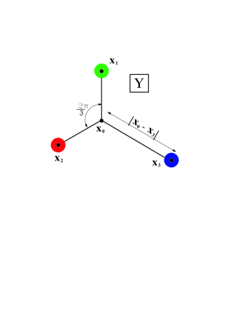
Figure 1: Three-quark Y-junction string potential.

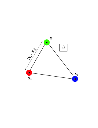
Figure 2: Three-quark $\Delta$-shape string potential.

$$V_{\Delta}=\sigma\sum_{i<j=1}^{3}|{\bf x}_{i}-{\bf x}_{j}|,$$ (2)

which, in turn, is indistinguishable from the sum of three linear two-body potentials. One may therefore view the present lattice results as inconclusive and await the next generation of lattice calculations. Another point of view held among some lattice QCD practitioners deForcrand:2005vv is that there should be a smooth cross-over from the $\Delta$ to the Y-potential at interquark distances of around 0.8 fm. This opinion is based on certain similarities between the Potts model and lattice QCD which were made more precise in Ref. Caselle:2005sf . It was not stated in Ref. Caselle:2005sf , however, how exactly this cross-over should be implemented, nor what they meant by “interquark distances”.

In the course of our studies of the (difference between the) Y-string and the $\Delta$-string potentials dss09 , we have taken this assertion at face value and tried to devise a “smooth cross-over”, i.e. to make a smooth interpolation between these two potentials, that is as simple as possible. What we found is simple enough to state: there can be no smooth cross-over interpolation between these two potentials; there must be always a discontinuity in some variable(s). This fact may perhaps even be simply understood on the basis of the different topologies of the two configurations, see the discussion below, but the proof which we show (in some detail) is complicated by the (technical) requirements of the $S_{3}$ permutation symmetry.

We shall address the above questions one after another and for this reason we divide the paper in four sections. In Sect. II, we define the potentials that we use, in the second Sect. III, we show an analytic proof of incompatibility of $\Delta$ and Y-strings, and finally the third Sect. IV, addresses approximations to the string potentials that can be used to extract results from the lattice or to be used in the constituent quark model. The final Section V contains a summary of our results and the discussion.

II Three-body potentials

Any reasonable static, spin-independent three-body potential must be: 1) translation-invariant, which means that it must depend only on the two linearly independent relative coordinates, which we call $({\bm{\rho}},{\bm{\lambda}})$, but not on the center-of-mass coordinate; 2) rotation-invariant, which means that it may depend only on the three scalar products of the relative coordinates ${\bm{\rho}}^{2},{\bm{\lambda}}^{2},({\bm{\rho}}\cdot{\bm{\lambda}})$; and 3) permutation-invariant, which means that it may depend only on certain combinations, yet to be determined, of the above three scalar products of the relative coordinates.

We shall show that there are (precisely) three independent permutation symmetric functions/variables of the relative coordinates, that are related to simple geometrical/physical properties (the moment of inertia, the area, and the perimeter of the triangle) which clearly distinguishes them, and that the potential’s dependence on any one of them in particular carries dynamical consequences.

Then we show that the (central, or three-body part of, for precise definition see Sect. II.1.2 below) Y-string potential depends on only two (the moment of inertia and the area of the triangle, but not on the perimeter) of these three variables in most geometrical configurations; whereas the $\Delta$-string potential depends only on the perimeter.

II.1 Derivation of the $\Delta$- and Y-string potentials

II.1.1 Derivation of the $\Delta$-string potentials

The $\Delta$-string potential

$$V_{\Delta}=\sigma\sum_{i<j=1}^{3}|{\bf x}_{i}-{\bf x}_{j}|=2\sigma s,$$ (3)

is proportional to the perimeter of the triangle $2s=(a+b+c)$, where $a=AB,b=BC,c=CA$ are the three sides of the triangle and A,B,C are a positions of the quarks. When written in this form, the potential is manifestly translation-, rotation- and permutation invariant.

II.1.2 Derivation of the Y-string potential

Three strings (“flux tubes”) merge at the point $\bf x_{0}$, which is chosen such that the sum of their lengths $l_{3q}=l_{Y}$ is minimized

$$l_{\rm Y}=\min_{\bf x_{0}}\;\sum_{i=1}^{3}|{\bf x_{i}}-{\bf x_{0}}|.$$ (4)

If all the angles in the triangle are less than 120^∘, then the equilibrium Y-junction position is the so-called Toricelli (or Fermat, or Steiner) point of classical geometry, $I={\bf x}_{0}$ in Fig. 1 that has the property that the straight lines emanating from the junction point ${\bf x}_{0}$ and leading to the quarks (“strings”) all form an angle $2\pi/3$ at (see Fig. 1). The corresponding “three-string length $l_{Y}$ is

$$l_{Y} = \sqrt{\frac{1}{2}(AB^{2}+BC^{2}+CA^{2})+2\sqrt{3}{\rm Area\triangle ABC}}\quad\text{if}\quad\measuredangle\widehat{A},\measuredangle\widehat{B},\measuredangle\widehat{C}\leq 120^{\circ},\$$ (5)

where $a=AB,b=BC,c=CA$ are the three sides of the triangle. Here one can see that the “three-string” potential Eq. (5) depends on the “harmonic oscillator” variable $(a^{2}+b^{2}+c^{2})$, which is permutation symmetric and proportional to the moment of inertia (divided by the quark mass) of this triangle , and on the triangle area

$${\rm Area\triangle ABC} = \frac{1}{4}\sqrt{(AB+BC+CA)(-AB+BC+CA)(AB-BC+CA)(AB+BC-CA)}$$ (6)

$$= \triangle(a,b,c)=\frac{1}{4}\sqrt{2(a^{2}b^{2}+b^{2}c^{2}+b^{2}c^{2})-a^{4}-b^{4}-c^{4}},$$

which is also permutation symmetric.

This form of the Y-string potential, when expressed in terms of triangle sides $(a,b,c)$ only, exhibits its permutation symmetry $S_{3}$, but hides the hidden/implicit angular dependence of the potential, and potential interdependencies on other permutation symmetric variables: The triangle area can be written using Heron’s formula

$${\rm Area\triangle ABC} = \sqrt{s(s-a)(s-b)(s-c)},$$ (7)

as a function of the triangle’s semi-perimeter $s=\frac{1}{2}(a+b+c)$ and the three sides $a,b,c$.

It should be intuitively clear, however, that the perimeter and the area of the triangle are two independent properties of the triangle. Moreover, all three variables have non-zero dimensionality, which seems to imply that there are three different measures of “intequark distances”. The task now becomes to find the most suitable independent coordinates/variables for an interpolation.

If one of the angles within the triangle equals or exceeds the value $2\pi/3=120^{\circ}$, however, the corresponding vertex of the triangle is the junction point (although the Toricelli point can be constructed in that case, as well, but generally lies outside of the triangle and need not coincide with the vertex) and the minimal two-string length is

$$l_{V} = (a+c)\quad\text{if}\quad\alpha=\measuredangle\widehat{A}\geq 120^{\circ},\quad\cos\alpha=\frac{1}{2ac}(a^{2}+c^{2}-b^{2})\leq-\frac{1}{2}$$ (8)

$$= (a+b)\quad\text{if}\quad\beta=\measuredangle\widehat{B}\geq 120^{\circ},\quad\cos\beta=\frac{1}{2ab}(a^{2}+b^{2}-c^{2})\leq-\frac{1}{2}$$ (9)

$$= (b+c)\quad\text{if}\quad\gamma=\measuredangle\widehat{C}\geq 120^{\circ},\quad\cos\gamma=\frac{1}{2bc}(b^{2}+c^{2}-a^{2})\leq-\frac{1}{2}$$ (11)

$$\quad\text{where $a=AB,b=BC,c=CA$}.$$

Each one of these three expressions explicitly violates the permutation symmetry (because of the “missing piece of string”), but taken in totality they maintain it, in the sense that no one vertex is different from the others when its angle exceeds $2\pi/3=120^{\circ}$.

II.2 String potentials in terms of relative coordinates

The three sides of a triangle are not be the most useful coordinates for practical calculations, however. Below, we shall express these potentials in terms of conventional three-body Jacobi relative coordinates ${\bm{\rho}},{\bm{\lambda}}$

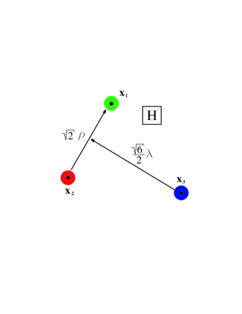
Figure 3: Two three-body Jacobi coordinates $\rho,\lambda$ that define the “hyper-radial” string length $\sqrt{|{\bm{\rho}}|^{2}+|{\bm{\lambda}}|^{2}}$.

$${\bm{\rho}}_{12} = \frac{1}{\sqrt{2}}({\bf x_{1}}-{\bf x_{2}}),$$ (12)

$${\bm{\lambda}}_{12} = \frac{1}{\sqrt{6}}({\bf x_{1}}+{\bf x_{2}}-2{\bf x_{3}}),$$ (13)

$${\bf x_{\rm CM}} = \frac{1}{3}({\bf x_{1}}+{\bf x_{2}}+{\bf x_{3}}),\$$ (14)

which obscures the permutation symmetry, however (see Sect. III.0.1). From now on, we always specialize to the pair (12) and drop the 12 index everywhere, so that the Jacobi coordinates in our problem will be denoted by ${\bm{\rho}}$ (instead of ${\bm{\rho}}_{12}$) and ${\bm{\lambda}}$ (instead of ${\bm{\lambda}}_{12}$).

II.2.1 String potentials in terms of hyper-spherical coordinates

We receive help here in the form of hyper-spherical coordinates: instead of the moduli $\rho$ and $\lambda$ of the two Jacobi vectors ${\bm{\lambda}},{\bm{\rho}}$, shown in Fig. 3, the hyper-spherical coordinates introduce the hyper-radius, which is permutation symmetric:

$$R=\sqrt{\rho^{2}+\lambda^{2}},$$ (15)

as the only variable with dimension of length, the hyper-angle $\chi$ through the polar transformation

$$\rho=R\sin\chi,\quad\lambda=R\cos\chi\quad\text{with}\quad 0\leq\chi\leq\pi/2.$$ (16)

and the (physical) angle $\theta$ between ${\bm{\lambda}}$ and ${\bm{\rho}}$: $\cos\theta={\bm{\lambda}}\cdot{\bm{\rho}}/(\rho\lambda)$. The boundary in the $\chi$ vs. $\theta$ plane between the regions in which the two- and the three-string potentials are valid is determined by Eqs. (17). There are three such boundaries, determined by the three (in)equalities, that merge continuously one into another at two “contact points” and one line, see Fig. 4.

$$\cot\chi_{1}(\theta) = \frac{-1}{{\sqrt{3}}\,\cos\theta+\sin\theta},$$

$$\cot\chi_{2}(\theta) = \frac{1}{{\sqrt{3}}\,\cos\theta-\sin\theta},$$

$$\cot\chi_{3}(\theta) = \frac{1}{3}{\sqrt{5-2\,{\cos}^{2}\theta-2\,|\sin\theta|\,{\sqrt{4-\cos^{2}\theta}}}}.\$$ (17)

Figure 4: The boundary in the $\chi$ vs. $\theta$ plane, between the regions in which the two- and the three-string potentials are appropriate, see Eqs. (17). The three-string potential holds in the central region, whereas the two-string potential holds in the “corners” of this parallelogram.

The two hyper-angles ($\chi$, $\theta$) describe the shape of the triangle, so the ($z=\cos 2\chi$, $x=\cos\theta$) plane (square) may be termed the “shape-space”. Manifestly, for each angle $\theta$ there is another configuration with angle $\pi-\theta$ that describes a “similar” triangle geometry that is a mirror image of the other. For this reason any three-body potential defined by geometric variables must be symmetric under reflections across the $\theta=\pi/2$ axis. In Figs. 5, 6 we show contour plots of the Y-string and the $\Delta$-string potentials, respectively, in the “shape space” plane, i.e as functions of $z=\cos 2\chi$ (vertical axis) and $x=\cos\theta$ (horizontal axis), where this symmetry is plain to behold.

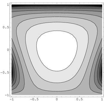
Figure 5: Contour plot of the $\Delta$-string potential as a function of the cosines of the two hyper-angles $z=\cos 2\chi$ (vertical axis) and $x=\cos\theta$ (horizontal axis) at any fixed value of the hyper-radius $R$. The darker regions indicate a smaller value of the potential. The reflection symmetry about the x=0 axis should be visible to the naked eye.

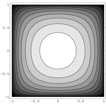
Figure 6: Contour plot of the Y-string potential as a function of the cosines of the two hyper-angles $z=\cos 2\chi$ (vertical axis) and $x=\cos\theta$ (horizontal axis) at any fixed value of the hyper-radius $R$. The darker regions indicate a smaller value of the potential. Note, however, that this potential is not valid in the whole region of “shape space” depicted here: the “two-body” potential is valid beyond the boundary shown in Fig. 11.

We see that the functional forms of these two potentials are different: even their symmetries, obvious to the naked eye, are different - one is symmetric only under reflections w.r.t vertical axis, see Fig. 5, whereas the other is also symmetric under reflections w.r.t. the diagonals, as well as the vertical and horizontal axes, see Fig. 6. Below we shall show that the Y-string potential has a continuous O(2) dynamical symmetry, that is the source of the “extra symmetry” visible in Fig. 6.

Due to their manifestly different symmetries, the two potentials cannot coincide in the whole $(z,x)$ plane that describes the shapes of the triangles. The intersection of the two potentials may, at best, yield a curve in this plane of admissible triangle configurations, which is but one real continuum $R$ out of a double real continuum $R\times R$, which is measure-zero compared with the disallowed configurations.

A simple numerical exercise, see Sect. II.3.1 below, shows however that even that much does not happen, i.e. there is absolutely no intersection of the two potentials when their string tensions $\sigma_{\Delta}=\sigma_{Y}$ are equal, except at vanishing hyper-radius $R=0$, i.e. when the triangle shrinks to a point. That constitutes the proof of our contention that there is no smooth transition from the $\Delta$ to the Y-string potential at non-zero $R\neq 0$ and equal string tensions $\sigma_{\Delta}=\sigma_{\rm Y}$.

II.3 Difference of string potentials

II.3.1 Difference of string potentials as a function of hyper-angles at equal string tensions $\sigma_{\Delta}=\sigma_{\rm Y}$

The (normalized) difference of the $\Delta$ and the Y-string potentials (with $\sigma R$ factored out) is shown in Fig. 7 as a function of the cosine of the hyper-angle $\cos 2\chi$, at the fixed values of $\cos\theta=0,\pm 1$. Note that the difference is always (substantially) larger than zero, i.e. that there are no zeros on the real line. The same holds as a function of $\cos\theta$.

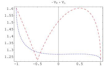
Figure 7: The difference of the $\Delta$ and the Y-string potentials divided by the product of the string tension and the hyper-radius $(V_{\Delta}-V_{\rm Y})/(\sigma R)$, as a function of the cosine of the hyper-angle $z=\cos 2\chi$, at fixed values of $x=\cos\theta=\pm 1$ (red long dashes) and $x=\cos\theta=0$ (blue short dashes). Note that the difference is always (substantially) larger than unity, let alone zero.

This shows that there is no continuous connection between the $\Delta$ and the Y-string potentials at non-zero $R\neq 0$ and equal string tensions $\sigma_{\Delta}=\sigma_{\rm Y}$.

One may try and change the string tensions $\sigma_{\Delta}\neq\sigma_{Y}$, in which case there is an intersection of the two surfaces, but that is not the problem that we started with. We shall return to this new scenario below. Yet, even in that scenario there can be a transition from one to another type of string only in a limited sub-space of shapes.

II.3.2 Difference of string potentials with unequal string tensions $\sigma_{\Delta}\neq\sigma_{\rm Y}$

One may readily circumvent the latter condition and then find some small overlap of the two string potentials, see Figs. 8 and 9. Yet, even then the overlap region is (only) a continuous curve in the $(x,z)$ plane, i.e. it covers a negligibly small (“measure zero”) “number”/set of allowed triangular configurations (“shapes”) as compared with the extent of all possible such sets, described by the complete “shape space” $(x,z)$ plane. Note, moreover, that this overlap lies within the “allowed region” of shape space only in a limited range of values of the ratio $\sigma_{\rm Y}/\sigma_{\Delta}\in(\sqrt{3},1.86)=(1.732,1.86)$. For higher values of this ratio the overlap curve lies partially, or completely (for $\sigma_{\rm Y}/\sigma_{\Delta}>1.96$) outside the range of validity (continuous black line in Fig. 9) of the three-body potential $V_{\rm Y}$, so this solution is essentially irrelevant .

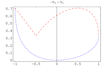
Figure 8: The difference of the $\Delta$ and the Y-string potentials divided by the product of the string tension and the hyper-radius $(V_{\Delta}-V_{\rm Y})/(\sigma R)$, as a function of the cosine of the hyper-angle $z=\cos 2\chi$, at two fixed values of $x=\cos\theta=0,1$ and $\sigma_{\rm Y}/\sigma_{\Delta}=\sqrt{3}=1.732$. Note that the difference vanishes at only one point: $x=0=z$.

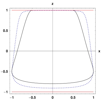
Figure 9: The locus of vanishing difference of the $\Delta$ and the Y-string potentials (blue dashes) as a function of the cosine of the hyper-angle $z=\cos 2\chi$, and $x=\cos\theta$, at $\sigma_{\rm Y}/\sigma_{\Delta}=1.96$. Note that this whole curve lies outside the range of validity (continuous black line) of the three-body potential $V_{\rm Y}$, in which all of the angles are smaller than $120^{o}$.

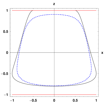
Figure 10: The locus of vanishing difference of the $\Delta$ and the Y-string potentials (blue dashes) as a function of the cosine of the hyper-angle $z=\cos 2\chi$, and $x=\cos\theta$, at $\sigma_{\rm Y}/\sigma_{\Delta}=1.86$. Note that this whole curve lies inside the range of validity (continuous black line) of the three-body potential, in which all of the angles are smaller than $120^{o}$.

III Analytic proof of incompatibility of $\Delta$ and Y-strings

This was just a numerical proof which did not expose the deeper underlying reasons for this incompatibility: the (in)dependence of these two strings on different permutation symmetric variables. For an analytic proof of incompatibility we turn to the study of the permutation symmetry in the three-body potential.

III.0.1 Permutation symmetry properties of the Jacobi coordinates and of the potential

The Jacobi relative coordinate vectors $(\rho,\lambda)$ furnish a two-dimensional irreducible representation of the $S_{3}$ permutation symmetry group. For example, let $P_{ij}$ be the (two-body) $ij$-th particle permutation operator (transposition); then

$$P_{12}\vec{\rho} \rightarrow-\vec{\rho}$$ (18a)

$$P_{12}\vec{\lambda} \rightarrow\vec{\lambda}$$ (18b)

$$P_{13}\vec{\rho} \rightarrow\frac{1}{2}\vec{\rho}-\frac{\sqrt{3}}{2}\vec{\lambda}$$ (18c)

$$P_{13}\vec{\lambda} \rightarrow-\frac{\sqrt{3}}{2}\vec{\rho}-\frac{1}{2}\vec{\lambda}$$ (18d)

Here we see that the $S_{3}$ permutation symmetry implies an invariance (of the potential) under two rotations, through integer multiples of $\frac{2\pi}{3}=120^{\circ}$, and three reflections in the $({\bm{\rho}},{\bm{\lambda}})$ plane.. One special case of such a permutation is the $P_{12}$ transposition, which is a reflection that reverses the sign of $\cos\theta\to-\cos\theta$, which is equivalent to the already mentioned (geometrical) mirror symmetry.

Starting from $({\bm{\rho}},{\bm{\lambda}})$ one can construct one symmetric ${\bf V}$, and two antisymmetric vectors: ${\bf A},{\bf{W}}$.

$${\bf V} = {\bm{\lambda}}\left({\bm{\lambda}}^{2}-{\bm{\rho}}^{2}\right)-2{\bm{\rho}}({\bm{\rho}}\cdot{\bm{\lambda}})$$ (19)

$${\bf A} = {\bm{\rho}}\left({\bm{\lambda}}^{2}-{\bm{\rho}}^{2}\right)+2{\bm{\lambda}}({\bm{\rho}}\cdot{\bm{\lambda}})$$ (20)

$${\bf{W}} = {\bm{\rho}}\times{\bm{\lambda}}.\$$ (21)

The “lengths” (norms) of vectors $V=|{\bf V}|$, $A=|{\bf A}|$, $W=|{\bf W}|$ are invariant under the quark permutations. The hyper-radius squared $R^{2}$ is the fourth permutation invariant scalar. Of course, we expect only three out of four permutation invariant scalars to be (non-linearly) independent. The non-linear relationship reads

$$V^{2}+A^{2} = R^{2}\left[R^{4}-4W^{2}\right],\$$ (22)

so the third permutation symmetric variable may be taken as $(V^{2}-A^{2})$. Any (reasonable) confining three-body potential must be permutation symmetric, so it must be a function of (only) $R,W$ and $(V^{2}-A^{2})$. As all three of these variables have non-zero dimensions, one might think that each one represents a potentially new definition of the “interquark distance”; that is not the case, as can be seen when one changes to hyper-spherical coordinates.

III.0.2 String potentials in terms of symmetrized hyper-spherical coordinates

The three permutation-symmetric hyper-spherical variables are $R$ and

$$W = \frac{1}{2}\,R^{2}\,\sin 2\chi\sin\theta$$ (23)

$$V^{2}-A^{2} = R^{6}\,\cos 2\chi\,\left(\cos^{2}2\chi-3\left(\sin 2\chi\,\cos\theta\right)^{2}\right)\$$ (24)

When the interaction potential does not depend functionally on all three permutation symmetric variables, then additional dynamical symmetries appear: e.g. the “central” part of the string potential Eq. (5),

$$V_{\rm Y} = \sigma\sqrt{\frac{3}{2}R^{2}\left(1+\sin 2\chi\sin\theta\right)}=\sigma\sqrt{\frac{3}{2}\left(R^{2}+2W\right)},\$$ (25)

being a function of only $W$ and $R$, i.e. not a function of $(V^{2}-A^{2})$, is invariant under arbitrary rotations (not just through integer multiples of $\frac{2\pi}{3}=120^{\circ}$) in the $({\bm{\rho}},{\bm{\lambda}})$ plane. That leads to a new integral of motion $G={\bm{\lambda}}\cdot{\bf p_{\rho}}-{\bm{\rho}}\cdot{\bf p_{\lambda}}$, associated with the dynamical symmetry (Lie) group $O(2)$, see Sect. below, which is not conserved in the case of the $\Delta$ string potential. Further, when the potential depends only on $R$, the dynamical symmetry is extended to the $O(6)$ Lie group.

The $\Delta$-string potential

$$V_{\Delta} = \sigma\sum_{i<j=1}^{3}|{\bf x}_{i}-{\bf x}_{j}|$$ (26)

$$= \sigma\left(\sqrt{2}\rho+\sqrt{\frac{3}{2}}\left|{\bm{\lambda}}+\frac{{\bm{\rho}}}{\sqrt{3}}\right|+\sqrt{\frac{3}{2}}\left|{\bm{\lambda}}-\frac{{\bm{\rho}}}{\sqrt{3}}\right|\right)\$$

can be expressed in terms of $({\bf V},{\bf A})$: just solve Eqs. (19),(20) for $({\bm{\rho}},{\bm{\lambda}})$ as functions of $({\bf V},{\bf A})$ and insert the results

$${\bm{\rho}} = \left({\bf V}\left({\bm{\lambda}}^{2}-{\bm{\rho}}^{2}\right)+2{\bf A}({\bm{\rho}}\cdot{\bm{\lambda}})\right)\left(R^{2}-\left(2W\right)^{2}\right)^{-2}$$ (27)

$${\bm{\lambda}} = \left({\bf A}\left({\bm{\lambda}}^{2}-{\bm{\rho}}^{2}\right)-2{\bf V}({\bm{\rho}}\cdot{\bm{\lambda}})\right)\left(R^{2}-\left(2W\right)^{2}\right)^{-2}\$$ (28)

i.e.

$${\bm{\rho}} = \left({\bf V}\cos 2\chi+{\bf A}\left(\sin 2\chi\,\cos\theta\right)\right)\left(1-\left(\frac{2W}{R^{2}}\right)^{2}\right)^{-2}$$ (29)

$${\bm{\lambda}} = \left({\bf A}\cos 2\chi-{\bf V}\left(\sin 2\chi\,\cos\theta\right)\right)\left(1-\left(\frac{2W}{R^{2}}\right)^{2}\right)^{-2}\$$ (30)

into Eq. (26) which shows that

$$V_{\Delta} = V_{\Delta}(R,W,(V^{2}-A^{2}))\$$ (31)

is a function of all three permutation symmetric three-body variables, however. So, we see that in general the two string potentials depend on different symmetric three-body variables, and thus cannot be smoothly connected, except perhaps in special cases/geometries, where the variable $(V^{2}-A^{2})$, and/or other variable(s) vanish.

III.0.3 Admissible region(s) for a “smooth crossover” of two strings

Thus, we need to solve

$$V^{2}-A^{2} = R^{6}\,\cos 2\chi\,\left(\cos^{2}2\chi-3\left(\sin 2\chi\,\cos\theta\right)^{2}\right)=0.\$$ (32)

There are two “trivial” solutions: 1) $R=0$; 2) $\cos 2\chi=0$; and a family of non-trivial solutions to 3) $\cos^{2}2\chi-3\left(\sin 2\chi\,\cos\theta\right)^{2}=0$, i.e. $\cot 2\chi=\pm\sqrt{3}\,|\cos\theta|$, which determines the admissible “smooth crossover” region (the blue long-dashed curve) in Fig. 11.

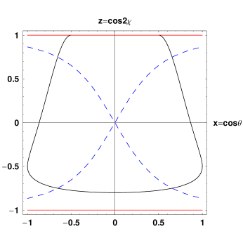
Figure 11: The boundary in the $\chi$ vs. $\theta$ plane (solid line), between the regions in which one of the angles is larger than $120^{o}$, and the curves along which the functional identity of the $\Delta$ and the Y-string potentials is admissible (the blue long-dashed curve).

Thus, we can see that out of the double-continuum (“plane”) of possible geometric configurations at a given “interquark distance” $R$, a “smooth crossover” is potentially admissible, though not guaranteed, only on a single continuum (the blue dashed curves and the vertical axis at $x=0$ in Fig. 11). Now, to make this an actual “smooth crossover” region, rather than merely an admissible one, one must find the intersection of this curve and the locus of zeros of $V_{\Delta}-V_{\rm Y}$, that we searched for in Sect. II.3.1, to no avail.

This fact, together with our numerical results from Sect. II.3.1, are sufficient proof of our claim that even along this curve the crossover is never smooth. This means that, in order to provide a continuous transition from the $\Delta$ to the Y-string configuration at any finite-$R$ crossover point, including the $R=0.8fm$ one, the string tension $\sigma$ must be variable and have a discontinuity in at least one (permutation symmetric) variable. All-in-all, this shows that with constant string tension $\sigma_{\rm Y}=\sigma_{\Delta}$ there can be no smooth transition from the $\Delta$ to the Y-string configuration in any geometry. Even when $\sigma_{\rm Y}/\sigma_{\Delta}\in(1.732,1.86)$ there are only three geometric configurations where a smooth transition can be accomplished, see the discussion below and Fig. 13.

III.0.4 Dynamical symmetry of the Y-string potential

As stated above, independence of the variable $(V^{2}-A^{2})$ leads to the invariance under “generalized rotation”

$$\delta{\bm{\rho}} = \varepsilon{\bm{\lambda}}$$

$$\delta{\bm{\lambda}} = -\varepsilon{\bm{\rho}}.\$$ (33)

in the six-dimensional hyper-space and thus leads to the new integral-of-motion $G={\bm{\lambda}}\cdot{\bf p_{\rho}}-{\bm{\rho}}\cdot{\bf p_{\lambda}}$, associated with the dynamical symmetry (Lie) group $O(2)$ that is a subgroup of the full $O(6)$ Lie group. In certain cases the new integral of motion $G$ can be integrated and the resulting holonomic constraint can be used to eliminate one degree of freedom SD07 . In the case of the $\Delta$ string potential this $G$ is not an integral-of-motion, i.e. it is not constant in time, however, due to the absence of the O(2) symmetry of this potential SD07 . The dynamical O(2) transformation rules Eqs. (33) can be applied to the coordinates $(z,x)$ as follows:

$$\delta x = 2\varepsilon(1-x^{2})\frac{z}{\sqrt{1-z^{2}}}$$

$$\delta z = -2\varepsilon x\sqrt{1-z^{2}}.\$$ (34)

Note that these equations are non-linear in $(x,z)$ implying a non-trivial transformation of the “shape space” under this new dynamical O(2) symmetry. Only near the origin $(x,z)=(0,0)$ does this transformation look like an infinitesimal rotation; at the edges $(x,z)=(\pm 1,\pm 1)$ it either vanishes, or diverges. One can find another set of scalar variables $(x\sqrt{1-z^{2}},z)$ in which the dynamical O(2) symmetry transformation rules Eqs. (33) are linear, but at the price of introducing imaginary parts of the potential, at least in some regions of the “shape space”. A detailed study of this symmetry is a task for the future SD07 .

IV Approximations to the string potentials

IV.1 String approximations to the lattice: the composite string

One possible way to fit the lattice results is, perhaps, to have a “composite Y-string” that contains a “core triangle” of variable size (proportional to, yet smaller than the quark triangle) instead of the Y-junction point, see Fig. 12. In that case, however, one may not talk about a definite cross-over inter-quark distance/hyper-radius, and one would still have contributions from both kinds of string at all distances.

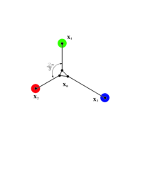
Figure 12: The new three-quark Y-junction string potential.

Note, however, that this prescription is precisely equivalent to the sum of two strings with unequal tensions: for a given (fixed) value of parameter $\alpha\in(0,1)$ (coefficient of proportionality) one has

$$V_{\rm composite}=\alpha V_{\rm Y}+(1-\alpha)V_{\Delta}=\sigma_{\rm Y}\min_{\bf x_{0}}\sum_{i=1}^{3}|{\bf x_{i}}-{\bf x_{0}}|+\sigma_{\Delta}\sum_{i<j}^{3}|{\bf x}_{i}-{\bf x}_{j}|.$$ (35)

There is at least one good reason for the unequal string tensions, viz. the different color factors associated with the quadratic and the cubic Casimir operators of SU(3), c.f. Ref. vd01 . It appears “natural” to associate the cubic Casimir color factor with the Y-string and the quadratic Casimir color factor with the $\Delta$ string. As there is no (reliable) way of dealing with color non-singlets on the lattice (see, however the work of Saito et al. saito05 ) heretofore there was little hope of extracting these factors (or at least their ratio) from the lattice. This Ansatz allows, at least in principle, the extraction of the ratio of the Y-string and the $\Delta$-string tensions $\sigma_{\rm Y}/\sigma_{\Delta}$.

Note that in this case the smooth crossover from the $\Delta$ to the Y-string is not entirely out of the question, albeit it is still severely restricted in the shape space. The intersection of the curve defined by Eq. (32) and the locus of zeros of $V_{\Delta}-V_{\rm Y}$, Figs. 9, 10, yields the allowed crossover points/configurations, of which there are at most six (out of a double-continuum, see Fig. 13), and that only when $\sigma_{\rm Y}/\sigma_{\Delta}\in(1.732,1.86)$. One obtains a region of admissible values of $\alpha$ from the admissible values of $\sigma_{\rm Y}=\alpha\;\sigma$ and $\sigma_{\Delta}=(1-\alpha)\;\sigma$. Then $\sigma_{\rm Y}/\sigma_{\Delta}=\alpha/(1-\alpha)\in(1.732,1.86)$, implies $\alpha\in(0.634,0.650)$. If this turns out too restrictive for the actual lattice results, then one may even introduce a hyper-radially dependent coefficient $\alpha(R)$ that peaks at some non-zero $R$, i.e. a not-quite-linearly rising two-body confining potential.

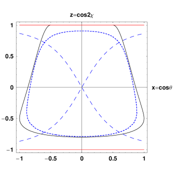
Figure 13: The boundary in the $\chi$ vs. $\theta$ plane (solid line), between the regions in which all of the angles are smaller than $120^{o}$ and the ones where they are not, the locus of zeros of $V_{\Delta}-V_{\rm Y}$ at $\sigma_{\rm Y}/\sigma_{\Delta}=1.86$ (the blue short-dashed curve), and the lines along which identity of the $\Delta$ and the Y-string potentials is admissible (the blue long-dashed curve).

In order to facilitate this separation of the Y-string from the $\Delta$-string, the hyper-angular dependence of the three-body potential ought to be expressed in terms of the new variables $x^{{}^{\prime}}=x\,\sqrt{1-z^{2}}$ and $z^{{}^{\prime}}=z$. Then the Y-string component is manifested through the sole dependence on $\rho^{2}=\,\left(x^{{}^{\prime}2}+\,z^{{}^{\prime}2}\right)=\,(V^{2}+A^{2})R^{-6}=\,\left(1-\,\left(\frac{2W}{R^{2}}\right)^{2}\right)$, whereas the $\Delta$-string is manifested through the dependence of the potential on the new hyperangle $\phi=\tan^{-1}\left(\frac{x^{{}^{\prime}}}{z^{{}^{\prime}}}\right)$, within the confines of the “central potential” boundary (defined by Eqs. (17) in terms of “old” variables $(\chi,\theta)$). If both the Y-string and the $\Delta$-string components are present in the lattice three-body potential, their ratio can be disentangled by measuring the ratio of the $\rho=\,\sqrt{x^{{}^{\prime}2}+\,z^{{}^{\prime}2}}$ to the $\phi=\tan^{-1}\left(\frac{x^{{}^{\prime}}}{z^{{}^{\prime}}}\right)$ dependencies, again within the confines of the “central potential” boundary, because the $\Delta$-string also depends on $\rho$.

Before closing this subsection, we ought to point out that another, perhaps similar in spirit, way to fit the lattice results has been devised and applied in Ref. taka01 . In that “generalized Y-string Ansatz”, a “core circle” of a definite radius has been assumed around the Y-junction point, see Fig. 14 in Ref. taka01 . This Ansatz is rather difficult to describe analytically in terms of hyper-spherical coordinates, so its validity would be difficult to ascertain on the lattice. The “composite string” Ansatz, on the other hand, can be readily recognized by its dependence on the “third variable” which may be chosen either as $(V^{2}-A^{2})\,R^{-6}=\,z\,\left(z^{2}-3\,x^{2}\,\left(1-z^{2}\right)\right)=R^{6}\,z^{{}^{\prime}}\,\left(z^{{}^{\prime}2}-3\,x^{{}^{\prime}2}\right)$, or as $\phi$.

IV.2 Optimal two-body approximation to the “central” Y-string potential

In this light one may try using a linear combination of the Y-string potential and a (linearly) rising two-body potential, perhaps with a variable string tension in the constituent quark model calculations. The Y-string potential has been known for the difficulty of implementation in the Schrödinger equation, which has only recently been solved systematically, see dss09 ,Narodetskii:2008uc , so the authors of Refs. fabr97 ,Grenoble03 tried to approximate the “central” Y-string potential $V_{\rm Y}$ with a two-body $V_{\Delta}$ plus possibly a one-body potential $V_{\rm CM}$, that are easier to deal with numerically. Such approximations may still be valuable in calculations of multi-quark states. Here we show that one particular linear combination of $V_{\Delta}$ and $V_{\rm CM}$

$$V_{\rm comb.} = \frac{1}{2}\left(V_{\rm CM}+\frac{1}{\sqrt{3}}V_{\Delta}\right)=\frac{\sigma}{2}\left(\sum_{i=1}^{3}|{\bf x_{i}}-{\bf x_{\rm CM}}|+\frac{1}{\sqrt{3}}\sum_{i<j}^{3}|{\bf x}_{i}-{\bf x}_{j}|\right),$$ (36)

$$= \sigma\left(\sqrt{\frac{2}{3}}(\rho+\lambda)+\sqrt{\frac{1}{2}}\left(\left|{\bm{\lambda}}+\frac{{\bm{\rho}}}{\sqrt{3}}\right|+\left|{\bm{\lambda}}-\frac{{\bm{\rho}}}{\sqrt{3}}\right|+\left|{\bm{\rho}}+\frac{{\bm{\lambda}}}{\sqrt{3}}\right|+\left|{\bm{\rho}}-\frac{{\bm{\lambda}}}{\sqrt{3}}\right|\right)\right)\$$

assumes the highest degree of dynamical symmetry possible with these variables and a linear hyper-radial dependence, viz. the symmetry under the exchange ${\bm{\rho}}\leftrightarrow{\bm{\lambda}}$, that exceeds the usual $S_{3}$ permutation symmetry.

That new symmetry does not amount to the exact O(2) symmetry of the “central” Y-string potential $V_{\rm Y}$, as yet, but is numerically sufficiently close to it in the region of applicability, see Fig. 14, for most practical purposes, like that of the quark model calculations.

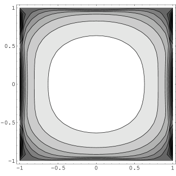
Figure 14: Contour plot of the difference between the genuine Y-string potential $V_{\rm Y}$, shown in Fig. 6, and the combined CM- and $\Delta$-string potentials $\frac{1}{2}\left[V_{\rm CM}+1/{\sqrt{3}}V_{\Delta}\right]$ as a function of the cosine of the hyper-angle $z=\cos 2\chi$, and $x=\cos\theta$. Note that the overall (“quasi-rotational”) symmetry of this figure is the same as that of Fig. 6, except in the corners and near the edges of the square, where the difference is the largest. The darker regions indicate a larger value of the difference of the potentials.

In Fig. 15, we show the difference between the combined CM- and $\Delta$-string potential $\frac{1}{2}\left[V_{\rm CM}+V_{\Delta}\right]$ used in Ref. Grenoble03 . Note the conspicuous broadening of the contour in the lower half-plane (the pear-shape of the contours) and consequently the absence of the continuous “quasi-rotational” symmetry in this figure, which goes to show that this approximation to the genuine Y-string potential does not have the correct symmetry, which in turn is a consequence of the missing factor $1/{\sqrt{3}}$.

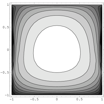
Figure 15: Contour plot of the difference between the genuine Y-string potential $V_{\rm Y}$ and the combined CM- and $\Delta$-string potential $\frac{1}{2}\left[V_{\rm CM}+V_{\Delta}\right]$ used in Ref. Grenoble03 as a function of the cosine of the hyper-angle $z=\cos 2\chi$, and $x=\cos\theta$. Note that the overall (“quasi-rotational”) symmetry of this figure is broken as compared with that of Fig. 6, due to the missing factor $1/{\sqrt{3}}$. The difference is the largest in the darkest regions.

V Summary and Discussion

In summary, we have studied the functional dependence of the three-quark confining potential due to a Y-string, and the $\Delta$-string. We have found fundamentally different results for these two kinds of strings, which lead to different constants of the motion (“universality classes”). This means that there can be no smooth crossover between the two, except at the vanishing hyper-radius $R$, which is physically singular and mathematically not very meaningful. Perhaps, this should be no surprise, as the two strings have different topologies: one separates the plane into two disjoint parts, whereas the other one does not.

References

- (1) X. Artru, Nucl. Phys. B 85, 442 (1975).
- (2) H. G. Dosch and V. Mueller, Nucl. Phys. B 116, 470 (1976).
- (3) T. T. Takahashi, H. Matsufuru, Y. Nemoto, and H. Suganuma, Phys. Rev. Lett. 86, 18 (2001); Phys. Rev D 65, 114509 (2002).
- (4) C. Alexandrou, P. De Forcrand, A. Tsapalis, Phys. Rev. D 65, 054503,(2002).
- (5) H. Iida, N. Sakumichi and H. Suganuma, arXiv:0810.1115 [hep-lat].
- (6) V. G. Bornyakov et al. [DIK Collaboration], Phys. Rev. D 70, 054506 (2004) [arXiv:hep-lat/0401026].
- (7) M. Caselle, G. Delfino, P. Grinza, O. Jahn and N. Magnoli, J. Stat. Mech. 0603, P008 (2006) [arXiv:hep-th/0511168].
- (8) Ph. de Forcrand and O. Jahn, Nucl. Phys. A 755, 475 (2005) [arXiv:hep-ph/0502039].
- (9) V. Dmitrašinovi\a’ c, T. Sato and M. Suvakov, Eur. Phys. J. C 62, 383-398 (2009); see also V. Dmitrašinovi\a’ c, T. Sato and M. Šuvakov, “Low-lying states in the Y-string three-quark potential”, p. 30 - 35, Proceedings of the Mini-Workshop “Few-Quark states and the Continuum”, “Bled Workshops in Physics”, Vol. 9, No. 9. ed. B. Golli, M. Rosina and S. Širca, DMFA - Založništvo, Ljubljana, Slovenia, (2008).
- (10) I. M. Narodetskii, C. Semay and A. I. Veselov, Eur. Phys. J. C 55, 403 (2008)
- (11) Yu. A. Simonov, Sov. J. Nucl. Phys. 3, 461 (1966) [Yad. Fiz. 3, 630 (1966)].
- (12) V. Dmitrašinović, Phys. Lett. B 499, 135 (2001); Phys. Rev. D 67, 114007 (2003).
- (13) A. Nakamura, T. Saito, Phys. Lett. B 621, 171 (2005).
- (14) M. Fabre de la Ripelle and M. Lassaut, Few-Body Systems 23, 75 (1997).
- (15) B. Silvestre-Brac, C. Semay, I. M. Narodetskii, and A.I. Veselov, Eur.Phys.J. C32, 385 (2003). I.M. Narodetskii and M.A. Trusov, hep-ph/0307131v1.
- (16) V. Dmitrašinović and M. Šuvakov, in preparation (2009).