Generalized Voronoi Partition Based Multi-Agent Search using Heterogeneous Sensors

Abstract

In this paper we propose search strategies for heterogeneous multi-agent systems. Multiple agents, equipped with communication gadget, computational capability, and sensors having heterogeneous capabilities, are deployed in the search space to gather information such as presence of targets. Lack of information about the search space is modeled as an uncertainty density distribution. The uncertainty is reduced on collection of information by the search agents. We propose a generalization of Voronoi partition incorporating the heterogeneity in sensor capabilities, and design optimal deployment strategies for multiple agents, maximizing a single step search effectiveness. The optimal deployment forms the basis for two search strategies, namely, heterogeneous sequential deploy and search and heterogeneous combined deploy and search. We prove that the proposed strategies can reduce the uncertainty density to arbitrarily low level under ideal conditions. We provide a few formal analysis results related to stability and convergence of the proposed control laws, and to spatial distributedness of the strategies under constraints such as limit on maximum speed of agents, agents moving with constant speed and limit on sensor range. Simulation results are provided to validate the theoretical results presented in the paper.

I Introduction

I-A Multi-agent systems

Solving complex problems requires higher intelligence, which nature has gifted to human beings. An alternative to higher individual intelligence is cooperation among individuals with limited intelligence. Such group intelligence is exhibited in nature by swarms of bees, flocks of birds, schools of fish etc. In these, and in myriad such examples from nature, the key factor is cooperation with limited, local, and noisy communication among individuals in a large group. The individuals are governed by a set of simple behavior leading to a more complex and useful emergent group behavior. Honey bees’ nests, territories of the male Tilapia Mossambica etc., exhibit a kind of locational optimization which can be interpreted in terms of centroidal Voronoi configurations [1]. This kind of optimal behavior is also an outcome of a set of rudimentary decisions by individuals with local interactions.

Inspired by nature, scientists and engineers have developed the concept of multi-agent systems with robots, UAVs, etc., as agents. These multi-agent systems can perform a wide variety of tasks such as search and rescue, surveillance, achieve and maintain spatial formations, move as flocks while avoiding obstacles, multiple source identification and several other tasks.

I-B Search using multiple agents

One of the very useful application of multi-agent systems is search and surveillance. Searching for the presence of targets of interest, survivors in a disaster, or information of interest in a large, possibly un-mapped geographical area, is an interesting and practically useful problem. The problem of searching for targets in unknown environments has been addressed in the literature in the past under restrictive conditions [2]-[5]. These seminal contributions were mostly theoretical in nature and were applicable to a single agent searching for single or multiple, and static or moving, targets. Cooperative search by multiple agents have been studied by various researchers. Enns et al. [6] use predefined lanes prioritizing them with the probability of existence of the target. The vehicles cooperate in that the total path length covered by them is minimized while exhaustively searching the area. A dynamic inversion based control law is used to make the vehicles follow the assigned tracks or lanes while considering the maximum turn radius constraint. Spires and Goldsmith [7] use space filling curves such as Hilbert curves to cover a given space and perform exhaustive search by multiple robots. Vincent and Rubin [8] address the problem of cooperative search strategies for unmanned aerial vehicles (UAVs) searching for moving, possibly evading, targets in a hazardous environment. They use predefined swarm patterns with an objective of maximizing the target detection probability in minimum expected time and using minimum number of UAVs having limited communication range. Beard and McLain [9] develop strategies for a team of cooperating UAVs to visit regions of opportunity without collision while avoiding hazards in a search area using dynamic programming methods. The UAVS are also required to stay within communication range of each other. Flint et al. [10] provide a model and algorithm for path planning of multiple UAVs searching in an uncertain and risky environment, also using a dynamic programming approach. For this purpose, the search area is divided into cells and in each cell the probability of existence of a target is defined. Pfister [11] uses fuzzy cognitive map to model the cooperative control process in an autonomous vehicle. In [12]-[14] the authors use distributed reinforcement learning and planning for cooperative multi-agent search. The agents learn about the environment online and store the information in the form of a search map and utilize this information to compute online trajectories. The agents are assumed to be having limitation on maneuverability, sensor range and fuel. In [13] the authors show a finite lower bound on the search time. Rajnarayan and Ghose [15] use concepts from team theory to formulate multi-agent search problems as nonlinear programming problems in a centralized perfect information case. The problem is then reformulated in a Linear-Quadratic-Gaussian setting that admits a decentralized team theoretic solution. Dell et al. [16] develop an optimal branch-and-bound procedure with heuristics such as combinatorial optimization, genetic algorithm and local start with random restarts, for solving constrained-path problems with multiple searchers. Sujit and Ghose [17] use concepts of graph theory and game theory to solve the problem of coordinated multi-agent search. They partition the search space into hexagonal cells and associate each cell with an uncertainty value representing lack of information about the cell. As the agents move through these cells, they acquire information, reducing the corresponding uncertainty value. Jin et al. [18] address a search and destroy mission problem in a military setting with heterogeneous team of UAVs.

Mobile agents equipped with sensors to gather information about the search area form a sensor network. Optimal deployment of these sensors or agents carrying sensors which is referred to as “sensor coverage” in the literature, is an important step in achieving effective search. Voronoi partition and its variations are used in sensor network literature. We review the concept of Voronoi partition and some literature on multi-agent systems using this concept.

I-C Voronoi partition in sensor network and multi-agent systems

Voronoi partition (named after Georgy Voronoi [19]), also called Dirichlet tessellation (named after Gustav Lejeune Dirichlet [20]), is a widely used scheme of partitioning a given space based on the concept of “nearness” of objects such as points in a set to some finite number of pre-defined locations in the set. In its standard setting Euclidean distance is used as a measure of “nearness” (see [21] for a survey). This concept finds application in many fields such as CAD, image processing [22, 23] and sensor coverage [24, 25]. There are various generalization of the Voronoi decomposition such as weighted Voronoi partitions and Voronoi partition based on non-Euclidean metric. The dual of Voronoi diagram is the Delaunay graph (named after Boris Delaunay [26]). These two concepts are very useful in multi-agent search.

A class of problems known as locational optimization (or facility location) [27, 28], is used in many applications. These concepts have been used in sensor coverage literature for optimal deployment of sensors. Centroidal Voronoi configuration is a standard solution for this class of problems [29], where the optimal configuration of agents is the centroids of the corresponding Voronoi cells. Cortes et al. [24, 25] use these concepts to solve a spatially distributed optimal deployment problem for multi-agent systems. A density distribution, as a measure of the probability of occurrence of an event along with a function of the Euclidean distance providing a quantitative assessment of the sensing performance, is used to formulate the problem. Centroidal Voronoi configuration, with centroid of a Voronoi cell, computed based on the density distribution within the cell, is shown to be the optimal deployment of sensors minimizing the sensory error. The Voronoi partition becomes the natural optimal partitioning due to monotonic variation of sensor effectiveness with the Euclidean distance. Schwager et al. [30] interpret the density distribution of [25] in a non-probabilistic framework and approximate it by sensor measurements. Pimenta et al. [31] follow a similar approach to address problem with heterogeneous robots. They let the sensors to be of different types (in the sense of having different footprints) and relax the point robots assumptions. Generalization of Voronoi partition such as power diagrams (or Voronoi diagram in Laguerre geometry) are used to account for different footprints of the sensors (assumed to be discs). Due to assumption of finite size of robots, the robots are assumed to be discs and a free Voronoi region is defined. A constrained locational optimization problem is solved. They also extend the results to non-convex environments. Ma et al. [32] use an adaptive triangulation (ATRI) algorithm based on the Delaunay triangulation [26], which is a dual of the Voronoi partition, with length of the Delaunay edge as a parameter, to achieve non-uniform coverage.

In [33]-[35] authors address a problem of searching an unknown area with a priori known uncertainty distribution using multiple agents. The concept of Voronoi partition was used in formulating optimal deployment strategies for multiple agents maximizing the search effectiveness.

I-D Motivation and contribution of the paper

In the literature on multi-agent search, it is largely assumed that the agents and the sensors are homogeneous in nature. But this assumption may not be valid in many practical applications. It is most likely that the sensors will have varied capabilities in terms of the strength and range, making the problem heterogenous in nature. We address this issue in this paper, and formulate and solve a heterogeneous multi-agent search problem. In order to solve this problem, we present a generalization of the standard Voronoi partition and use it to design an optimal deployment of heterogeneous agents.

The generalization of the Voronoi partition proposed in this work takes into account the heterogeneity in the sensors’ capabilities, in order to design an optimal deployment strategy for heterogeneous agents. The agent locations are used as sites or nodes and a concept of a node function, which is the sensor effectiveness function associated with each node is introduced in place of the usual distance measure. The standard Voronoi partition and many of its variations can be obtained from this generalization.

In [24, 25, 30] authors use Voronoi partitions for optimal deployment of homogeneous sensors and [31] use power diagrams for the case of heterogeneous agents. In [33]-[35], authors use Voronoi partition to design multi-agent search strategies for agents with homogeneous sensors. In this paper, we generalize these concepts and incorporate the sensors with heterogeneous capabilities. The optimal deployment strategy is developed based on the generalized Voronoi partition maximizing the search effectiveness in a given step and forms the basis for two heterogeneous multi-agent search strategies namely, heterogeneous sequential deploy and search and heterogeneous combined deploy and search. We provide convergence results for the search strategies and also analyze the strategies for spatial distributedness property. Some preliminary results using heterogeneous sensors have been earlier reported in [36]. The concepts developed in this work are based on and generalization of those provided in [33],[34].

I-E Organization of the paper

The paper is organized as follows. We preview a few mathematical concepts used in this work in Section II. In Section III we provide a generalization of Voronoi partition. In Section IV we formulate a heterogeneous multi-agent search problem. The multi-center objective function, its critical points, the control law responsible for motion of agents, and its convergence and spatial distributedness property are also discussed here. In Section V we impose a few constraints on the agents’ speeds and provide the convergence proof for the agents’ trajectories with the corresponding control laws. In Section VI we propose and analytically study the heterogeneous sequential deploy and search strategy. In Section VII we propose and analyze the heterogeneous combined deploy and search strategy. We study the effect of limit on sensor range in Section VIII and discuss a few implementation issues in Section IX. Simulation results and discussions are provided in Section X, and finally the paper concludes in Section XI with possible directions for future work.

II Mathematical preliminaries

In this section we preview mathematical concepts such as LaSalle’s invariance principle and Liebniz theorem used in the present work.

II-A LaSalle’s invariance principle

Here we state LaSalle’s invariance principle [37, 38] used widely to study the stability of nonlinear dynamical systems. We state the theorem as in [39] (Theorem 3.8 in [39]).

Consider a dynamical system in a domain $D$

$$\dot{x}=f(x)\text{, }f:D\rightarrow\mathbb{R}^{d}$$ (1)

Let $V:D\rightarrow\mathbb{R}$ be a continuously differentiable function and assume that (i) $M\subset D$ is a compact set, invariant with respect to the solutions of (1); (ii) $\dot{V}\leq 0$ in $M$; (iii) $E:\{x:x\in M\text{, and }\dot{V}(x)=0\}$; that is, $E$ is set of all points of $M$ such that $\dot{V}(x)=0$; and (iv) $N$ is the largest invariant set in $E$. Then every solution of (1) starting in $M$ approaches $N$ as $t\rightarrow\infty$.

Here by invariant set we mean that if the trajectory is within the set at some time, then it remains within the set for all time. Important differences of the LaSalle’s invariance principle as compared to the Lyapunov Theorem are (i) $\dot{V}$ is required to be negative semi-definite rather than negative definite and (ii) the function $V$ need not be positive definite (see Remark on Theorem 3.8 in [39], pp 90-91).

II-B Leibniz theorem and its generalization

The Leibniz theorem is widely used in fluid mechanics [40], and shows how to differentiate an integral whose integrand as well as the limits of integration are functions of the variable with respect to which differentiation is done. The theorem gives the formula

$$\frac{d}{dy}\int_{a(y)}^{b(y)}F(x,y)dx=\int_{a}^{b}\frac{\partial F}{\partial y}dx+\frac{db}{dy}F(b,y)-\frac{da}{dy}F(a,y)$$ (2)

Eqn. (2) can be generalized for a $d$-dimensional Euclidean space as

$$\frac{d}{dy}\int_{\mathcal{V}(y)}F(x,y)d\mathcal{V}=\int_{\mathcal{V}}\frac{\partial F}{\partial y}d\mathcal{V}+\int_{\mathbf{S}}\mathbf{n}(x).\mathbf{u}(x)FdS$$ (3)

where, $\mathcal{V}\subset\mathbb{R}^{d}$ is the volume in which the integration is carried out, $d\mathcal{V}$ is the differential volume element, $\mathbf{S}$ is the bounding hypersurface of $V$, $\mathbf{n}(x)$ is the unit outward normal to $\mathbf{S}$ and $\mathbf{u}(x)=\frac{d\mathbf{S}}{dy}(x)$ is the rate at which the surface moves with respect to $y$ at $x\in\mathbf{S}$.

III Generalization of the Voronoi partition

Here we present a generalization of the Voronoi partition considering the heterogeneity in the sensors’ capabilities. Voronoi partition [19, 20] is a widely used scheme of partitioning a given space and finds applications in many fields such as CAD, image processing and sensor coverage. We can find several extensions or generalizations of Voronoi partition to suit specific applications [21, 23, 28]. Herbert and Seidel [41] have introduced an approach in which, instead of the site set, a finite set of real-valued functions $f_{i}:D\mapsto\mathbb{R}$ is used to partition the domain $D$. Standard Voronoi partition and other known generalizations can be extracted from this abstract general form.

In this paper we define a generalization of the Voronoi partition to suit our application, namely the heterogeneous multi-agent search. We use, (i) the search space as the space to be partitioned, (ii) the site set as the set of points in the search space which are the positions of the agents in it, and (iii) a set of node functions in place of a distance measure.

Consider a space $Q\subset\mathbb{R}^{d}$, a set of points called nodes or generators $\mathcal{P}=\{p_{1},p_{2},\ldots,p_{N}\}$, $p_{i}\in Q$, with $p_{i}\neq p_{j}$, whenever $i\neq j$, and monotonically decreasing analytic functions [42] $f_{i}:\mathbb{R}^{+}\mapsto\mathbb{R}$, where $f_{i}$ is called a node function for the $i$-th node. Define a collection $\{V_{i}\}$, $i\in\{1,2,\ldots,N\}$, with mutually disjoint interiors, such that $Q=\cup_{i\in\{1,2,\ldots,N\}}V_{i}$, where $V_{i}$ is defined as

$$V_{i}=\{q\in Q|f_{i}(\|p_{i}-q\|)\geq f_{j}(\|p_{j}-q\|)\quad\forall j\neq i\text{,}\quad j\in\{1,2,\ldots,N\}\}$$ (4)

We call $\{V_{i}\}$, $i\in\{1,2,\ldots,N\}$, as a generalized Voronoi partition of $Q$ with nodes $\mathcal{P}$ and node functions $f_{i}$. In the standard definition of the Voronoi partition, $f_{i}(\|p_{i}-q\|)\geq f_{j}(\|p_{j}-q\|)$ is replaced by $(\|p_{i}-q\|)\leq(\|p_{j}-q\|)$. Note that,

• $V_{i}$ can be topologically non-connected and may contain other Voronoi cells.

• In the context of multi-agent search problem discussed in this paper, $q\in V_{i}$ means that the $i$-th agent is the most effective in performing search task at point $q$. This is reflected in the $\geq$ sign in the definition. In standard Voronoi partition used for the homogeneous multi-agent search, $\leq$ sign for distances ensured that $i$-th agent is most effective in $V_{i}$

• The condition that $f_{i}$ are analytic implies that for every $i,j\in\{1,2,\ldots,N\}$, $f_{i}-f_{j}$ is analytic. By the property of real analytic functions [42], the set of intersection points between any two node functions is a set of measure zero. This ensures that the intersection of any two cells is a set of measure zero, that is, the boundary of a cell is made up of the union of at most $d-1$ dimensional subsets of $\mathbb{R}^{d}$. Otherwise the requirement that the cells should have mutually disjoint interiors may be violated. Analyticity of the node functions $f_{i}$ is a sufficient condition to discount this possibility.

• The standard Voronoi partition and its generalizations such as multiplicatively and additively weighted Voronoi partitions can be extracted as special cases of the proposed generalization.

Theorem 1

The generalized Voronoi partition depends at least continuously on $\mathcal{P}$.

Proof:  If $V_{i}$ and $V_{j}$ are adjacent cells, then all the points $q\in Q$ on the boundary common to them are given by $\{q\in Q|f_{i}(\|p_{i}-q\|)=f_{j}(\|p_{j}-q\|)\}$, that is, the intersection of corresponding node functions. Let the $j$-th agent moves by a small distance $dp$. This makes the common boundary between $V_{i}$ and $V_{j}$ move by a distance, say $dx$. Now as the node functions are monotonically decreasing and are continuous, it is easy to see that $dx\rightarrow 0$ as $dp\rightarrow 0$. This is true for any pair $i$ and $j$. Thus, the Voronoi partition depends continuously on $\mathcal{P}=\{p_{1},p_{2},\ldots,p_{N}\}$. $\Box$

Generalized Delaunay graph

Delaunay graph is the dual of Voronoi partition. Two nodes are said to be neighbors (connected by an edge), if the corresponding Voronoi cells are adjacent. This concept can be extended to generalized Voronoi partitioning scheme. For the sake of simplicity we call such a graph a Delaunay graph, $\mathcal{G}_{D}$. Note that the generalized Delaunay graph, in general, need not have the property of Delaunay triangulation, in fact, it need not even be a triangulation.

Two nodes are said to be neighbors in a generalized Delaunay graph, if the corresponding generalized Voronoi cells are adjacent, that is, $(i,j)\in\mathcal{E}_{\mathcal{G}_{D}}$, the edge set corresponding to the graph $\mathcal{G}_{D}$, if $V_{i}\cap V_{j}\neq\emptyset$.

IV Heterogeneous Multi-Agent Search

In this section we discuss the problem addressed in this paper. $N$ agents are deployed in the search space $Q\subset\mathbb{R}^{d}$, a convex polytope, where, lack of information is modeled as an uncertainty density distribution $\phi:Q\mapsto[0,1]$, a continuous function in $Q$. $P(t)=\{p_{1}(t),p_{2}(t),\ldots,p_{N}(t)\}$, $p_{i}(t)\in Q$ denotes the configuration of the multi-agent system at time $t$, $p_{i}(t)$ denotes the position of the $i$-th agent at time $t$. In future, for convenience, we drop the variable $t$ and refer to the positions by just $p_{i}$. The agents are assumed to have sensors with varied strength and range, whose effectiveness at a point reduces with distance. The agents get deployed in $Q$, perform search, thereby reducing the uncertainty, and we are looking for optimal utilization of the agents to reduce the uncertainty $\phi(q)$ at each point $q\in Q$ below a specified level.

At each iteration, after deploying themselves optimally, the sensors gather information about $Q$, reducing the uncertainty density as,

$$\phi_{n+1}(q)=\phi_{n}(q)\min_{i}\{\beta_{i}(\|p_{i}-q\|)\}$$ (5)

where, $\phi_{n}(q)$ is the density function at the $n$-th iteration; $\beta:\mathbb{R}\mapsto[0,1]$ is a function of the Euclidian distance of a given point in space from the agent, and acts as the factor of reduction in uncertainty by the sensors; and $p_{i}$ is the position of the $i$-th sensor. At a given $q\in Q$, only the agent with the smallest $\beta_{i}(\|p_{i}-q\|)$, that is, the agent which can reduce the uncertainty by the largest amount, is active. If any agent searches within its Voronoi cell, then the updating function (5) gets implemented automatically, That is, the function $\min_{i}\{\beta_{i}(\|p_{i}-q\|)\}$ is simply $\beta_{i}(\|p_{i}-q\|)$, where $p_{i}\in V_{i}$. Usually, sensors’ effectiveness decreases with Euclidean distance, thus $\beta_{i}$, which represents the search effectiveness of $i$-th sensor, can be assumed to be a monotonically increasing analytic function of the Euclidean distance. Equation (5) selects the agent $i$, which is most effective in performing search task at point $q\in Q$. We will discuss more about the function $\beta_{i}$ in a later section.

Note that the condition that $\phi_{0}$ is continuous ensures that $\phi_{n}$ is continuous for all $n$ as $\beta_{i}$ are continuous and at any point $q\in Q$, and on the boundary of generalized Voronoi cells corresponding to any pair of agents $i$ and $j$, $\beta_{i}(\|p_{i}-q\|)=\beta_{j}(\|p_{j}-q\|)$, by the definition of the generalized Voronoi partition.

IV-A Objective function

Now suppose that the agents have to be deployed in $Q$ in such a way as to maximize one-step uncertainty reduction, that is, maximize the effectiveness of one-step of multi-agent search. Consider the objective function for the $n$-th search step,

$$\mathcal{H}^{n} = \int_{Q}\Delta\phi_{n}(q)dQ=\int_{Q}(\phi_{n}(q)-\min_{i}\{\beta_{i}(\|p_{i}-q\|)\}\phi_{n}(q))dQ$$ (6)

$$= \sum_{i}\int_{V_{i}}\phi_{n}(q)(1-\beta_{i}(\|p_{i}-q\|))dQ=\sum_{i}\int_{V_{i}}\phi_{n}(q)f_{i}(r_{i})dQ$$

where, $V_{i}$ is the generalized Voronoi cell given by (4) corresponding to the $i$-th agent, with $f_{i}(.)=1-\beta_{i}(.)$, a monotonically decreasing analytic function as node function, $\mathcal{P}$ as the set of nodes, and $r_{i}=\|p_{i}-q\|$. Below we provide a result which will be useful in obtaining the critical points of the objective function (6).

Lemma 1

The gradient of the multi-center objective function (6) with respect to $p_{i}$ is given by

$$\frac{\partial\mathcal{H}^{n}}{\partial p_{i}}=\int_{V_{i}}\phi(q)\frac{\partial f_{i}(r_{i})}{\partial p_{i}}dQ$$ (7)

where $r_{i}=\|q-p_{i}\|$.

Proof.  Let us rewrite (6) as

$$\mathcal{H}^{n}=\sum_{i\in\{1,2,\ldots N\}}\mathcal{H}^{n}_{i}$$ (8)

where $\mathcal{H}^{n}_{i}=\int_{V_{i}}f_{i}(r_{i})\phi(q)dQ$. Now,

$$\frac{\partial\mathcal{H}^{n}}{\partial p_{i}}=\sum_{j\in\{1,2,\ldots N\}}\frac{\partial\mathcal{H}^{n}_{j}}{\partial p_{i}}$$ (9)

Applying the general form of the Leibniz theorem [40]

$$\frac{\partial\mathcal{H}^{n}}{\partial p_{i}} = \int_{V_{i}}\phi(q)\frac{\partial f_{i}}{\partial p_{i}}(r_{i})dQ+\sum_{j\in N_{i}}\int_{A_{ij}}\mathbf{n}_{ij}(q).\mathbf{u}_{ij}(q)\phi(q)f_{i}(r_{i})dQ$$

$$+\sum_{j\in N_{i}}\int_{A_{ji}}\mathbf{n}_{ji}(q).\mathbf{u}_{ji}(q)\phi(q)f_{j}(r_{j})dQ$$

where, $N_{i}$ is the set of indices of agents which are neighbors of the $i$-th agent in $\mathcal{G}_{D}$, the generalized Delaunay graph, $A_{ij}$ is the part of the bounding surface common to $V_{i}$ and $V_{j}$, $\mathbf{n}_{ij}(q)$ is the unit outward normal to $A_{ij}$ at $q\in A_{ij}$, $\mathbf{u}_{ij}(q)=\frac{dA_{ij}}{dp_{i}}(q)$, the rate of movement of the boundary at $q\in A_{ij}$ with respect to $p_{i}$.

Note that i) $\mathbf{n}_{ij}(q)=-\mathbf{n}_{ji}(q)$, $\forall q\in A_{ij}$, ii) $\mathbf{u}_{ij}(q)=\mathbf{u}_{ji}(q)$, iii) $f_{i}(r_{i})=f_{j}(r_{j})$, $\forall q\in A_{ij}$, by definition of the generalized Voronoi partition, and iv) $\phi$ is continuous. Thus, it is clear that for each $j\in N_{i}$, $\int_{A_{ij}}\mathbf{n}_{ij}(q).\mathbf{u}_{ij}(q)\phi(q)f_{i}(r_{i})dQ=-\int_{A_{ji}}\mathbf{n}_{ji}(q).\mathbf{u}_{ji}(q)\phi(q)f_{j}(r_{j})dQ$, and hence, the last two terms in (IV-A) cancel each other. $\Box$

IV-B The critical points

The gradient of the objective function (6) with respect to $p_{i}$, the location of the $i$-th node in $Q$, can be determined using (7) (by Lemma 1) as

$$\frac{\partial\mathcal{H}^{n}}{\partial p_{i}} = \int_{V_{i}}\phi(q)\frac{\partial f_{i}(r_{i})}{\partial p_{i}}dQ=\int_{V_{i}}\phi(q)\frac{\partial f_{i}(r_{i})}{\partial{(r_{i})}^{2}}(p_{i}-q)dQ$$

$$= -\int_{V_{i}}\tilde{\phi}(q)(p_{i}-q)dQ=-\tilde{M}_{V_{i}}(p_{i}-\tilde{C}_{V_{i}})$$

where, $r_{i}=\|q-p_{i}\|$ and $\tilde{\phi}(q)=-\phi(q)\frac{\partial f_{i}(r_{i})}{\partial{(r_{i})}^{2}}$. As $f_{i},i\in\{1,2,\ldots,N\}$ is strictly decreasing, $\tilde{\phi}(q)$ is always non-negative. Here $\tilde{M}_{V_{i}}$ and $\tilde{C}_{V_{i}}$ are interpreted as the mass and centroid of the cell $V_{i}$ with $\tilde{\phi}$ as density. Thus, the critical points are $p_{i}=\tilde{C}_{V_{i}}$, and such a configuration $\mathcal{P}$, of agents is called a generalized centroidal Voronoi configuration.

Theorem 2

The gradient, given by (IV-B), is spatially distributed over the generalized Delaunay graph $\mathcal{G}_{D}$.

Proof.  The gradient (IV-B) with respect to $p_{i}\in\mathcal{P}$, the present configuration, depends only on the corresponding generalized Voronoi cell $V_{i}$ and values of $\phi$ and the gradient of $f_{i}$ within $V_{i}$. The Voronoi cell $V_{i}$ depends only on the neighbors of $p_{i}$ in $\mathcal{G}_{D}$. Thus, the gradient (IV-B) can be computed with only local information, that is, the neighbors of $p_{i}$ in $\mathcal{G}_{D}$. $\Box$

The critical points are not unique, as with the standard Voronoi partition. But in the case of a generalized Voronoi partition, some of the cells could become null and such a condition can lead to local maxima.

IV-C Selection of $\beta_{i}$

The function $\beta_{i}:\mathbb{R}\mapsto[0,1]$ is a sensor detection function corresponding to the $i$-th agent. The effectiveness of most sensors decreases with the Euclidean distance. Consider

$$\beta_{i}(r)=1-k_{i}e^{-\alpha_{i}{r_{i}}^{2}},\qquad k_{i}\in(0,1)\quad\text{and $\alpha_{i}>0$}$$ (11)

Here, $k_{i}e^{-\alpha_{i}{r_{i}}^{2}}$ represents the effectiveness of the $i$-th sensor which is maximum at ${r_{i}}=0$ and tends to zero as $r\rightarrow\infty$ and $\beta_{i}$ is minimum at ${r_{i}}=0$ (effecting maximum reduction in $\phi$) and tends to unity as $r\rightarrow\infty$ (change in $\phi$ reduces to zero as $r$ increases). Most sensors’ effectiveness reduces over distance as the signal to noise ratio increases. Thus $\beta_{i}$, which is upside down Gaussian, can model a wide variety of sensors with two tunable parameters $k_{i}$ and $\alpha_{i}$.

IV-D Special cases

Here we discuss a few interesting detection functions.

Case 1: $\beta_{i}(r_{i})=1-ke^{-\alpha_{i}r_{i}^{2}}$

Here we consider exponential sensor effectiveness and assume that the parameter $\alpha$ is different for different sensors while $k$ remains the same for all of them, that is, all the agents have sensors with the same maximum effectiveness with different sensor reach (Figure 1 (a)). This case leads to multiplicatively weighted Voronoi partition. The Voronoi cells can be non-connected and also can have one or more Voronoi cells embedded within a cell. Within $V_{i}$, $\tilde{\phi}_{n}(\cdot)=-\alpha_{i}\phi_{n}(\cdot)ke^{-\alpha_{i}r_{i}^{2}}$.

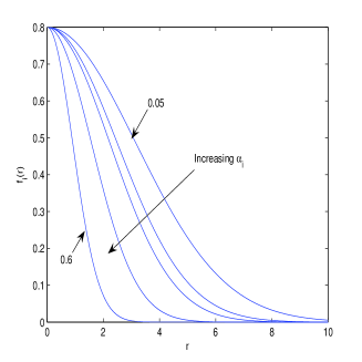
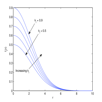
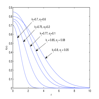
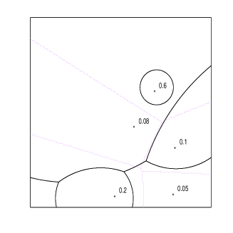
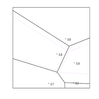
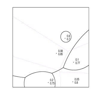
Figure 1: The sensor effectiveness $\beta_{i}(r)=1-k_{i}e^{-\alpha_{i}r_{i}^{2}}$ with a) varying $\alpha_{i}$, b) varying $k_{i}$, and c) both $\alpha_{i}$ and $k_{i}$ varying. d), e), and f) are the corresponding Voronoi partitions with ’*’ showing the locations of nodes or sites, the numbers indicating the parameters, and dotted lines showing the standard Voronoi partition.

Figure 1 (d) shows a Voronoi partition for this case with $k=0.8$. The parameter $k$ does not affect the Voronoi partition. It is easy to show that the partition is a multiplicatively weighted Voronoi partition with weights $\sqrt{\alpha_{i}}$. The Voronoi cell corresponding to node with $\alpha_{i}=0.6$, the highest $\alpha_{i}$ among all the nodes, implying that it is the least effective, is embedded within the cell corresponding to the node with $\alpha_{i}=0.08$, the smallest value, and hence the most effective. The Voronoi cell corresponding to the node with $\alpha_{i}=0.05$ is actually two cells separated by the cell corresponding to node with $\alpha_{i}=0.2$.

Case 2. $\beta_{i}(r_{i})=1-k_{i}e^{-\alpha r_{i}^{2}}$

Here we let the parameter $k_{i}$ be different for different sensors while keeping the value of $\alpha$ same. The agents in this case have sensors with varying maximum effectiveness (Figure 1 (b)). Within $V_{i}$, $\tilde{\phi}_{n}(\cdot)=-\alpha\phi_{(}\cdot)k_{i}e^{-\alpha r_{i}^{2}}$.

Theorem 3

For $Q\subset\mathbb{R}^{2}$, the boundaries of Voronoi cells corresponding to the case $\beta_{i}(r)=1-k_{i}e^{-\alpha r^{2}}$ are straight line segments.

Proof.  Let $q=(x,y)^{\prime}$ be a point on the boundary of cells $V_{i}$ and $V_{j}$. Then we have,

$$k_{1}e^{-\alpha(\parallel p_{1}-q\parallel)^{2}}=k_{2}e^{-\alpha(\parallel p_{2}-q\parallel)^{2}}$$ (12)

Now let $p_{1}=(p_{11},p_{12})^{\prime}$ and $p_{2}=(p_{21},p_{22})^{\prime}$. Solving for $q$ from (12) gives,

$$y=\frac{(p_{11}-p_{21})}{(p_{22}-p_{12})}x+\frac{(1/\alpha)ln(k_{1}/k_{2})+(p_{21}^{2}+p_{22}^{2})-(p_{11}^{2}+p_{12}^{2})}{2(p_{22}-p_{12})}=Mx+C$$ (13)

where, $M$ and $C$ are constants for a given $\mathcal{P}$. Eqn. (13) is true for any $q$ on the boundary of cells $V_{i}$ and $V_{j}$ and hence, the boundary is a straight line segment. $\Box$

Figure 1(e) shows the corresponding Voronoi partition along with the standard Voronoi partition. Each cell is made up of line segments.

Case 3. $\beta_{i}(r_{i})=1-k_{i}e^{-\alpha_{i}r_{i}^{2}}$

Here we vary both the parameters. This case is in the general category of Voronoi partitions (4). Within $V_{i}$, $\tilde{\phi}_{n}(\cdot)=-\alpha_{i}\phi_{n}(\cdot)k_{i}e^{-\alpha_{i}r_{i}^{2}}$

Figure 1 (f) shows the corresponding Voronoi partition along with the standard Voronoi partition, while Figure 1 (c) shows corresponding sensor effectiveness.

Case 4. $1-\beta_{i}(r_{i})=-r_{i}^{2}$

Here we relax the condition that $\beta_{i}(\cdot)\in[0,1]$. This will lead to standard centroidal Voronoi configuration [24, 25].

IV-E The control law

The critical points of the objective function (6) are the respective centroids. Here we discuss a control law making the agents move toward respective centroids.

Typically search problems do not consider dynamics of search agents as the focus is more on the effectiveness of search, that is, being able to identify region of high uncertainty and distribute search effort to reduce uncertainty. Moreover, it is usually assumed that the search region is large compared to the physical size of the agent or the area needed for the agent to maneuver. We assume the first order dynamics for agents to demonstrate the search strategy presented in this work. Let us consider the system dynamics as

$$\dot{p}_{i}=u_{i}$$ (14)

Consider the control law

$$u_{i}=-k_{prop}(p_{i}-\tilde{C}_{V_{i}})$$ (15)

Control law (15) makes the agents move toward $\tilde{C}_{V_{i}}$ for positive gain $k_{prop}$.

It is not necessary that $\tilde{C}_{V_{i}}\in V_{i}$, but $\tilde{C}_{V_{i}}\in Q$ is true always and this fact ensures that Q is an invariant set for (14) under (15).

Remark 2.  It can be seen that the control law (15) is spatially distributed over the generalized Delaunay graph $\mathcal{G}_{D}$.

Theorem 4

The trajectories of the agents governed by the control law (15), starting from any initial condition $\mathcal{P}(0)\in Q^{N}$, will asymptotically converge to the critical points of $\mathcal{H}^{n}$.

Proof . Here we will use LaSalle’s invariance discussed earlier. Consider $V(\mathcal{P})=-\mathcal{H}^{n}$.

$$\begin{array}[]{lcl}{\dot{V}}(\mathcal{P})&=&-\frac{d\mathcal{H}^{n}}{dt}=-\sum_{i}\frac{\partial\mathcal{H}^{n}}{\partial p_{i}}\dot{p}_{i}=2\alpha\sum_{i}\tilde{M}_{V_{I}}(p_{i}-\tilde{C}_{V_{i}})(-k_{prop}(p_{i}-C^{\prime}_{V_{i}}))\\ &=&-2\alpha k_{prop}\sum_{i}\tilde{M}_{V_{i}}(p_{i}-\tilde{C}_{V_{i}})^{2}\end{array}$$ (16)

We observe that $V:Q\mapsto\mathbb{R}$ is continuously differentiable in $Q$ by Theorem 1; $M=Q$ is a compact invariant set; ${\dot{V}}$ is negative definite in $M$; $E=\dot{V}^{-1}(0)=\{\tilde{C}_{V_{i}}\}$ which itself is the largest invariant subset of $E$ by the control law (15). Thus by LaSalle’s invariance principle, the trajectories of the agents governed by control law (15), starting from any initial configuration $\mathcal{P}(0)\in Q^{N}$, will asymptotically converge to set $E$, the critical points of $\mathcal{H}^{n}$. $\Box$

It can be noted that the centroid is computed based on the density information. The generalized Voronoi partition is updated as the agents move and the centroids are recomputed. At the end of a deployment step, the control law (15) ensures that each agent is at (or sufficiently close to) the centroid of the corresponding generalized Voronoi cell, guaranteeing maximal uncertainty reduction. It is known that the gradient descent/ascent is not guaranteed to find a global optimal solution (see [24] and references therein). Thus, we can only guarantee a local optimum to the optimization problem.

To implement the control law, centroid of each generalized Voronoi cell needs to be computed. The computational overhead of computing the centroid can be reduced at the cost of slower convergence using methods reported in the literature such as random sampling and stochastic approximation [22, 43]. In addition, we discretize the search space into grids while implementing the strategy. This simplifies the computation of the centroid of generalized Voronoi cells. There are a few efficient algorithms implementing computation related to standard Voronoi partition. Addressing the computational related issues and development of efficient algorithms for computing the generalized Voronoi partitions will help implementating the search strategies presented in this paper more effectively. The main focus of this work is design and demonstration of heterogenous multi-agent search strategies and finer issues such as computation complexities are beyond the scope of this paper.

V Constraints on agents’ speed

We proposed a control law to guide the agents toward the critical points, that is, to their respective centroid, and observed that the closed loop system for agents modeled as first order dynamical system, is globally asymptotically stable. Here we impose some of constraints on the agent speeds and analyze the dynamics of closed loop system.

V-A Maximum speed constraint

Let the agents have a constraint on maximum speed of ${U_{max}}_{i}$, for $i=1,\ldots,n$. Now consider the control law

$$u_{i}=\begin{cases}-k_{prop}(p_{i}-\tilde{C}_{V_{i}})&\text{If $u_{i}\leq{U_{max}}_{i}$}\\ -{U_{max}}_{i}\frac{(p_{i}-\tilde{C}_{V_{i}})}{\parallel(p_{i}-\tilde{C}_{V_{i}})\parallel}&\text{Otherwise}\end{cases}$$ (17)

The control law (17) makes the agents move toward their respective centroids with saturation on speed.

Theorem 5

The trajectories of the agents governed by the control law (17), starting from any initial condition $\mathcal{P}(0)\in Q^{N}$, will asymptotically converge to the critical points of $\mathcal{H}^{n}$.

Proof.  Consider $V(\mathcal{P})=-\mathcal{H}^{n}$.

$$\begin{array}[]{lcl}{\dot{V}}(\mathcal{P})&=&-\frac{d\mathcal{H}^{n}}{dt}=-\sum_{i\in\{1,2,\ldots,N\}}\frac{\partial\mathcal{H}^{n}}{\partial p_{i}}\dot{p}_{i}\\ &=&\begin{cases}2\alpha\sum_{i\in\{1,2,\ldots,N\}}\tilde{M}_{V_{I}}(p_{i}-\tilde{C}_{V_{i}})(-k_{prop})(p_{i}-\tilde{C}_{V_{i}})\text{, ~{}~{}If $u_{i}\leq{U_{max}}_{i}$}\\ 2\alpha\sum_{i\in\{1,2,\ldots,N\}}\tilde{M}_{V_{I}}(p_{i}-\tilde{C}_{V_{i}})(-{U_{max}}_{i})\frac{(p_{i}-C^{\prime}_{V_{i}})}{(\|p_{i}-\tilde{C}_{V_{i}}\|)}\text{, ~{}~{}otherwise}\\ \end{cases}\\ &=&\begin{cases}-2\alpha k_{prop}\sum_{i\in\{1,2,\ldots,N\}}\tilde{M}_{V_{i}}(\|p_{i}-\tilde{C}_{V_{i}}\|)^{2}\text{, ~{}~{}If $u_{i}\leq{U_{max}}_{i}$}\\ -2\alpha\sum_{i\in\{1,2,\ldots,N\}}{U_{max}}_{i}\tilde{M}_{V_{i}}\frac{(\|p_{i}-\tilde{C}_{V_{i}}\|)^{2}}{(\parallel p_{i}-\tilde{C}_{V_{i}}\parallel)}\text{, ~{}~{} otherwise}\end{cases}\end{array}$$ (18)

We observe that $V:Q\mapsto\mathbb{R}$ is continuously differentiable in $Q$ as $\{V_{i}\}$ depends at least continuously on $\mathcal{P}$ (Theorem 1), and $\dot{V}$ is continuous as $u$ is continuous; $M=Q$ is a compact invariant set; ${\dot{V}}$ is negative definite in $M$; $E=\dot{V}^{-1}(0)=\{\tilde{C}_{V_{i}}\}$, which itself is the largest invariant subset of $E$ by the control law (17). Thus, by LaSalle’s invariance principle, the trajectories of the agents governed by control law (17), starting from any initial configuration $\mathcal{P}(0)\in Q^{N}$, will asymptotically converge to the set $E$, the critical points of $\mathcal{H}^{n}$, that is, the generalized centroidal Voronoi configuration with respect to the density function as perceived by the sensors. $\Box$

V-B Constant speed control

The agents may have a constraint of moving with a constant speed $U_{i}$. But we let the agents slow down as they approach the critical points. For $i=1,\ldots,n$, consider the control law

$$u_{i}=\begin{cases}-U_{i}\frac{(p_{i}-\tilde{C}_{V_{i}})}{\parallel(p_{i}-\tilde{C}_{V_{i}})\parallel}\text{, if $\|p_{i}-\tilde{C}_{V_{i}}\|\geq 1$}\\ -U_{i}(p_{i}-\tilde{C}_{V_{i}})\text{, otherwise}\end{cases}$$ (19)

The control law (19) makes the agents move toward their respective centroids with a constant speed of $U_{i}>0$ when they are far off from the centroids and slow down as they approach them.

Theorem 6

The trajectories of the agents governed by the control law (19), starting from any initial condition $\mathcal{P}(0)\in Q^{N}$, will asymptotically converge to the critical points of $\mathcal{H}^{n}$.

Proof. Consider $V(\mathcal{P})=-\mathcal{H}^{n}$, where $\mathcal{P}=\{p_{1},p_{2},...,p_{N}\}$ represents the configuration of $N$ agents.

$$\begin{array}[]{lcl}{\dot{V}}(\mathcal{P})&=&-\frac{d\mathcal{H}^{n}}{dt}=-\sum_{i\in\{1,2,\ldots,N\}}\frac{\partial\mathcal{H}^{n}}{\partial p_{i}}\dot{p}_{i}\\ &=&2\alpha\sum_{i\in\{1,2,\ldots,N\}}\tilde{M}_{V_{i}}(p_{i}-\tilde{C}_{V_{i}})(-U_{i})\frac{(p_{i}-\tilde{C}_{V_{i}}))}{(\parallel p_{i}-\tilde{C}_{V_{i}}\parallel)}\\ &=&\begin{cases}-2\alpha\sum_{i\in\{1,2,\ldots,N\}}U_{i}\tilde{M}_{V_{i}}\frac{(\|p_{i}-\tilde{C}_{V_{i}}\|)^{2}}{(\parallel p_{i}-\tilde{C}_{V_{i}}\parallel)}\text{,~{}~{} if $\|p_{i}-\tilde{C}_{V_{i}}\|\geq 1$}\\ -2\alpha\sum_{i\in\{1,2,\ldots,N\}}U_{i}\tilde{M}_{V_{i}}(p_{i}-\tilde{C}_{V_{i}})\text{, ~{}~{}otherwise}\end{cases}\end{array}$$ (20)

We observe that $V:Q\mapsto\mathbb{R}$ is continuously differentiable in $Q$ as $\{V_{i}\}$ depends at least continuously on $\mathcal{P}$ (Theorem 1), and $\dot{V}$ is continuous as $u$ is continuous; $M=Q$ is a compact invariant set; ${\dot{V}}$ is negative definite in $M$; $E=\dot{V}^{-1}(0)=\{\tilde{C}_{V_{i}}\}$, which itself is the largest invariant subset of $E$ by the control law (19). Thus, by LaSalle’s invariance principle, the trajectories of the agents governed by control law (19), starting from any initial configuration $\mathcal{P}(0)\in Q^{N}$, will asymptotically converge to the set $E$, the critical points of $\mathcal{H}^{n}$, that is, the generalized centroidal Voronoi configuration with respect to the density function as perceived by the sensors. $\Box$

VI Heterogenous sequential deploy and search (HSDS)

In this strategy, the agents are first deployed optimally according to the objective function (6) and the search task is performed reducing the uncertainty density at the end of the deployment step. This iteration of “deploy” and “search” in a sequential manner continues till the uncertainty density is reduced below a required level. The iteration count $n$ in (5) refers to the number of “deploy and search” steps. The control law (15) is used to make the agents move toward the critical points, that is, the centroids of the corresponding cells.

Remark 3.  It is straightforward to prove that the heterogeneous sequential deploy and search strategy is spatially distributed over the generalized Delaunay graph $\mathcal{G}_{D}$.

Theorem 7

The heterogeneous sequential deploy and search strategy can reduce the average uncertainty to any arbitrarily small value in a finite number of iterations.

Proof.  Consider the uncertainty density update law (5) for any $q\in Q$,

$$\phi_{n}(q)=(1-k_{i}e^{-\alpha_{i}{r_{i}}^{2}})\phi_{n-1}(q)=\gamma_{n-1}\phi_{n-1}(q)$$ (21)

where, $r_{i}$ is the distance of point $q\in Q$ from the $i$-th agent, such that $q\in V_{i}$, the Voronoi partition corresponding to it and define $\gamma_{n-1}=(1-k_{i}e^{-\alpha_{i}{r_{i}}^{2}})$. Note that in HSDS, the agents are located in respective centroid at the time of performing search.

Applying the above update rule recursively, we have,

$$\phi_{n}(q)=\gamma_{n-1}\gamma_{n-2}\ldots\gamma_{1}\gamma_{0}\phi_{0}(q)$$ (22)

Let $D(Q)=\max_{p,q\in Q}(\parallel p-q\parallel)$. It should be noted that

• $0<k_{i}<1$

• $0\leq r_{i}\leq D(Q)$. $D(Q)$ is bounded since the set $Q$ is bounded.

• $0\leq\gamma_{j}\leq 1-ke^{-\alpha\{D(Q)^{2}\}}=l$ (say), $j\in\mathbb{N}$; and $l<1$, where $k=\min_{i}(k_{i})$ and $\alpha=\max_{i}(\alpha_{i})$

Now consider the sequence $\{\Gamma\}$ ,

$$\Gamma_{n}=\gamma_{n}\gamma_{n-1}\ldots\gamma_{1}\gamma_{0}\leq l^{n+1}$$

Taking limits as $n\rightarrow\infty$,

$$\lim_{n\rightarrow\infty}\Gamma_{n}\leq\lim_{n\rightarrow\infty}l^{n+1}=0$$

Thus,

$$\lim_{n\rightarrow\infty}\phi_{n}(q)=\lim_{n\rightarrow\infty}\Gamma_{n-1}\phi_{0}(q)=0$$

As the uncertainty density $\phi$ vanishes at each point $q\in Q$ in the limit, the average uncertainty density over $Q$ is bound to vanish in the limit as $n\rightarrow\infty$. Thus, the HSDS strategy can reduce the average uncertainty to any arbitrarily small value in a finite number of iterations. $\Box$

It should be noted that the above proof does not depend on the control law. The theorem depends only on the outcome of the choice of the updating function (5), along with the fact that there is no limit on sensor range and the search space $Q$ is bounded. In addition, it does not address the issue of the optimality of the strategy which, in fact, depends on the control law responsible for the motion of the agents. However, in HSDS, the reduction in uncertainty in each “deploy and search” step is maximized. The reduction in the uncertainty in each step in HSDS is

$$\mathcal{H}_{n}^{*}=\sum_{i}\int_{V_{i}}\phi_{n}(q)k_{i}e^{-\alpha_{i}(\|\tilde{C}_{V_{i}}-q\||)^{2}}dQ$$ (23)

which is the maximum possible reduction in a single step. The deployment is such that uncertainty will be reduced to a maximum possible extent in a step, given by the above formula.

VII Heterogeneous combined deploy and search (HCDS)

Here we propose a heterogeneous combined deploy and search (HCDS) strategy, where, instead of waiting for the completion of optimal deployment, as in HSDS, agents perform search as they are moving toward the respective centroids in discrete time intervals.

VII-A Density update

Here we provide the problem formulation for the heterogeneous combined deploy and search strategy. Assume that the index $n$ represents the intermediate step at which the search is performed and uncertainty density is updated. Using the uncertainty density update rule (5) discussed earlier we can get,

$$\Delta_{n}\phi(q)=\phi_{n+1}(q)-\phi_{n}(q)=\phi_{n}(q)\min_{i}(1-\beta_{i}(\parallel p_{i}-q\parallel))$$ (24)

Define,

$$\Phi_{n}=\int_{Q}\phi_{n}(q)dQ$$ (25)

Integrating (24) over $Q$,

$$\Delta\Phi_{n}=\sum_{i\in\{1,2,\ldots,N\}}\int_{V_{i}}\phi_{n}(q)(1-\beta_{i}(\parallel p_{i}-q\parallel))dQ$$ (26)

VII-B Objective function

The objective function (6), used for heterogeneous sequential deploy and search strategy, is fixed for each deployment step as $\phi_{n}(q)$ is fixed for the $n$-th iteration. In heterogeneous combined deploy and search, the search task is performed as the agents move. The following objective function is maximized in order to maximize the uncertainty reduction at the $n$-th search step,

$$\mathcal{H}^{n}=\Delta\Phi_{n}=\sum_{i\in\{1,2,\ldots,N\}}\int_{V_{i}}\phi_{n}(q)(1-\beta_{i}(\parallel p_{i}-q\parallel))dQ$$ (27)

Note that the above objective function is same the as (6) except for the fact that $n$ in this case represents the search step count, whereas in (6) it represents “deploy and search” step count. For $\beta_{i}(r)=1-k_{i}e^{-\alpha_{i}r^{2}}$, the objective function (27) becomes,

$$\mathcal{H}^{n}=\sum_{i\in\{1,2,\ldots,N\}}\int_{V_{i}}\phi_{n}(q)k_{i}e^{-\alpha_{i}r_{i}^{2}}dQ$$ (28)

It can be noted that for a given $n$, the uncertainty density $\phi_{n}(q)$ at any $q\in Q$ is constant. Thus, the gradient of the objective function (28) with respect to $p_{i}$ can be computed as in HSDS. The gradient is given as,

$$\frac{\partial\mathcal{H}^{n}}{\partial p_{i}} = \sum_{i\in\{1,2,\ldots,N\}}\int_{V_{i}}\phi_{n}(q)k_{i}e^{-\alpha_{i}(\|p_{i}-q\|)^{2}}(-2\alpha_{i})(p_{i}-q)dQ$$ (29)

$$= -2\alpha_{i}\tilde{M}_{V_{i}}(p_{i}-\tilde{C}_{V_{i}})$$

As in the case of HSDS, the critical points for any given $n$ are $p_{i}=\tilde{C}_{V_{i}}$. But the uncertainty changes in every time step and hence the critical points also change. Hence, the corresponding critical points are only the instantaneous critical points. As the instantaneous critical points of the objective function (28) are similar to those of (6), we use (15), the control law used for HSDS strategy.

The instantaneous critical points and the gradient (29) are used in control law (15) only to make the agents move toward the instantaneous centroid rather than deploying them optimally. Thus, it is not possible to prove any optimality of deployment and we do not prove the convergence of the trajectories here in case of HCDS. Agents perform more frequent searches instead of waiting till the optimal deployment maximizing per step uncertainty reduction.

Remark 4.  It is straightforward to show that the continuous time heterogeneous combined deploy and search strategy is spatially distributed over the generalized Delaunay graph $\mathcal{G}_{D}$.

Theorem 8

The heterogeneous combined deploy and search strategy can reduce the average uncertainty to any arbitrarily small value in finite time.

Proof.  The proof is similar to Theorem 7 as the density update law is the same. The differences are that, i) in heterogeneous combined deploy and search, the density update occurs every time step and $n$ represents search step count rather than ‘deploy and search’ count, and ii) the agent configuration in Eqn. (21) need not be optimal. Even when the agent configuration is non-optimal, $\gamma_{n}$ are strictly less than unity as noted in the proof of Theorem 7. $\Box$

As in the case of HSDS, it should be noted that the above proof does not depend on the control law. The theorem depends only on the outcome of the choice of the updating function (5), along with the fact that there is no limit on sensor range and the search space $Q$ is bounded. In addition, it does not address the issue of the optimality of the strategy which, in fact, depends on the control law responsible for the motion of the agents. In HCDS, instead of waiting till the single step uncertainty reduction is maximized, agents perform frequent searches. Though the amount of uncertainty in each step is less than that in HSDS, increased instances of search ensure faster reduction in uncertainty density.

VIII Limited range sensors

We have not considered any limitation on the sensor range in formulating the multi-agent search strategies in previous sections. But in reality the sensors will have limited range. In this section we formulate search problem for heterogeneous agents having limit on their sensor range.

Let $R_{i}$ be the limit on range of the sensors and $\bar{B}(p_{i},R_{i})$ be a closed ball centered at $p_{i}$ with a radius of $R_{i}$. The $i$-th sensor has access to information only from points in the set $V_{i}\cap\bar{B}(p_{i},R_{i})$. Let us also assume that $f_{i}(R_{i})=f_{j}(R_{j})\text{, }\forall i\text{,}j\in\{1,\ldots,N\}$, that is, we assume that the cutoff range for all sensors is same. Consider the objective function to be maximized,

$$\tilde{\mathcal{H}}(\mathcal{P})=\sum_{i}\int_{(V_{i}\cap\bar{B}(p_{i},R))}\phi_{n}(q)\tilde{f_{i}}(\|p_{i}-q\|))dQ$$ (30)

where,

$$\tilde{f_{i}}(r_{i})=\begin{cases}f_{i}(r_{i})\quad\text{if}\quad r\leq R_{i}\\ f_{i}(R_{i})\quad\text{otherwise}\end{cases}$$

with $f_{i}(\cdot)=1-\beta_{i}(\cdot)$ and $\tilde{f}_{i}(\cdot)=1-\tilde{\beta}_{i}(\cdot)$.

It can be noted that the objective function is made up of sums of the contributions from sets $V_{i}\cap\bar{B}(p_{i},R_{i})$, enabling the sensors to solve the optimization problem in a spatially distributed manner.

In reality for range limited sensors the effectiveness should be zero beyond the range limit. Consider $\hat{f_{i}}(.)=\tilde{f_{i}}(.)-f_{i}(R_{i})$. It can be shown that the objective function (30) has the same critical points if $\tilde{f_{i}}$ is replaced with $\hat{f_{i}}$, as the difference in two objective functions will be a constant term $f_{i}(R_{i})$ (Note that we have assumed $f_{i}(R_{i})=f_{j}(R_{j})\forall i\text{,}j\in\{1,\ldots,N\}$.).

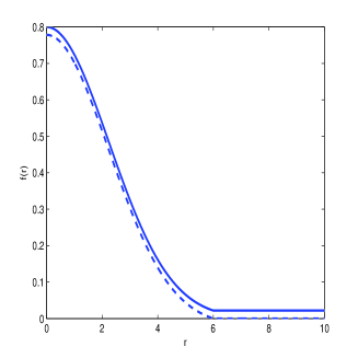
Figure 2: Illustration of $\tilde{f}_{i}$ and $\hat{f}_{i}$ in presence of the limit on sensor range. The solid curve represent the sensor effective function $\tilde{f}_{i}$ and dotted curve is the actual sensor effective function $\hat{f}_{i}(r)=\tilde{f}_{i}(r)+(1-f_{i}(R))$ with $R=6$.

The gradient of (30) with respect to $p_{i}$ can be determined as

$$\frac{\partial(\tilde{\mathcal{H}})}{\partial p_{i}}(\mathcal{P})=2\tilde{M}_{(V_{i}\cap\bar{B}(p_{i},R))}(\tilde{C}_{(V_{i}\cap\bar{B}(p_{i},R)}-p_{i})$$ (31)

We use the control law

$$u_{i}=-k_{prop}(p_{i}-\tilde{C}_{(V_{i}\cap\bar{B}(p_{i},R))})$$ (32)

Remark 5.  It is easy to show, that the gradient (31) and the control law (32) are spatially distributed in the $r$-limited (generalized) Delaunay graph $\mathcal{G}_{LD}$, the Delaunay graph incorporating the sensor range limits.

Theorem 9

The trajectories of the sensors governed by the control law (32), starting from any initial condition $\mathcal{P}(0)$, will asymptotically converge to the critical points of $\tilde{\mathcal{H}}$.

Proof.  The proof is similar to that of the Theorem 4 with $V=-\tilde{\mathcal{H}}(\mathcal{P})$. It can be shown that $V$ is continuously differentiable based on the logic used in Theorem 2.2 in [25]. $\Box$

Thus, agents having limited sensor range can also be used in HSDS and HCDS. However, as noted earlier, Theorems 7 and 8 are not applicable in this situation as the space spanned by the senors is only a subset of the search space $Q$.

IX Implementation issues

Here we discuss some of the theoretical and implementation issues involved in the proposed search strategies namely, heterogeneous sequential deploy and search and heterogeneous combined deploy and search.

A single step of heterogeneous sequential deploy and search strategy involves deploying the agents optimally, and then performing the search task within the respective Voronoi cells. The deployment step can be implemented in continuous time (as given by control law (15)) or in discrete time (as in simulations carried out in this work). When the implementation is in discrete time, in each time step, the agents move toward the corresponding centroids and at the end of the deployment step, that is, when the agents are sufficiently close (as decided by the prescribed tolerance) to the centroids, the search is performed.

IX-A Discrete implementation

We convert the differential equation corresponding to the system dynamics (14) to a difference equation.

$$\frac{\Delta p_{i}}{\Delta t}=u_{i}$$ (33)

where $\Delta t$ is the discrete time step.

Without loss of generality, we let $\Delta t=1$ time unit. Then, (33) will be simplified as,

$${\Delta p_{i}}_{k}={u_{i}}_{k}$$ (34)

and the control law (15) takes the form,

$${u_{i}}_{k}=-k_{prop}({p_{i}}_{k}-\tilde{C}_{V_{ik}})$$ (35)

where $k\in\mathbb{N}$ is the iteration count.

The control input ${u_{i}}_{k}$ is the desired speed of the $i$-th agent at the $k$-th time step. The agent moves with this speed for $\Delta t$ time units. With $\Delta t=1$, ${u_{i}}_{k}$ acts as increment of $p_{i}$ per step. In other words ${u_{i}}_{k}=\Delta p_{i}={p_{i}}_{k+1}-{p_{i}}_{k}$. Thus, if $\Delta t=T$ time units, then the search task takes place after $mT$ time units, where $m$ is a non-zero integer, the number of time steps taken to achieve the optimal deployment. The process is illustrated in Figure 3(a). Search is performed at the end of deployment step and the time instances at which search is performed are marked with ‘*’. The consecutive search task is performed at a time interval of at most $T$ time units. We define the latency, $t_{s}$, of the agents as the maximum time taken to acquire the information, process it, and successfully update the uncertainty density. Finally, $T$ should be chosen to be greater than or equal to $t_{s}$.

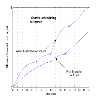
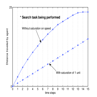
Figure 3: Illustration of the discrete time implementation of (a) heterogeneous sequential deploy and search strategy where deployment takes place according to control law (35) at every time step, and the search task takes place at the end of each deployment step indicated by ‘*’and (b) heterogeneous combined deploy and search strategies where search is performed at every step while the agents move according to the control law (35).

In the heterogeneous combined deploy and search strategy the agents perform search while moving toward corresponding centroids, without waiting till the end of the deployment step. The agents perform search after every $T$ time units as they move toward the respective centroids according to the discrete control law (35). The process is illustrated in Figure 3(b). Search is performed at every time instance as indicated by ‘*’. The plot of distance traveled versus time steps is smoother in case of CDS compared to that of SDS.

IX-B Effect of saturation

The control inputs given by control law (15) or (35) determine the speeds of the agents. In practical implementation, it is likely that there will be a constraint on the maximum speed of agents. Such a limit will appear as a saturation on the control input. In case of the heterogeneous sequential deploy and search strategy, the effect of saturation on control input might lead to slower convergence of the deployment step. During the initial few steps, it is likely that the control input provided by (15) can cross the saturation limit, whereas later, as the agents approach the centroids, the control input naturally reduces (as it is proportional to the distance between the agents and the respective centroids). Thus, effect of saturation is at most a possible increase in the time gap between consecutive search steps as illustrated in Figure 3(a).

In the case of heterogeneous combined deploy and search strategy, whenever the control effort computed by (15) crosses the saturation limit, the actual speed is limited to the saturation value. The time lag between two consecutive search tasks remains fixed at $T$ irrespective of the saturation. But, with saturation, the distance traveled by the agents before performing the next search task reduces (or remains the same if the control input given by (15) is less than the saturation limit). This is illustrated in Figure 3(b). This will probably result in a faster search due to frequent searches.

IX-C Spatial distributedness

Here we discuss the implication of spatial distributedness of the proposed search strategies from a practical point of view. We have seen that both the search strategies are spatially distributed in the generalized Delaunay graph. These results imply that all the agents need to do computations based on only local information, that is, by the knowledge about position of neighboring agents. Also, the agents should have access to the updated uncertainty map within their Voronoi cells. This can be achieved in several ways. One such way is that all the agents communicate with a central information provider. But it is not necessary to have this global information. Each agent can communicate with its Voronoi neighbors ($\mathcal{N}_{\mathcal{G}}(i)$) and obtain the updated uncertainty information in a region $\cup_{\mathcal{N}_{\mathcal{G}}(i)}V_{i}$. As the generalized Voronoi partition $\{V_{i}\}$ depends at least continuously on $\mathcal{P}$, the agent configuration, in an evolving generalized Delaunay graph, the communication within the neighbors is sufficient for each agent to obtain the uncertainty within its new Voronoi cell. The issues related to communication of uncertainty information are not addressed in the paper except to assume that uncertainty information is available to the agents. It is also possible that the agents can estimate the uncertainty map as done in [30].

In practical conditions, the agents can communicate with other agents only when they are within the limits of the sensor range. The generalized Delaunay graph does not allow sensor range limitations to be incorporated. We need to use $r$-limited generalized Delaunay graph or $r$-generalized Delaunay graph (generalized versions of $r$-limited Delaunay graph and $r$-Delaunay [44]) to incorporate the sensor range limitations. It needs to be studied if the proposed search strategies are still spatially distributed on these graphs. In any case, the scenario changes with incorporation of sensor range limitations into the search strategies. The updating of uncertainty density will also be within the sensor range limits (in fact, it is within the region $V_{i}\cap\bar{B}(p_{i},R)$). The centroid that is computed will also be within the new restricted area. For an optimal deployment problem, from the perspective of sensor coverage, it has been observed that the corresponding control law is still spatially distributed (in $r$-limited generalized Delaunay graph) and globally asymptotically stable.

IX-D Synchronization

Synchronization plays an important role in multi-agent systems. Here we discuss this issue for both HSDS and HCDS strategies. In the case of HSDS, theoretically all the agents reach the respective centroid at infinite time. But in a practical implementation, the agents are required to be sufficiently close, where the closeness is suitably defined, to the respective centroids before starting the search operation. It is possible that at any point in time, different agents are at different distances from the corresponding centroid. The agents need to come to a consensus as to when to end the deployment and perform search operation. We have implemented the strategy in a single centralized program using MATLAB. In a practical situation, synchronization can be attained by agents communicating a flag bit indicating if an agent has reached its centroid or not. When all the agents have reached the respective centroid within a tolerance distance, the search can be performed. We also assume that sensing and communication are instantaneous. In our simulation experiments we assume such a communication exists. Since the objective of this work is to evaluate the effectiveness of the search strategies, we make assumptions that simplify implementation without affecting the search effectiveness.

HCDS operates in a synchronous manner by design. If all the agents start at the same instant of time and have synchronized clocks, the search task is performed by every agent after the same interval of time. Given an accurate global clock, synchronization is not a major issue in case of HCDS.

Further in [17] authors provide an asynchronous implementation for coverage control which can be suitably modified for HSDS and HCDS.

X Results and Discussions

A few simulation experiments were carried out to validate the proposed heterogeneous multi-agent search strategies. We used $\beta_{i}=1-k_{i}e^{-\alpha_{i}r_{i}^{2}}$, $i\in\{1,\ldots,N\}$. The search space $Q$ is a square area of size $10\times 10$ in $\mathbb{R}^{2}$. We vary the parameters $k_{i}$s and $\alpha_{i}$s to get different cases.

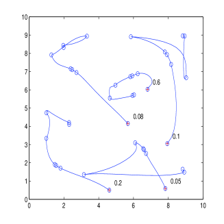
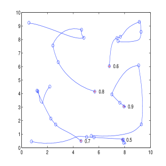
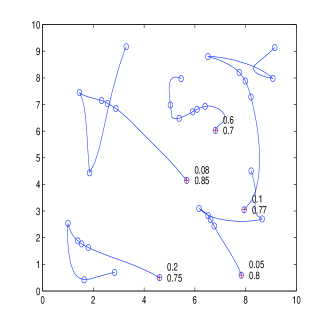
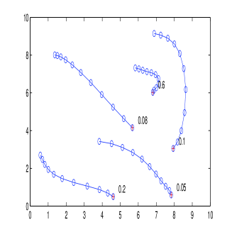
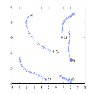
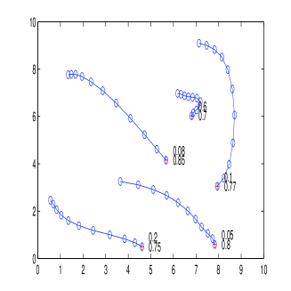
Figure 4: Trajectories for agents with HSDS for $\beta_{i}(r_{i})=1-k_{i}e^{\alpha_{i}r^{2}_{i}}$ with (a) $\alpha_{i}$ varying, (b) $k_{i}$ varying, and (c) both $\alpha_{i}$ and $k_{i}$ varying. Corresponding trajectories with HCDS are shown in (d), (e), and (f). ‘o’ indicate the search instances. The parameters are indicated near the starting location of corresponding agents, which are indicated by ‘+’.

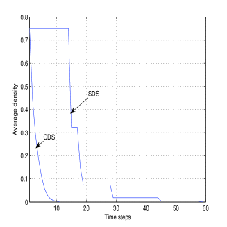
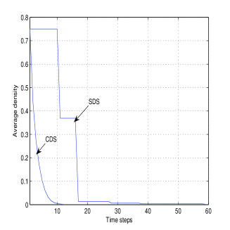
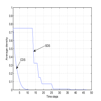
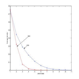
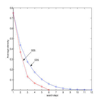
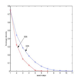
Figure 5: Reduction of uncertainty with HSDS and HCDS with time steps for $\beta_{i}(r_{i})=1-k_{i}e^{\alpha_{i}r^{2}_{i}}$ with (a) $\alpha_{i}$ varying, (b) $k_{i}$ varying, and (c) both $\alpha_{i}$ and $k_{i}$ varying. Corresponding reduction in uncertainty with number of search steps are shown in (d), (e), and (f). ‘o’ indicate the search instances.

Figures 4 and 5 show results of simulation experiments carried out. Figure 4(a) and (d) show the trajectories of the agents for HSDS and HCDS strategies, while Figure 5(a) shows the average uncertainty density history for two strategies with $k_{i}=0.8$ and different $\alpha_{i}$. Figure 5 (d) shows the average uncertainty density with number of searches. The starting location of the agents are marked with ‘+’ and end of each of the deploy steps are marked with ‘o’ along the trajectories for the case of HSDS (Figure 4(a)). It can be observed from Figure 5 (a), that HCDS reduces uncertainty much faster in time compared to HSDS. HSDS takes requires about 20 time steps to reduce the uncertainty below a value of 0.8, while HCDS achieves same reduction in about 6 time steps. This is due to increased frequency of searches in case of HCDS compared to that of HSDS. But Figure 5 (d) reveals that HSDS performs better than HCDS in terms of requiring lesser number of search steps for same amount of uncertainty reduction. In case of HSDS, the agents get optimally deployed before performing the search and hence, compared to HCDS, the uncertainty density is higher in each search step of HSDS.

Figures 4 (b) and (e) show trajectories of agents with $\alpha_{i}=0.1$ and varying $k_{i}$ for HSDS and HCDS, and 5 (b) and (e) show the average uncertainty with number of time steps and number of search steps for both the strategies. Figures 4 (c) and (f), and 5 (c) and (f) show corresponding results with both the parameters $k_{i}$ and $\alpha_{i}$ varying. Values of the varying parameters have been indicated in the figures, near the starting point of each agent which marked with ‘+’.

In all the cases, it can be observed that the trajectories of agents with HCDS strategy are considerably smoother and shorter than those corresponding to the HSDS strategy, nevertheless, both strategies successfully reduce the uncertainty density. The simulation results also indicate that the HCDS strategy performs better even in terms of faster reduction of the average uncertainty density, while HSDS performs better in terms of requiring fewer search instances. It can also be observed that the agents move away from each other covering the search space in a cooperative manner. Figures 5 (a), (b), and (c) illustrate that in HCDS, the search is performed at every time instance, and in HSDS, the search is performed only after optimal deployment of agents.

The simulation results demonstrate that both the proposed heterogeneous search strategies perform well as indicated by the theoretical analysis and that the HCDS strategies performs well in terms of shorter and smoother agent trajectories and faster uncertainty reduction.

When the sensors have heterogeneous capabilities either in terms of effectiveness (indicated by the parameter $k_{i}$) or in terms of the range (indicated by the parameter $\alpha_{i}$), those with higher effectiveness share more load, while the weaker ones may remain inactive (in extreme cases of heterogeneity). The motivation here is to demonstrate the ability to handle heterogeneity in sensors’ capabilities. The sensor parameters are assumed to be given and the problem is of designing a suitable search strategy. It might be interesting to select sensors with required parameters so as to improve the effectiveness of the search strategy. But this design optimization is beyond the scope of this work.

XI Conclusions

We have used a generalization of the Voronoi partition to formulate and solve a heterogeneous multi-agent search problem. The agents having sensors with heterogeneous capabilities were deployed in the search space in an optimal way maximizing per step search effectiveness. The objective function, its critical points, a control law that determines the agent trajectory, its spatial distributedness and convergence properties were discussed. Based on the optimal deployment strategy, two heterogeneous multi-agent search strategies namely heterogeneous sequential deploy and search and heterogeneous combined deploy and search have been proposed and their spatial distributedeness and convergence properties have been studied. Effect of constraints on agents’ speeds and limit on sensor range have been discussed. The simulation experiments demonstrate that the search strategies perform well. The heterogeneous combined deploy and search strategy is seen to perform better in terms of shorter, smoother agent trajectory and faster search.

Analysis of the properties of the generalized Voronoi partition is one of the possible direction for research. Work on effective algorithms for computation related to generalized Voronoi partition will be very useful in effective implementation of the search strategies presented in this paper. Further generalization of the Voronoi partition so as to incorporate anisotropy in the sensors along with the heterogeneity can also be a very useful exercise. With such a generalization, search strategies for multiple agents equipped with heterogeneous and anisotropic sensors can be formulated. It is also interesting to explore new applications of the generalized Voronoi partition.

References

- [1] G.W. Barlow, Hexagonal territories, Animal Behavior, vol. 22, 1974, pp. 876-878.
- [2] B.O. Koopman, Search and Screening, (2nd ed.) Pergamon Press, 1980.
- [3] S.J. Benkoski, M.G. Monticino, and J.R. Weisinger, A survey of the search theory literature, Naval Research Logistics, vol. 38, no. 4, August 1991, pp. 469-494.
- [4] K. Lida, Studies on optimal search plan, Lecture Notes in Statistics, 70, Springer-Verlag, Berling, 1992.
- [5] L.D. Stone, Theory of Optimal Search, Academic Press, New York, 1975.
- [6] D. Enns, D. Bugajski, and S. Pratt, Guidance and control for cooperative search, Proc. of American Control Conference, Anchorage, Alaska, May 2002, pp. 1923-1029.
- [7] S.V. Spires and S.Y. Goldsmith, Exhaustive search with mobile robots along space filling curves, Collective Robotics (Eds. A. Dragoul, M. Tambe, and T. Fukuda), Lecture Notes in Artifcial Intelligence, 1456, Springer-Verlag, 1998 pp. 1-12.
- [8] P. Vincent and I. Rubin, A framework and analysis for cooperative search using UAV swarms, Proc. of ACM Symposium on Applied Computing, Nicosia, Cyprus, 2004, pp 79-86.
- [9] R.W. Beard and T.W. McLain, Multiple UAV cooperative search under collision avoidance and limited range communication constraints, Proc. of IEEE Conference on Decison and Control, Maui, Hawaii, December 2003, pp. 25-30.
- [10] M. Flint, E.F.A. Gaucherand, and M. Polycarpou, Cooperative control for UAVs searching risky environments for targets, Proc. of IEEE Conference on Decision and Control, Maui, Hawaii, December 2003, pp. 3568-3572.
- [11] H.L. Pfister, Cooperative control of autonomous vehicles using fuzzy cognitive maps, Proc. of the AIAA Unmanned unlimited Conference, Workshop, and Exhibit, San Diego, California, September 2003, AIAA-2003-6506.
- [12] M. Polycarpou, Y. Yang and K. Passino, A cooperative search framework for distributed agents, Proc. of IEEE International Symposium on Intelligent Control, Mexico, September 2001, pp. 1-6.
- [13] Y. Yang, A.A. Minai, and M.M. Polycarpou, Analysis of opportunistic method for cooperative search by mobile agents, Proc. of IEEE Conference on Decision and Control, Las Vegas, Nevada, December 2002 pp 576-577.
- [14] Y. Yang, A.A. Minai, and M.M. Polycarpou, Decentralized cooperative search in UAVs using opportunistic learning, Proc. of AIAA Guidance, Navigation and Control Conference, Montery, California, August 2002, AIAA pp 2002-4590.
- [15] D.G. Rajnarayan and D. Ghose, Multiple agent team theoretic decision making for searching unknown environments, Proc. of IEEE Conference on Decision and Control, Maui, Hawaii, December 2003, pp. 2543-2548.
- [16] R.F. Dell, J.N. Eagel, G.H.A. Martins, and A.G. Santos, Using multiple searchers in constrained-path, moving-target search problems, Naval Research Logistics, vol. 43, pp. 463-480, 1996.
- [17] P.B. Sujit and D. Ghose, Multiple UAV search using agent based negotiation scheme, Proc. of American Control Conference, June 8-10, 2005. Portland, OR, USA, pp. 2995-3000.
- [18] Y. Jin, A.A. Minai, M.M. Polycarpou, Cooperative real-time search and task allocation in UAV teams, Proceedings of the 42nd IEEE Conference on Decision and Control, Maui, Hawaii, USA, December 2003, pp. 7-12.
- [19] G. Voronoi. Nouvelles applications des param tres continus la th orie des formes quadratiques. Journal f r die Reine und Angewandte Mathematik, vol. 133, 1907. pp. 97-178.
- [20] G.L. Dirichlet. ber die Reduktion der positiven quadratischen Formen mit drei unbestimmten ganzen Zahlen. Journal f r die Reine und Angewandte Mathematik, vol. 40, 1850, pp. 209-227.
- [21] F. Aurenhammer, Voronoi Diagrams - A survey of a fundamental geometric data structure, ACM Computing Surveys, vol. 23, no. 3, 1991, pp. 345-405.
- [22] E.B. Kosmatopoulos and M.A. Christodoulou, Convergence properties of a class of learning vector quantization algorithms, IEEE Transactions on Image Processing, vol. 5, no. 2, February, 1996, pp. 361-368.
- [23] P.A. Arbel aez and L.D. Cohen, Generalized Voronoi tessellations for vector-valued image segmentation, Proceedings 2nd IEEE Workshop on Variational, Geometric and Level Set Methods in Computer Vision (VLSM’03), Nice, France, September 2003.
- [24] J. Cortes, S. Martinez, T. Karata, and F. Bullo, Coverage control for mobile sensing networks, IEEE Transactions on Robotics and Automation, vol. 20, no. 2, 2004, pp. 243-255.
- [25] J. Cortes, S. Martinez, and F. Bullo, Spatially-distributed coverage optimization and control with limited-range interactions, ESAIM: Control, Optimization and Calculus of Variations, vol. 11, no. 4, 2005, pp. 691-719.
- [26] B. Delaunay, Sur la sph re vide, Izvestia Akademii Nauk SSSR, Otdelenie Matematicheskikh i Estestvennykh Nauk, vol. 7, 1934. pp.793-800.
- [27] Z. Drezner, Facility location: A survey of applications and methods, New York, NY: Springer, 1995.
- [28] A. Okabe, B. Boots, K. Sugihara, and S. Chiu, Spatial Tessellations: Concepts and Applications of Voronoi Diagrams, Wiley & Sons, Chichester, UK, 2000.
- [29] Q. Du, V. Faber, M. Gunzburger, Centroidal Voronoi tessellations: applications and algorithms, SIAM Review, vol. 41, no. 4, 1999, pp. 637-676.
- [30] M. Schwager, J. McLurkin and D. Rus, Distributed coverage control with sensory feedback for newtorked robots, Proc. of Robotics: Science and Systems, Philadelphia, PA, Aug , 2006.
- [31] L.C.A. Pimenta, V. Kumar, R.C. Mesquita, and A.S. Pereira, Sensing and coverage for a network of heterogeneous robots, in Proc. of 47th IEEE Conference on Decision and Control, Cancun, Mexico, December, 2008, pp. 3947-3952.
- [32] M. Ma and Y. Yang, Adaptive triangular deployment algorithm for unatended mobile sesnor networks, IEEE Trans. on Computers, vol. 56, no. 7, July, 2007, pp. 946-948.
- [33] K.R. Guruprasad and D. Ghose, Multi-Agent Search using Voronoi partitions, Proceedings of the International Conference on Advances in Control and Optimization of Dynamical Systems (ACODS), February, 2007, pp. 380-383.
- [34] K.R. Guruprasad and D. Ghose, Deploy and search strategy for multi-agent systems using Voronoi partitions, Proceedings of 4th international Symposium on Voronoi Diagrams in Science and Engineering (ISVD 2007), University of Glamorgan, Wales, UK, July 9-11, 2007, pp. 91-100.
- [35] K.R. Guruprasad, Multi-agent search using Voronoi partition, Ph.D Thesis, Indian Institute of Science, Bangalore, INDIA, December, 2008.
- [36] K.R. Guruprasad and D. Ghose, Multi-agent search using sensors with heterogeneous capabilities, to appear in Proceedings of the 7th International Conference on Autonomous Agents and Multiagent Systems (AAMAS 2008), May 12-16, 2008, Estoril, Portugal. pp. 1397-1400.
- [37] J.P. LaSalle, Some extensions of Liapunov’s second method, IRE Transactions on Circuit Theory, CT-7(4), December, 1960, pp. 520-527
- [38] E.A. Barbashin and N.N. Krasovski, Ob ustoichivosti dvizheniya v tzelom, Dokl. Akad. Nauk., USSR, vol. 86, no. 3, 1952, pp. 453-456.
- [39] H.J. Marquez, Nonlinear Control Systems - Analysis and Design, John Wiley & Sons, Inc., 2003.
- [40] P.K. Kundu and I.M. Cohen, Fluid mechanics (2nd ed.), Academic Press, 2002.
- [41] H. Edelsbrunner and R. Seidel, Voronoi diagrams and arrangements, Discrete Comput. Geom., vol 1, 1986, pp. 25-44.
- [42] S.G. Krantz and H.R. Parks, A Primer of Real Analytic Functions (2nd edn.), Birkhäuser Advanced Texts, Basler Lehbücher, 2002.
- [43] J-C Fort and Pages̀ G. On the a.s. convergence of the Kohonen algorithm with a general neighborhood function, The Annals of Applied Probability, vol.5, no. 4, 1995, pp. 1177-1216.
- [44] R. Diestel, Graph Theory. (2nd edn.), Graduate Texts in Mathematics, New York, Springer-Verlag, 2000.