The dispersion of growth of matter perturbations in $f(R)$ gravity

Abstract

We study the growth of matter density perturbations $\delta_{m}$ for a number of viable $f(R)$ gravity models that satisfy both cosmological and local gravity constraints, where the Lagrangian density $f$ is a function of the Ricci scalar $R$. If the parameter $m\equiv Rf_{,RR}/f_{,R}$ today is larger than the order of $10^{-6}$, linear perturbations relevant to the matter power spectrum evolve with a growth rate $s\equiv{\rm d}\ln\delta_{m}/{\rm d}\ln a$ ($a$ is the scale factor) that is larger than in the $\Lambda$CDM model. We find the window in the free parameter space of our models for which spatial dispersion of the growth index $\gamma_{0}\equiv\gamma(z=0)$ ($z$ is the redshift) appears in the range of values $0.40\lesssim\gamma_{0}\lesssim 0.55$, as well as the region in parameter space for which there is essentially no dispersion and $\gamma_{0}$ converges to values around $0.40\lesssim\gamma_{0}\lesssim 0.43$. These latter values are much lower than in the $\Lambda$CDM model. We show that these unusual dispersed or converged spectra are present in most of the viable $f(R)$ models with $m(z=0)$ larger than the order of $10^{-6}$. These properties will be essential in the quest for $f(R)$ modified gravity models using future high-precision observations and they confirm the possibility to distinguish clearly most of these models from the $\Lambda$CDM model.

I Introduction

The origin of dark energy (DE) responsible for the cosmic acceleration today has been a lasting mystery review . Although a host of independent observational data have supported the existence of DE over the past ten years, no strong evidence was found yet implying that dynamical DE models are better than a cosmological constant $\Lambda$. A first step towards understanding the origin of DE would be to detect some clear deviation from the $\Lambda$CDM model observationally and experimentally.

Models such as quintessence quin based on minimally coupled scalar fields provide a dynamical equation of state of DE different from $w_{\rm DE}=-1$. Still it is difficult to distinguish these models from the $\Lambda$CDM model in current observations pertaining to the cosmic expansion history only (such as the supernovae Ia observations). Even if we consider the evolution of matter perturbations $\delta_{m}$ in these models, the growth rate of $\delta_{m}$ is similar to that in the $\Lambda$CDM model. Hence one cannot generally expect large differences with the $\Lambda$CDM model at both the background and the perturbation levels.

There is another class of DE models in which gravity is modified with respect to General Relativity (GR). The simplest one would be the so-called $f(R)$ gravity where the Lagrangian density $f$ is a function of the Ricci scalar $R$ fRearly . The basic idea is that gravity is modified on cosmological scales when $R$ is of the order of $H_{0}^{2}$ ($H_{0}$ is the Hubble parameter today), while Newtonian gravity is recovered in the region of high density ($R\gg H_{0}^{2}$). A number of viable $f(R)$ models have been constructed in this spirit AGPT ; Li ; AT08 ; Hu ; Star ; Appleby ; Tsuji ; N007 ; Linder . Since the law of gravity is modified in $f(R)$ models, we can in principle expect large differences with the $\Lambda$CDM model in cosmological observations obserpapers ; lensing and in laboratory tests lgcpapers ; Navarro ; CT compared to quintessence models.

From a cosmological point of view viable $f(R)$ models are similar to the $\Lambda$CDM model during the radiation and deep matter eras (“GR regime”), but important observable deviations from the $\Lambda$CDM model appear at late times as the model evolves towards what we call here the “scalar-tensor regime” [see below after Eq. (13)]. A useful quantity that characterizes this deviation is $m=Rf_{,RR}/f_{,R}$ AGPT , where $f_{,R}\equiv\partial f/\partial R$ and $f_{,RR}\equiv\partial^{2}f/\partial R^{2}$. In order to satisfy local gravity constraints we require that $m$ is much smaller than 1 for $R\gg H_{0}^{2}$, e.g., $m(R)\lesssim 10^{-15}$ for $R\approx 10^{5}H_{0}^{2}$ AT08 ; CT ; Tavakol . Meanwhile, in order to see appreciable deviation from the $\Lambda$CDM model at the background level of cosmological evolution, the parameter $m$ needs to grow to the of order at least 0.01-0.1 today. The models proposed in Refs. Hu ; Star ; Appleby ; Tsuji ; Linder are constructed to realize this fast transition of $m$. Actually as we will see, the quantity $m$ is related to the (critical) scale $\sim M^{-1}=\left(3m/R\right)^{1/2}$ below which modifications of gravity are felt by the matter perturbations. For increasing $m$ and for decreasing $R$, this critical scale gets larger.

The modified evolution of the matter density perturbations $\delta_{m}$ provides an important tool to distinguish $f(R)$ models, and generally modified gravity DE models, from DE models inside GR and in particular from the $\Lambda$CDM model obserpapers . In fact the effective gravitational “constant” $G_{\rm eff}$ which appears in the source term driving the evolution of matter perturbations can change significantly relative to the gravitational constant $G$ in the usual GR regime, i.e. $G_{\rm eff}\simeq(4/3)G$ (the “scalar-tensor” regime). Then the evolution of perturbations during the matter era changes from $\delta_{m}\propto t^{2/3}$ to $\delta_{m}\propto t^{(\sqrt{33}-1)/6}$, where $t$ is the cosmic time Star ; Tsuji .

A useful way to describe the perturbations is to write the growth function $s={\rm d}\ln\delta_{m}/{\rm d}\ln a$ as $s=(\Omega_{m})^{\gamma}$, where $\Omega_{m}$ is the density parameter of non-relativistic matter. As well-known one has $\gamma_{0}\equiv\gamma(z=0)\simeq 0.55$ Wang ; Lindergamma in the $\Lambda$CDM model. It was emphasized that while $\gamma$ is quasi-constant in standard (non-interacting) DE models inside GR with $\gamma_{0}\simeq 0.55$, this needs not be the case in modified gravity models, in particular large slopes can appear PG08 (see Refs. gammapapers for more related works). For the model proposed by Starobinsky Star it was found in Ref. GMP09 that the present value of the growth index $\gamma_{0}$ can be as small as $\gamma_{0}=$0.40-0.43 while large slopes are obtained. This allows to clearly discriminate this model from $\Lambda$CDM. An additional important point is whether $\gamma_{0}$ can exhibit some dispersion (scale dependence) for viable $f(R)$ DE models.

The redshift at which the transition of perturbations occurs depends on the comoving wavenumber $k$. It is then expected that the resulting matter power spectrum has a scale dependence for viable $f(R)$ models. In this paper we shall study the dependence of the growth index $\gamma$ on scales relevant to the linear regime of the matter power spectrum. We consider most of viable $f(R)$ models proposed in literature to understand general properties of the dispersion of perturbations. This analysis will be important to distinguish between the $f(R)$ models and the $\Lambda$CDM model in future observations of galaxy clustering and weak lensing.

II Cosmology in $f(R)$ gravity

We start with the action

$$S=\frac{1}{2\kappa^{2}}\int{\rm d}^{4}x\sqrt{-g}f(R)+S_{m}(g_{\mu\nu},\Psi_{m})\,,$$ (1)

where $\kappa^{2}=8\pi G$ ($G$ is bare gravitational constant), and $S_{m}$ is a matter action that depends on the metric $g_{\mu\nu}$ and matter fields $\Psi_{m}$. Since we are interested in the cosmological evolution at the late epoch, we only consider a perfect fluid of non-relativistic matter with an energy density $\rho_{m}$. In the following we use the unit $\kappa^{2}=1$, but we restore the gravitational constant $G$ when the discussion becomes transparent.

In the flat Friedmann-Lemaître-Robertson-Walker (FLRW) spacetime with scale factor $a(t)$, the variation of the action (1) leads to the following equations

$$3FH^{2} = \rho_{m}+(FR-f)/2-3H\dot{F},$$ (2)

$$-2F\dot{H} = \rho_{m}+\ddot{F}-H\dot{F},$$ (3)

where $F\equiv\partial f/\partial R$, $H\equiv\dot{a}/a$, and a dot represents a derivative with respect to the cosmic time $t$. The Ricci scalar $R$ is expressed by the Hubble parameter $H$ as $R=6(2H^{2}+\dot{H})$. In order to study the cosmological dynamics in $f(R)$ gravity, it is convenient to introduce the following variables

$$x_{1}=-\frac{\dot{F}}{HF}\,,\quad x_{2}=-\frac{f}{6FH^{2}}\,,\quad x_{3}=\frac{R}{6H^{2}}\,,$$ (4)

together with the matter density parameter

$$\tilde{\Omega}_{m}\equiv\frac{\rho_{m}}{3FH^{2}}=1-x_{1}-x_{2}-x_{3}\,.$$ (5)

We then obtain the following dynamical equations AGPT

$$x_{1}^{\prime} = -1-x_{3}-3x_{2}+x_{1}^{2}-x_{1}x_{3}\,,$$ (6)

$$x_{2}^{\prime} = \frac{x_{1}x_{3}}{m(r)}-x_{2}(2x_{3}-4-x_{1})\,,$$ (7)

$$x_{3}^{\prime} = -\frac{x_{1}x_{3}}{m(r)}-2x_{3}(x_{3}-2)\,,$$ (8)

where a prime represents a derivative with respect to $N=\ln a$, and

$$m(r)\equiv\frac{Rf_{,RR}}{f_{,R}}\,,\quad r\equiv-\frac{Rf_{,R}}{f}=\frac{x_{3}}{x_{2}}\,.$$ (9)

One has $m=0$ for the $\Lambda$CDM model ($f(R)=R-2\Lambda$), so that the quantity $m$ characterizes the deviation from the $\Lambda$CDM model. Since $m$ is a function of $r=x_{3}/x_{2}$, the above dynamical equations are closed. For given functional forms of $f(R)$, the background cosmological dynamics is known by solving Eqs. (6)-(8) with Eq. (9). The matter point $P_{m}$ and the de Sitter point $P_{\rm dS}$ correspond to AGPT

• $P_{m}$: $(x_{1},x_{2},x_{3})=\left(\frac{3m}{1+m},-\frac{1+4m}{2(1+m)^{2}},\frac{1+4m}{2(1+m)}\right)$,
         $\tilde{\Omega}_{m}=1-\frac{m(7+10m)}{2(1+m)^{2}}$,    $w_{\rm eff}=-\frac{m}{1+m}$ .

• $P_{\rm dS}$: $(x_{1},x_{2},x_{3})=(0,-1,2)$,
         $\tilde{\Omega}_{m}=0$,    $w_{\rm eff}=-1$ .

We require that $m\approx 0$ to realize the matter era with $\tilde{\Omega}_{m}\approx 1$ and $w_{\rm eff}\approx 0$. From the definition of $r$ in Eq. (9) we have $r=-m-1$ for $P_{m}$, so that the matter point corresponds to $(r,m)\approx(-1,0)$ in the $(r,m)$ plane. Note that the radiation point also exists around $(r,m)\approx(-1,0)$ AGPT . The de Sitter point $P_{\rm dS}$ correspond to the line $r=-2$.

Let us next consider linear perturbations about the flat FLRW background. In the so-called comoving gauge Hwang where the velocity perturbation of non-relativistic matter vanishes, the matter perturbation $\delta_{m}=\delta\rho_{m}/\rho_{m}$ and the perturbation $\delta F$ obey the following equations in the Fourier space Hwang ; Tsuji

$$\ddot{\delta}_{m}+\left(2H+\frac{\dot{F}}{2F}\right)\dot{\delta}_{m}-\frac{\rho_{m}}{2F}\delta_{m}$$

$$=\frac{1}{2F}\left[\left(-6H^{2}+\frac{k^{2}}{a^{2}}\right)\delta F+3H\dot{\delta F}+3\ddot{\delta F}\right],$$ (10)

$$\ddot{\delta F}+3H\dot{\delta F}+\left(\frac{k^{2}}{a^{2}}+\frac{f_{,R}}{3f_{,RR}}-\frac{R}{3}\right)\delta F$$

$$=\frac{1}{3}\rho_{m}\delta_{m}+\dot{F}\dot{\delta}_{m}\,,$$ (11)

where $k$ is a comoving wavenumber. We also define

$$M^{2}\equiv\frac{f_{,R}}{3f_{,RR}}=\frac{R}{3m}\,,$$ (12)

which corresponds to the mass squared of the scalar-field degree of freedom, the scalaron introduced in S80 , in the region $M^{2}\gg R$. As we will see later, the quantity $m$ remains smaller than the order of $0.1$ in the cosmic expansion history and the condition $M^{2}\gg R$ is largely satisfied at high redshifts.

For cosmologically viable models, the variation of $F$ is small ($|\dot{F}|\ll HF$) so that the terms including $\dot{F}$ can be neglected in Eqs. (10) and (11). If we neglect the oscillating mode of $\delta F$ relative to the mode induced by matter perturbations $\delta_{m}$, it follows that $\delta F\simeq\rho_{m}\delta_{m}/[3(k^{2}/a^{2}+M^{2})]$ from Eq. (11). For the modes deep inside the Hubble radius ($k^{2}/a^{2}\gg H^{2}$) the dominant term in the square bracket of Eq. (10) is $(k^{2}/a^{2})\delta F$. We then obtain the following approximate equation for matter perturbations Tsuji07 ; Tavakol

$$\ddot{\delta}_{m}+2H\dot{\delta}_{m}-4\pi G_{\rm eff}\rho_{m}\delta_{m}\simeq 0\,,$$ (13)

where

$$G_{\rm eff} \equiv \frac{G}{F}\frac{4k^{2}/a^{2}+3M^{2}}{3(k^{2}/a^{2}+M^{2})}$$ (14)

$$= \frac{G}{F}\leavevmode\nobreak\ \left[1+\frac{1}{3}\frac{k^{2}/(a^{2}M^{2})}{1+k^{2}/(a^{2}M^{2})}\right]\,.$$ (15)

Here we have restored bare gravitational constant $G$. An equation of a similar type was found for scalar-tensor DE models BEPS00 with an essentially massless dilaton field. The quantity $G_{\rm eff}$ encodes the modification of gravity in the weak-field regime due to the presence of the dilaton in the case of scalar-tensor DE models, and of the scalaron in our $f(R)$ models. An essential difference is that the scalaron mass $M$ in the region of high density can be large, inducing a finite range $\sim M^{-1}$ for the (Yukawa type) “fifth-force”.

Under the linear expansion of the Ricci scalar $R$ in the weak gravity background of a spherically symmetric spacetime, the effective Newtonian gravitational constant is given by lgcpapers ; Navarro

$$G_{\rm eff}^{(\rm N)}=\frac{G}{F}\left(1+\frac{1}{3}\leavevmode\nobreak\ e^{-Mr}\right)\,,$$ (16)

where $r$ is the distance from the center of symmetry.

Poisson’s equation in Fourier space with $G$ replaced by $G_{\rm eff}^{(\rm N)}$ as given in Eq. (16) corresponds to the gravitational potential in real space (between two unit masses) $V(r)=-G_{\rm eff}^{(\rm N)}/r$. It corresponds to the modification of gravity in the weak-field regime that is felt by the cosmological perturbations.

For the validity of the linear expansion of $R$ the mass $M$ needs to be light such that $Mr_{c}\ll 1$, where $r_{c}$ is the radius of a spherically symmetric body. For small scales satisfying $r\ll M^{-1}$, the fifth-force reaches its maximal value and the modification of gravity reduces to a shift of the gravitational constant $G\to 4G/(3F)$. This is the regime we have called here the “scalar-tensor” regime. Cosmologically the corresponding shift in the scalar-tensor DE models mentioned above depends on time and occurs on all scales. Note that in the massive regime $Mr_{c}\gg 1$ the result (16) is no longer valid. It is exactly in this regime where the chameleon mechanism KW begins to be at work so that the effective gravitational constant becomes very close to $G$ to satisfy local gravity constraints Navarro ; Hu ; AT08 (as we will see in the next section).

In the region $M^{2}\gg k^{2}/a^{2}$ the cosmological effective gravitational constant (15) reduces to the form $G_{\rm eff}\simeq G/F$. Then the evolution of $\delta_{m}$ during the matter era is given by $\delta_{m}\propto t^{2/3}$ (note that $F\simeq 1$ because the deviation parameter $m$ is much smaller than 1). In the region $M^{2}\ll k^{2}/a^{2}$ we have $G_{\rm eff}\simeq 4G/(3F)$, so that the matter perturbation evolves as $\delta_{m}\propto t^{(\sqrt{33}-1)/6}$ during the matter era Star .

The perturbation equation (13) has been derived for sub-horizon modes under the neglect of the oscillating mode (such as the term $\ddot{\delta F}$). For cosmologically viable models, the solutions obtained by solving Eq. (13) agrees well with full numerical solutions Tavakol ; Cruz ; Motohashi . In our numerical simulations, however, we shall solve the full perturbation equations (10) and (11) together with the background equations (6)-(8), without relying on the approximate equation (13). For the numerical integration it is convenient to rewrite Eqs. (10) and (11) in the following forms Tsuji

$$\delta_{m}^{\prime\prime}+\left(x_{3}-\frac{1}{2}x_{1}\right)\delta_{m}^{\prime}-\frac{3}{2}(1-x_{1}-x_{2}-x_{3})\delta_{m}$$

$$=\frac{1}{2}\biggl{[}\left\{\frac{k^{2}}{x_{4}^{2}}-6+3x_{1}^{2}-3x_{1}^{\prime}-3x_{1}(x_{3}-1)\right\}\delta\tilde{F}$$

$$\leavevmode\nobreak\ \leavevmode\nobreak\ \leavevmode\nobreak\ \leavevmode\nobreak\ \leavevmode\nobreak\ \leavevmode\nobreak\ \leavevmode\nobreak\ +3(-2x_{1}+x_{3}-1)\delta\tilde{F}^{\prime}+3\delta\tilde{F}^{\prime\prime}\biggr{]}\,,$$ (17)

$$\delta\tilde{F}^{\prime\prime}+(1-2x_{1}+x_{3})\delta\tilde{F}^{\prime}$$

$$+\left[\frac{k^{2}}{x_{4}^{2}}-2x_{3}+\frac{2x_{3}}{m}-x_{1}(x_{3}+1)-x_{1}^{\prime}+x_{1}^{2}\right]\delta\tilde{F}$$

$$=(1-x_{1}-x_{2}-x_{3})\delta_{m}-x_{1}\delta_{m}^{\prime}\,,$$ (18)

where $\delta\tilde{F}\equiv\delta F/F$, and the new variable $x_{4}\equiv aH$ satisfies

$$x_{4}^{\prime}=(x_{3}-1)x_{4}\,.$$ (19)

The growth index $\gamma$ of matter perturbations is defined as

$$s\equiv(\Omega_{m})^{\gamma}\,,$$ (20)

where $s\equiv{\rm d}\ln\delta_{m}/{\rm d}\ln a=\delta_{m}^{\prime}/\delta_{m}$ and $\Omega_{m}$ is given by

$$\Omega_{m}\equiv\frac{\rho_{m}}{3H^{2}}=F\tilde{\Omega}_{m}\,.$$ (21)

This choice of $\Omega_{m}$ comes from rewriting Eq. (2) in the form $3H^{2}=\rho_{m}+\rho_{\rm DE}$, where $\rho_{\rm DE}\equiv(FR-f)/2-3H\dot{F}+3H^{2}(1-F)$ Star ; GMP09 . For viable $f(R)$ models the quantity $F$ approaches 1 in the asymptotic past because they are similar to the $\Lambda$CDM model (as we will see in the next section). Defining $\rho_{\rm DE}$ as well as $\Omega_{m}$ in the above way, the Friedmann equations recast in their usual General Relativistic form for dust-like matter and DE.

III Viable $f(R)$ models

Let us briefly review viable $f(R)$ models that can satisfy both cosmological and local gravity constraints. We focus on the models in which cosmological solutions have a late-time de Sitter attractor at $R=R_{1}\leavevmode\nobreak\ (>0)$. For the viability of $f(R)$ models the following conditions need to be satisfied.

• (i) $f_{,R}>0$ for $R\geq R_{1}\leavevmode\nobreak\ (>0)$. This is required to avoid anti-gravity.

• (ii) $f_{,RR}>0$ for $R\geq R_{1}$. This is required for the stability of cosmological perturbations obserpapers , for the presence of a matter era APT , and for consistency with local gravity tests lgcpapers .

• (ii) $f(R)\to R-2\Lambda$ for $R\gg R_{0}$, where $R_{0}$ is the Ricci scalar today. This is required for consistency with local gravity tests lgcpapers and for the presence of radiation and matter eras AGPT .

• (iv) $0<m(r=-2)<1$. This is required for the stability of the late-time de Sitter point Sch ; Fara ; AGPT .

The conditions (i) and (ii) mean that $m=Rf_{,RR}/f_{,R}>0$ for $R\geq R_{1}$. The trajectories starting from $(r,m)\approx(-1,+0)$ to the de Sitter point on the line $r=-2$, $0<m<1$ are acceptable. In other words, the deviation parameter $m$ is initially small ($0<m\ll 1$) so that the model is close to the $\Lambda$CDM model during the radiation and deep matter eras. The deviation from the $\Lambda$CDM model can be important at the late epoch. Depending on the models of $f(R)$ gravity, the parameter $m$ can grow as large as to the order of 0.1 today.

We also require the condition $0<m\ll 1$ in the region $R\gg R_{0}$ for consistency with local gravity constraints. In this case the mass squared $M^{2}$ in Eq. (12) becomes large in the region of high density to avoid the propagation of the fifth force. It is then possible for $f(R)$ models to satisfy local gravity constraints under the chameleon mechanism KW . We introduce a new metric variable $\tilde{g}_{\mu\nu}$ and a scalar field $\phi$, as $\tilde{g}_{\mu\nu}=\psi g_{\mu\nu}$ and $\phi=\sqrt{3/2}\,\ln\psi$, where $\psi=F(R)$. The action in the Einstein frame is then given by Maeda

$$S = \int{\rm d}^{4}x\sqrt{-\tilde{g}}\left[\tilde{R}/2-(\tilde{\nabla}\phi)^{2}/2-V(\phi)\right]$$ (22)

$$+S_{m}(\tilde{g}_{\mu\nu}e^{2Q\phi},\Psi_{m})\,,$$

where

$$Q=-\frac{1}{\sqrt{6}}\,,\quad V=\frac{R(\psi)\psi-f}{2\psi^{2}}\,.$$ (23)

The scalar field degree of freedom $\phi$ has a constant coupling $Q$ with non-relativistic matter in the Einstein frame.

In a spherically symmetric spacetime of the Minkowski background the field $\phi$ obeys the following equation in the Einstein frame

$$\frac{{\rm d}^{2}\phi}{{\rm d}\tilde{r}^{2}}+\frac{2}{\tilde{r}}\frac{{\rm d}\phi}{{\rm d}\tilde{r}}=\frac{{\rm d}V_{\rm eff}}{{\rm d}\phi}\,,$$ (24)

where $\tilde{r}$ is the distance from the center of symmetry and

$$V_{\rm eff}(\phi)=V(\phi)+e^{Q\phi}\rho^{*}\,.$$ (25)

Here $\rho^{*}=e^{3Q\phi}\rho_{m}$ is a conserved matter density in the Einstein frame KW . For $f(R)$ models ($Q=-1/\sqrt{6}$) the effective potential $V_{\rm eff}(\phi)$ possesses a minimum for $V_{,\phi}(\phi)>0$. For a spherically symmetric body with constant densities $\rho_{A}$ and $\rho_{B}$ inside and outside the star, the effective potential has two minima at the field values $\phi_{A}$ and $\phi_{B}$ satisfying the conditions $V_{{\rm eff},\phi}(\phi_{A})=0$ and $V_{{\rm eff},\phi}(\phi_{B})=0$, respectively, with mass squared $m_{A}^{2}\equiv V_{{\rm eff},\phi\phi}(\phi_{A})$ and $m_{B}^{2}\equiv V_{{\rm eff},\phi\phi}(\phi_{B})$. We define the so-called thin shell parameter KW

$$\epsilon_{\rm th}\equiv\frac{\phi_{B}-\phi_{A}}{6Q\Phi_{c}}\,,$$ (26)

where $\Phi_{c}$ is the gravitational potential at the surface of the body ($\tilde{r}=\tilde{r}_{c}$). If the field $\phi$ is sufficiently heavy such that $m_{A}\tilde{r}_{c}\gg 1$ and if the body has a thin-shell in the region $\tilde{r}_{1}<\tilde{r}<\tilde{r}_{c}$ with $\Delta\tilde{r}_{c}\equiv\tilde{r}_{c}-\tilde{r}_{1}\ll\tilde{r}_{c}$, the thin-shell parameter is given by $\epsilon_{\rm th}\simeq\Delta\tilde{r}_{c}/\tilde{r}_{c}+1/(m_{A}\tilde{r}_{c})\ll 1$ Tamaki . The effective coupling between non-relativistic matter and the field $\phi$ is $Q_{\rm eff}\simeq 3Q\epsilon_{\rm th}$, whose strength can be much smaller than 1 for $\epsilon_{\rm th}\ll 1$.

The tightest bound on $\epsilon_{\rm th}$ comes from the solar system test of the violation of equivalence principle for the accelerations of Earth and Moon toward Sun KW . This constraint is given by Tsuji08

$$\epsilon_{\rm th,\oplus}<8.8\times 10^{-7}/|Q|\,,$$ (27)

where $\epsilon_{\rm th,\oplus}$ is the thin-shell parameter for Earth. Since the gravitational potential for Earth is $\Phi_{c,\oplus}=7.0\times 10^{-10}$, the condition (27) translates into

$$|\phi_{B,\oplus}|<3.7\times 10^{-15}\,,$$ (28)

where we have used $|\phi_{B,\oplus}|\gg|\phi_{A,\oplus}|$. For cosmologically viable $f(R)$ models, $|\phi_{B,\oplus}|$ is roughly the same order as the deviation parameter $m(R_{B})$ at the Ricci scalar $R_{B}$ AT08 (as we will see below). Hence the condition $m(R_{B})\lesssim 10^{-15}$ needs to be satisfied in the region around Earth (in which $R_{B}\gg R_{0}$). Cosmologically this means that the parameter $m$ is very much smaller than 1 in radiation and deep matter eras.

We consider $f(R)$ models which can be consistent with both cosmological and local gravity constraints. They can all be written in the form:

$$f(R)=R-\lambda R_{c}\,f_{1}(x)\,,\qquad x\equiv R/R_{c}\,,$$ (29)

where $R_{c}\leavevmode\nobreak\ (>0)$ defines a characteristic value of the Ricci scalar $R$ and $\lambda$ is some positive free parameter.

We will study the following models:

• (A) $f_{1}(x)=x^{p}$  ($0<p<1$) ,

• (B) $f_{1}(x)=x^{2n}/(x^{2n}+1)$  ($n>0$) ,

• (C) $f_{1}(x)=1-(1+x^{2})^{-n}$  ($n>0$) ,

• (D) $f_{1}(x)=1-e^{-x}$ ,

• (E) $f_{1}(x)=\tanh(x)$ .

For $\lambda$ of the order of unity, $R_{c}$ roughly corresponds to the scale of the cosmological Ricci scalar $R_{0}$ today.

The model (A) is characterized by $m=p(r+1)/r$, which behaves as $m\simeq p(-r-1)$ during radiation and deep matter eras ($r\simeq-1$) AGPT . In the regime $R\gg R_{c}$ we have $\phi\simeq-(\sqrt{6}/2)m/(1-p)$ with $m\simeq\lambda p(1-p)(R/R_{c})^{p-1}$. In order to satisfy the condition (28) the parameter $p$ is constrained to be very small: $p<3\times 10^{-10}$ CT .

In the regime $R\gg R_{c}$ the models (B) and (C), proposed by Hu and Sawicki Hu and Starobinsky Star respectively, behave as

$$f(R)\simeq R-\lambda R_{c}\left[1-(R/R_{c})^{-2n}\right]\,,$$ (30)

which corresponds to

$$m(r)=C(-r-1)^{2n+1}\,,\quad C=2n(2n+1)/\lambda^{2n}\,,$$ (31)

with the field value $\phi\simeq-(\sqrt{6}/2)m/(2n+1)$. Because of the presence of the power $2n+1$ in Eq. (31), the condition (28) can be satisfied even for $n$ and $\lambda$ of the order of unity. In fact the models (B) and (C) are consistent with the constraint (28) for $n>0.9$ CT . In these models the deviation parameter $m$ can grow to the order of 0.1 today.

The models (D) and (E), proposed by Linder Linder and Tsujikawa Tsuji respectively, have vanishingly small $m$ in the region $R\gg R_{c}$, but $m$ can grow to ${\cal O}(0.1)$ once $R$ decreases to the order of $R_{c}$ (see Ref. Appleby for a similar model). In the model (D) one has $m\simeq\lambda(R/R_{c})e^{-R/R_{c}}$ for $R\gg R_{c}$, where $R/R_{c}\simeq\log(-\sqrt{2/3}\phi/\lambda)$. The field value $\phi_{B}$ can be derived by solving $V_{{\rm eff},\phi}(\phi_{B})=0$ with $\rho^{*}\simeq\rho_{B}$, which gives $R\simeq\rho_{B}$. We then find that $\phi_{B}\simeq-\sqrt{3/2}\lambda e^{-\rho_{B}/R_{c}}$. Since $\lambda R_{c}$ is of the order of the cosmological density $\rho_{c}^{(0)}\simeq 10^{-29}$ g/cm³ today, we have $\phi_{B}\approx-\lambda e^{-10^{5}\lambda}$ by using the dark matter/baryonic density $\rho_{B}\simeq 10^{-24}$ g/cm³ in our galaxy. As we will see later the existence of a stable de Sitter point demands $\lambda>1$, under which the constraint (28) is well satisfied. The model (E) also has a similar property. Thus the models (D) and (E) are consistent with local gravity constraints for $\lambda$ required for viable cosmology.

IV Growth indices of matter perturbations

In this section we study the growth of matter perturbations for the viable $f(R)$ models (A)-(E). We are interested in the wavenumbers $k$ relevant to the galaxy power spectrum Percival :

$$0.01\leavevmode\nobreak\ h\,{\rm Mpc}^{-1}\lesssim k\lesssim 0.2\leavevmode\nobreak\ h\,{\rm Mpc}^{-1}\,,$$ (32)

where $h=0.72\pm 0.08$ corresponds to the uncertainty of the Hubble parameter today HST . The scales (32) are in the linear regime of perturbations. For $k=0.2\leavevmode\nobreak\ h\leavevmode\nobreak\ {\rm Mpc}^{-1}$, non-linear effects are still small so that results in the linear regime can be related to observations. Non-linear effects increase as we go to smaller scales. On the other hand we should remember that observations on the large scale around $k\sim 0.01\leavevmode\nobreak\ h\,{\rm Mpc}^{-1}$ are not so accurate but will be improved in the future.

We recall that the transition from the “GR regime” to the “scalar-tensor regime” occurs at $M^{2}=k^{2}/a^{2}$. Using Eq (12) this translates into

$$m\approx(aH/k)^{2}\,.$$ (33)

This expresses in terms of the quantity $m$ the fact that cosmic scales smaller than $\sim M^{-1}$ will be affected by modifications of gravity. For viable $f(R)$ models we have presented in the previous section, the deviation parameter $m$ increases from the matter era to the accelerated epoch. For larger $k$ (i.e. for smaller scales) the transition occurs earlier. The upper bound of the wavenumber in Eq. (32) corresponds to $k\simeq 600a_{0}H_{0}$, where the subscript “0” represents present quantities. We are interested in the case where the transition to the scalar-tensor regime occurred by the present epoch (the redshift $z=0$). This then gives the following condition

$$m(z=0)\gtrsim 3\times 10^{-6}\,.$$ (34)

If $m(z=0)\lesssim 3\times 10^{-6}$ then the linear perturbations have been always in the GR regime in the past, so that the models are not distinguished from the $\Lambda$CDM model. We caution that the bound (34) is relaxed for non-linear perturbations with $k\gtrsim 0.2\,h$ Mpc^-1, but the linear analysis is not valid in such cases.

In our numerical simulations we identify the present epoch to be $\Omega_{m}^{(0)}=0.28$.

IV.1 Model (A)

Let us first consider the model (A). In this model the deviation parameter $m=p(r+1)/r$ corresponds to $m=p/2$ at the de Sitter point ($r=-2$), which means that $m(z=0)$ is of the order of $p$. Hence the condition (34) for the occurrence of the transition to the scalar-tensor regime corresponds to

$$p\gtrsim 6\times 10^{-6}\,.$$ (35)

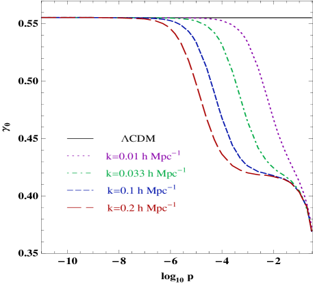
Figure 1: The growth indices $\gamma_{0}$ today versus the parameter $p$ in the model (A) for four different values of $k$. Under the local gravity bound $p<3\times 10^{-10}$, the deviation of $\gamma_{0}$ from that in the $\Lambda$CDM model ($\gamma_{0}\simeq 0.55$) cannot be seen for these wavenumbers.

In Fig. 1 we plot the growth indices $\gamma_{0}$ of matter perturbations today for four different wavenumbers $k$. When $p\gtrsim 6\times 10^{-6}$ the deviation from the value $\gamma_{0}\simeq 0.55$ of the $\Lambda$CDM model can be clearly seen for the modes $k\gtrsim 0.2\,h\leavevmode\nobreak\ {\rm Mpc}^{-1}$. The dispersion of $\gamma_{0}$ with respect to the wavenumbers $k$ is especially significant for $10^{-5}<p<10^{-2}$, whereas $\gamma_{0}$ converges to a value around $0.4$ for $p\gtrsim 10^{-1}$.

We recall that local gravity constraints give the bound $p<3\times 10^{-10}$, which is not compatible with the condition (35). Under this bound the growth indices are very close to the $\Lambda$CDM value $\gamma_{0}\simeq 0.55$ for the wavenumbers (32). Hence the model (A) cannot be distinguished from the $\Lambda$CDM model as long as local gravity constraints are respected.

IV.2 Models (B) and (C)

We shall proceed to the models (B) and (C). In the region $R\gg R_{c}$ these models can be described by the $m(r)$ curve given in Eq. (31). In the deep matter era ($r\approx-1$) the deviation parameter $m$ gets smaller for increasing $n$ because of the larger power-law index $2n+1$ in Eq. (31). For increasing $\lambda$ we also have smaller $m$.

In the model (B) the stability of the late-time de Sitter point requires that Tsuji07

$$2x_{d}^{4n}-(2n-1)(2n+4)x_{d}^{2n}+(2n-1)(2n-2)\geq 0,$$ (36)

where $x_{d}=R_{1}/R_{c}$.

The parameter

$$\lambda=\frac{(1+x_{d}^{2n})^{2}}{x_{d}^{2n-1}(2+2x_{d}^{2n}-2n)}\,,$$ (37)

has a lower bound determined by the condition (36). When $n=1$, for example, one has $x_{d}\geq\sqrt{3}$ and $\lambda\geq 8\sqrt{3}/9$.

Similarly the model (C) satisfies

$$(1+x_{d}^{2})^{n+2}>1+(n+2)x_{d}^{2}+(n+1)(2n+1)x_{d}^{4},$$ (38)

with

$$\lambda=\frac{x_{d}(1+x_{d}^{2})^{n+1}}{2[(1+x_{d}^{2})^{n+1}-1-(n+1)x_{d}^{2}]}\,.$$ (39)

When $n=1$ we have $x_{d}\geq\sqrt{3}$ and $\lambda\geq 8\sqrt{3}/9$, which is the same as in the model (B). For general $n$, however, the bounds on $\lambda$ in the model (C) are not identical to those in the model (B). The minimum values of $\lambda$ are of the order of unity in both models.

At the de Sitter point the model (31) gives $m(r=-2)=C=2n(2n+1)/\lambda^{2n}$, so that $m(z=0)$ can be as large as ${\cal O}(1)$ for $n,\lambda$ of the order of unity. Numerically we find that the deviation parameter $m(z=0)$ in the models (B) and (C) is typically smaller than that in the model (31), but still $m(z=0)$ can be of the order of 0.1. The deviation parameter $m$ needs to be very much smaller than 1 in the region of high density ($R\gg R_{c}$) for consistency with local gravity constraints.

If the transition characterized by the condition (33) occurs during the deep matter era ($z\gg 1$), one can estimate the critical redshift $z_{c}$ at the transition point. We use the asymptotic forms $m\simeq C(-r-1)^{2n+1}$ and $r\simeq-1-\lambda R_{c}/R$ as well as the approximate relations $H^{2}\simeq H_{0}^{2}\Omega_{m}^{(0)}(1+z)^{3}$ and $R\simeq 3H^{2}$. The present value of $\rho_{\rm DE}$ may be approximated as $\rho_{\rm DE}^{(0)}\approx\lambda R_{c}/2$. Hence we have that $\lambda R_{c}\approx 6H_{0}^{2}\Omega_{\rm DE}^{(0)}$, where $\Omega_{\rm DE}^{(0)}$ is the DE density parameter today. Then the condition (33) translates into the critical redshift

$$z_{c}=\left[\left(\frac{k}{a_{0}H_{0}}\right)^{2}\frac{2n(2n+1)}{\lambda^{2n}}\frac{(2\Omega_{\rm DE}^{(0)})^{2n+1}}{{\Omega_{m}^{(0)}}^{2(n+1)}}\right]^{\frac{1}{6n+4}}-1.$$ (40)

For $n=1$, $\lambda=3$, $k=300a_{0}H_{0}$, and $\Omega_{m}^{(0)}=0.28$ in the model (C) the numerical value for the critical redshift is $z_{c}=4.5$, which shows good agreement with the analytical value estimated by Eq. (40). We caution, however, that Eq. (40) begins to lose its accuracy for $z_{c}$ close to 1.

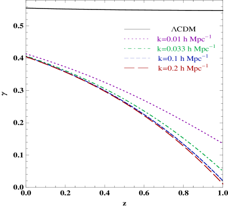
Figure 2: The evolution of $\gamma$ versus the redshift $z$ in the model (B) with $n=1$ and $\lambda=1.55$ for four different values of $k$. In this case the dispersion of $\gamma$ with respect to $k$ is very small. It is nearly absent for scales $k\geq 0.033\leavevmode\nobreak\ h\leavevmode\nobreak\ {\rm Mpc}^{-1}$, so these scales have reached today the asymptotic regime $k\gg aM$.

We recall that local gravity constraints give the bound $n>0.9$ for both the models (B) and (C). Meanwhile the conditions (36)-(39) provide lower bounds on $\lambda$ for each $n$ ($\lambda>1.54$ for $n=1$ in both models). In Fig. 2 we plot the evolution of the growth indices $\gamma$ in the model (B) with $n=1$ and $\lambda=1.55$ for a number of different wavenumbers. We find a degeneracy of the present value of $\gamma$ around $\gamma_{0}\simeq 0.41$ independent of the scales of our interest. In this case the transition redshift corresponds to $z_{c}=5.2$ and $z_{c}=2.7$ for the modes $k=0.1\,h\,{\rm Mpc}^{-1}$ and $k=0.01\,h\,{\rm Mpc}^{-1}$, respectively. At the present epoch these modes are in the “scalar-tensor” regime with similar growth indices.

Equation (40) shows that $z_{c}$ gets smaller for increasing $n$. In Fig. 3 we show the present values of $\gamma$ versus $n$ in the model (B) with $\lambda=1.55$ for four different wavenumbers. We find that $\gamma_{0}$ has a scale dependence in the region $0.42\lesssim\gamma_{0}\lesssim 0.55$ for $2\lesssim n\lesssim 7$, while $\gamma_{0}$ is degenerate around $0.41$ for $n$ close to 1. This reflects the fact that, for larger $n$, the transition redshift $z_{c}$ gets smaller. The growth indices are strongly dispersed if the mode $k=0.2\,h\,{\rm Mpc}^{-1}$ crossed the transition point at $z_{c}>{\cal O}(1)$ and the mode $k=0.01\,h\,{\rm Mpc}^{-1}$ has marginally entered (or has not entered) the scalar-tensor regime by today. Since $z_{c}$ decreases for increasing $\lambda$ from Eq. (40), it is expected that the scale dependence of $\gamma_{0}$ can appear for larger $\lambda$ than in the case shown in Fig. 3 (for fixed $n$). In fact this behavior is clearly seen in the numerical simulation of Fig. 4, which shows that in the model (B) with $n=1$ the dispersion of $\gamma_{0}$ occurs for $0.5\lesssim\log_{10}\,\lambda\lesssim 2.5$. If $\lambda\gtrsim 10^{3}$, $\gamma_{0}$ converges to the $\Lambda$CDM value $\simeq 0.55$ because the modes (32) have not entered the scalar-tensor regime by today.

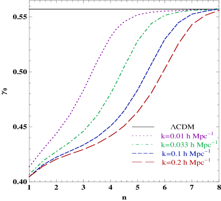
Figure 3: The growth indices $\gamma_{0}$ today versus $n$ in the model (B) with $\lambda=1.55$ for four different values of $k$. The dispersion of $\gamma_{0}$ occurs in the region $0.42\lesssim\gamma_{0}\lesssim 0.55$ for $2\lesssim n\lesssim 7$.

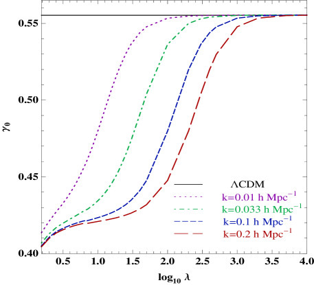
Figure 4: The growth indices $\gamma_{0}$ today versus $\lambda$ in the model (B) with $n=1$ for four different values of $k$. The dispersion of $\gamma_{0}$ appears for $0.5\lesssim\log_{10}\lambda\lesssim 2.5$.

We have also carried out numerical simulations for the model (C) and found that the evolution of $\gamma$ is very similar to that in the model (B) for the same values of $n$ and $\lambda$. Let us consider the parameter regions of $(n,\lambda)$ for the models (B) and (C) in which the dispersion of $\gamma_{0}$ occurs for the wavenumbers (32). We can divide the $(n,\lambda)$ plane in three regions:

• (i) All modes have the values of $\gamma_{0}$ close to the $\Lambda$CDM value: $\gamma_{0}=0.55$, i.e. $0.53\lesssim\gamma_{0}\lesssim 0.55$.

• (ii) All modes have the values of $\gamma_{0}$ close to the value in the range $0.40\lesssim\gamma_{0}\lesssim 0.43$.

• (iii) The values of $\gamma_{0}$ are dispersed in the range $0.40\lesssim\gamma_{0}\lesssim 0.55$.

We recall that the first case arises when all scales under consideration are close to the asymptotic regime for scales larger today than the range of the “fifth-force”. The second case corresponds to the opposite situation. In the third case some of the scales belong to the intermediate regime Gannouji09 . To find out accurately when the asymptotic regimes are reached, and what are the values of $\gamma_{0}$ in the intermediate regime, one has to resort to numerical calculations.

The region (i) is characterized by the opposite of the inequality (34), i.e. $m(z=0)\lesssim 3\times 10^{-6}$. This corresponds to the case in which $n$ and $\lambda$ take large values so that $m$ is suppressed. The border between (i) and (iii) is determined by the condition $m(z=0)\approx 3\times 10^{-6}$. The region (ii) corresponds to small values of $n$ and $\lambda$, as in the numerical simulation of Fig. 2. In this case the mode $k=0.01\,h\,{\rm Mpc}^{-1}$ at least entered the scalar-tensor regime for $z_{c}>{\cal O}(1)$.

The regions (i), (ii), (iii) can be found by solving perturbation equations numerically. Note that we also have the local gravity constraint $n>0.9$ as well as the conditions (36) and (38) with (37) and (39) coming from the stability of the late-time de Sitter point. In Fig. 5 we illustrate the regions (i), (ii), (iii) for the models (B) and (C), which are quite similar in both models. The parameter space for $n\lesssim 3$ and $\lambda={\cal O}(1)$ is dominated by either the region (ii) or the region (iii). These unusual converged or dispersed spectra can be useful to distinguish the $f(R)$ gravity from the $\Lambda$CDM model.

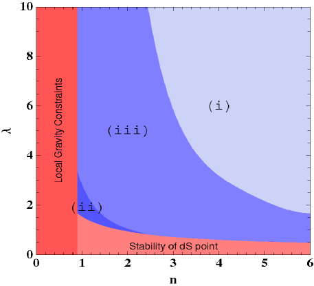
Figure 5: The regions (i), (ii) and (iii) for the model (B) (top) and for the model (C) (bottom). The three regions in the model (B) are similar to those in the model (C).

IV.3 Models (D) and (E)

The deviation parameter $m$ in the model (D) is given by

$$m=\frac{\lambda xe^{-x}}{1-\lambda e^{-x}}\,.$$ (41)

In the region $R\gg R_{c}$ we have that $m\simeq\lambda xe^{-x}$, which means that $m$ rapidly decreases as we go back to the past. In the asymptotic past the model (E) has a similar dependence $m\simeq 8\lambda xe^{-2x}$. In both models the parameter $r$ behaves as $r\simeq-1-\lambda/x$ for $R\gg R_{c}$.

For the model (D) the Ricci scalar at the de Sitter point ($x_{d}=R_{1}/R_{c}$) is determined by $\lambda$, as

$$\lambda=\frac{x_{d}}{2-(2+x_{d})e^{-x_{d}}}\,.$$ (42)

From Eqs. (41) and (42) we find that the stability condition $m(R_{1})<1$ is satisfied for $x_{d}>0$. It then follows from Eq. (42) that $\lambda$ is bounded to be

$$\lambda>1\,.$$ (43)

If the crossing $M^{2}=k^{2}/a^{2}$ occurs during the matter era, the transition redshift $z_{c}$ for the model (D) can be estimated as

$$\frac{2\Omega_{\rm DE}^{(0)}}{\lambda^{2}(1+z_{c})^{2}}\exp\left[\frac{\Omega_{m}^{(0)}\lambda(1+z_{c})^{3}}{2\Omega_{\rm DE}^{(0)}}\right]=\left(\frac{k}{a_{0}H_{0}}\right)^{2}\,.$$ (44)

The redshift $z_{c}$ gets larger for increasing $k$ and for decreasing $\lambda$. If $k=300a_{0}H_{0}$ and $\lambda=1.1$ we have $z_{c}=3.0$ from the estimation (44). This is slightly different from the numerical value $z_{c}=2.7$ because the transition point is close to the onset of the cosmic acceleration.

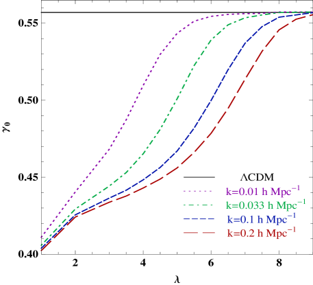
Figure 6: The growth indices $\gamma_{0}$ today versus $\lambda$ in the model (D) for four different values of $k$. We note that the transition is much faster in terms of $\lambda$ than in model (B) shown in Fig. 4.

In Fig. 6 we plot the growth indices $\gamma_{0}$ today versus $\lambda$ for four different wavenumbers. If $\lambda$ is close to 1 then $0.40<\gamma_{0}<0.42$, so that the dispersion of $\gamma_{0}$ is weak. The dispersion begins to appear for $\lambda>2$. This is associated with the fact that the transition redshift gets smaller for increasing $\lambda$. If the condition $m(z=0)\lesssim 3\times 10^{-6}$ is satisfied, the transition does not occur by today so that $\gamma_{0}$ is close to the $\Lambda$CDM value $0.55$ for the modes (32). Numerically the present value of $x$ is found to be $x_{0}\approx 2.2\lambda$. Plugging this into Eq. (41), we find that the condition $m(z=0)\lesssim 3\times 10^{-6}$ translates into $\lambda\gtrsim 8$. This shows that the dispersion of $\gamma_{0}$ in the range $0.40\lesssim\gamma_{0}\lesssim 0.55$ occurs for $2\lesssim\lambda\lesssim 8$. This can be confirmed in the numerical simulation of Fig. 6. For $\lambda\gtrsim 8$, $\gamma_{0}$ converges to the $\Lambda$CDM value $\simeq 0.55$.

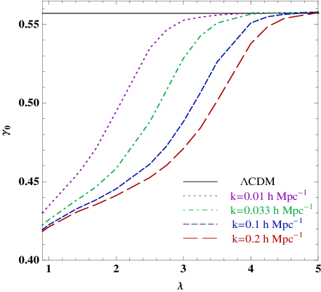
Figure 7: The growth indices $\gamma_{0}$ today versus $\lambda$ in the model (E) for four different values of $k$. It is seen that the transition for this model is slightly more rapid in terms of $\lambda$ than in model (D) shown in Fig. 6.

For the model (E) we have

$$m=\frac{2\lambda x\tanh(x)[1-\tanh^{2}(x)]}{1-\lambda[1-\tanh^{2}(x)]}\,.$$ (45)

The de Sitter point is determined by the relation

$$\lambda=\frac{x_{d}\cosh^{2}(x_{d})}{2\sinh(x_{d})\cosh(x_{d})-x_{d}}\,.$$ (46)

From the stability of the de Sitter point we require that Tsuji07

$$\lambda>0.905\,,\quad x_{d}>0.920\,.$$ (47)

As in the model (D) the numerical value of $x_{0}$ is about $x_{0}\approx 2.2\lambda$. It then follows from Eq. (45) that the condition $m(z=0)\lesssim 3\times 10^{-6}$ corresponds to $\lambda\gtrsim 4$, in which case $\gamma_{0}$ is degenerate to $\gamma_{0}\simeq 0.55$ for the modes (32). In Fig. 7 the dispersion of $\gamma_{0}$ can be seen for $\lambda\lesssim 4$. When $\lambda$ is close to the minimum value $0.905$, the growth indices are almost degenerate in the range $0.42\lesssim\gamma_{0}\lesssim 0.43$.

V Conclusions

In this paper we have studied the dispersion of the growth index $\gamma$ of matter perturbations in $f(R)$ gravity models. We focused on a number of viable $f(R)$ dark energy models proposed in the literature that can satisfy cosmological and local gravity constraints. While these models are close to the $\Lambda$CDM model in the asymptotic past, a deviation from the $\Lambda$CDM model appears at late times. A useful quantity that characterizes this deviation is given by $m=Rf_{,RR}/f_{,R}$. This quantity needs to be very much smaller than 1 during the deep matter era for consistency with local gravity constraints, but a growth of $m$ to the present value of the order of 0.1 can be allowed depending on the $f(R)$ models.

The transition of matter perturbations from the GR regime to the scalar-tensor regime occurs at the epoch characterized by the condition $m\approx(aH/k)^{2}$. For the wavenumbers $k$ relevant for the observable range of the linear matter power spectrum ($0.01\,h\,{\rm Mpc}^{-1}\lesssim k\lesssim 0.2\,h\,{\rm Mpc}^{-1}$), we require that $m(z=0)\gtrsim 3\times 10^{-6}$ for the occurrence of such a transition by today. For the model (A) this requirement is not compatible with local gravity constraints and hence this model cannot be distinguished from the $\Lambda$CDM model.

The models (B) and (C) allow for a rapid growth of $m$ from the region $R\gg H_{0}^{2}$ [with $m(R)\lesssim 10^{-15}$] to the region $R\simeq H_{0}^{2}$ [with $m(R)={\cal O}(0.1)$]. When $n<3$ and $\lambda={\cal O}(1)$ we find two distinct regions widely spread in the $(n,\lambda)$ plane: the region (ii) in which the present growth indices $\gamma_{0}$ almost converge to the values around $0.40\lesssim\gamma_{0}\lesssim 0.43$ and the region (iii) in which $\gamma_{0}$ are dispersed around $0.40\lesssim\gamma_{0}\lesssim 0.55$. In the first region there is essentially no spatial dispersion of $\gamma_{0}$, in contrast to the second region. These results are summarized in Fig. 5 for the models (B) and (C).

The models (D) and (E) give rise to an even faster evolution of $m$ compared to the models (B) and (C). The evolution of $\gamma$ depends on the single parameter $\lambda$. For the models (D) and (E) the dispersion of $\gamma_{0}$ in the region $0.40\lesssim\gamma_{0}\lesssim 0.55$ is found for $2\lesssim\lambda\lesssim 8$ and $1.5\lesssim\lambda\lesssim 4$, respectively. The growth indices converge to values around $0.40\lesssim\gamma_{0}\lesssim 0.43$ for $1<\lambda\lesssim 2$ [model (D)] and for $0.905<\lambda\lesssim 1.5$ [model (E)].

We have thus shown that the dispersed or converged growth indices with $\gamma_{0}$ smaller than 0.55 are present in viable $f(R)$ models with $m(z=0)\gtrsim 3\times 10^{-6}$. If future observations detect such unusually small values of $\gamma_{0}$, this can be a smoking gun for $f(R)$ models. The presence of some dispersion in future observations could be an additional evidence for some of our $f(R)$ models. We also note that our analysis can be extended to scalar-tensor models with couplings $Q$ of the order of 1 between dark energy and non-relativistic matter in the Einstein frame Tsuji08 ; Gannouji09 . It will be of interest to investigate the growth of matter perturbations and the resulting dispersion of $\gamma$ in such theories.

References

- (1) V. Sahni and A. A. Starobinsky, Int. J. Mod. Phys. D 9, 373 (2000); S. M. Carroll, Living Rev. Rel. 4, 1 (2001); T. Padmanabhan, Phys. Rept. 380, 235 (2003); P. J. E. Peebles and B. Ratra, Rev. Mod. Phys. 75, 559 (2003); E. J. Copeland, M. Sami and S. Tsujikawa, Int. J. Mod. Phys. D 15, 1753 (2006); V. Sahni, A. A. Starobinsky, Int. J. Mod. Phys. D15, 2105 (2006); T. P. Sotiriou and V. Faraoni, arXiv:0805.1726 [gr-qc]; R. Durrer and R. Maartens, arXiv:0811.4132 [astro-ph].
- (2) Y. Fujii, Phys. Rev. D 26, 2580 (1982); L. H. Ford, Phys. Rev. D 35, 2339 (1987); C. Wetterich, Nucl. Phys B. 302, 668 (1988); B. Ratra and J. Peebles, Phys. Rev D 37, 321 (1988); T. Chiba, N. Sugiyama and T. Nakamura, Mon. Not. Roy. Astron. Soc. 289, L5 (1997); R. R. Caldwell, R. Dave and P. J. Steinhardt, Phys. Rev. Lett. 80, 1582 (1998).
- (3) S. Capozziello, Int. J. Mod. Phys. D 11, 483, (2002); S. Capozziello, V. F. Cardone, S. Carloni and A. Troisi, Int. J. Mod. Phys. D, 12, 1969 (2003); S. M. Carroll, V. Duvvuri, M. Trodden and M. S. Turner, Phys. Rev. D 70, 043528 (2004); S. Nojiri and S. D. Odintsov, Phys. Rev. D 68, 123512 (2003).
- (4) L. Amendola, R. Gannouji, D. Polarski and S. Tsujikawa, Phys. Rev. D 75, 083504 (2007).
- (5) L. Amendola and S. Tsujikawa, Phys. Lett. B 660, 125 (2008).
- (6) B. Li and J. D. Barrow, Phys. Rev. D 75, 084010 (2007).
- (7) W. Hu and I. Sawicki, Phys. Rev. D 76, 064004 (2007).
- (8) A. A. Starobinsky, JETP Lett. 86, 157 (2007).
- (9) S. A. Appleby and R. A. Battye, Phys. Lett. B 654, 7 (2007).
- (10) S. Tsujikawa, Phys. Rev. D 77, 023507 (2008).
- (11) S. Nojiri and S. D. Odintsov, Phys. Lett. B 657, 238 (2007); G. Cognola et al., Phys. Rev. D 77, 046009 (2008).
- (12) E. V. Linder, arXiv:0905.2962 [astro-ph.CO].
- (13) S. M. Carroll, I. Sawicki, A. Silvestri and M. Trodden, New J. Phys. 8, 323 (2006); T. Faulkner, M. Tegmark, E. F. Bunn and Y. Mao, Phys. Rev. D 76, 063505 (2007); Y. S. Song, W. Hu and I. Sawicki, Phys. Rev. D 75, 044004 (2007); R. Bean, D. Bernat, L. Pogosian, A. Silvestri and M. Trodden, Phys. Rev. D 75, 064020 (2007); Y. S. Song, H. Peiris and W. Hu, Phys. Rev. D 76, 063517 (2007); Y. S. Song, H. Peiris and W. Hu, Phys. Rev. D 76, 063517 (2007); L. Pogosian and A. Silvestri, Phys. Rev. D 77, 023503 (2008); T. Tatekawa and S. Tsujikawa, JCAP 0809, 009 (2008); H. Oyaizu, M. Lima and W. Hu, Phys. Rev. D 78, 123524 (2008); K. Koyama, A. Taruya and T. Hiramatsu, arXiv:0902.0618 [astro-ph.CO].
- (14) M. Ishak, A. Upadhye and D. N. Spergel, Phys. Rev. D 74, 043513 (2006); A. F. Heavens, T. D. Kitching and L. Verde, Mon. Not. Roy. Astron. Soc. 380, 1029 (2007); L. Amendola, M. Kunz and D. Sapone, JCAP 0804, 013 (2008); S. Tsujikawa and T. Tatekawa, Phys. Lett. B 665, 325 (2008); F. Schmidt, Phys. Rev. D 78, 043002 (2008); Y. S. Song and O. Dore, arXiv:0812.0002 [astro-ph].
- (15) G. J. Olmo, Phys. Rev. D 72, 083505 (2005); A. L. Erickcek, T. L. Smith and M. Kamionkowski, Phys. Rev. D 74, 121501 (2006); V. Faraoni, Phys. Rev. D 74, 023529 (2006); T. Chiba, T. L. Smith and A. L. Erickcek, Phys. Rev. D 75, 124014 (2007); P. Brax, C. van de Bruck, A. C. Davis and D. J. Shaw, Phys. Rev. D 78, 104021 (2008); I. Thongkool, M. Sami, R. Gannouji and S. Jhingan, arXiv:0906.2460 [hep-th].
- (16) I. Navarro and K. Van Acoleyen, JCAP 0702, 022 (2007).
- (17) S. Capozziello and S. Tsujikawa, Phys. Rev. D 77, 107501 (2008).
- (18) S. Tsujikawa, K. Uddin and R. Tavakol, Phys. Rev. D 77, 043007 (2008).
- (19) L. M. Wang and P. J. Steinhardt, Astrophys. J. 508, 483 (1998).
- (20) E. V. Linder, Phys. Rev. D 72, 043529 (2005); D. Huterer and E. V. Linder, Phys. Rev. D 75, 023519 (2007).
- (21) D. Polarski and R. Gannouji, Phys. Lett. B 660, 439 (2008); R. Gannouji and D. Polarski, JCAP 0805, 018 (2008).
- (22) E. Bertschinger, Astrophys. J. 648, 797 (2006); K Yamamoto et al., Phys. Rev. D 76, 023504 (2007); C. Di Porto and L. Amendola, Phys. Rev. D 77, 083508 (2008); S. Nesseris and L. Perivolaropoulos, Phys. Rev. D 77, 023504 (2008); G. Ballesteros and A. Riotto, Phys. Lett. B 668, 171 (2008); Y. Gong, Phys. Rev. D 78, 123010 (2008); H. Wei and S. N. Zhang, Phys. Rev. D 78, 023011 (2008); H. Wei, Phys. Lett. B 664, 1 (2008); S. A. Thomas, F. B. Abdalla and J. Weller, arXiv:0810.4863 [astro-ph]; U. Alam, V. Sahni and A. A. Starobinsky, arXiv:0812.2846 [astro-ph]. E. V. Linder, Phys. Rev. D 79, 063519 (2009); P. Wu, H. Yu and X. Fu, JCAP 0906, 019 (2009); J. H. He, B. Wang and Y. P. Jing, JCAP 0907, 030 (2009); Y. Gong, M. Ishak and A. Wang, arXiv:0903.0001 [astro-ph.CO]; J. B. Dent, S. Dutta and L. Perivolaropoulos, arXiv:0903.5296 [astro-ph.CO]; S. Lee and K. W. Ng, arXiv:0905.1522 [astro-ph.CO]; M. Ishak and J. Dossett, arXiv:0905.2470 [astro-ph.CO].
- (23) R. Gannouji, B. Moraes and D. Polarski, JCAP 0902, 034 (2009).
- (24) J. c. Hwang and H. Noh, Phys. Rev. D 71, 063536 (2005).
- (25) A. A. Starobinsky, Phys. Lett. B 91, 99 (1980).
- (26) S. Tsujikawa, Phys. Rev. D 76, 023514 (2007).
- (27) B. Boisseau, G. Esposito-Farese, D. Polarski and A. A. Starobinsky, Phys. Rev. Lett. 85, 2236 (2000).
- (28) J. Khoury and A. Weltman, Phys. Rev. Lett. 93, 171104 (2004); Phys. Rev. D 69, 044026 (2004).
- (29) A. de la Cruz-Dombriz, A. Dobado and A. L. Maroto, Phys. Rev. D 77, 123515 (2008).
- (30) H. Motohashi, A. A. Starobinsky and J. Yokoyama, arXiv:0905.0730 [astro-ph.CO].
- (31) L. Amendola, D. Polarski and S. Tsujikawa, Phys. Rev. Lett. 98, 131302 (2007); Int. J. Mod. Phys. D 16, 1555 (2007).
- (32) V. Muller, H. J. Schmidt and A. A. Starobinsky, Phys. Lett. B 202, 198 (1988).
- (33) V. Faraoni, Phys. Rev. D 72, 124005 (2005).
- (34) K. i. Maeda, Phys. Rev. D 39, 3159 (1989).
- (35) T. Tamaki and S. Tsujikawa, Phys. Rev. D 78, 084028 (2008).
- (36) S. Tsujikawa, K. Uddin, S. Mizuno, R. Tavakol and J. Yokoyama, Phys. Rev. D 77, 103009 (2008).
- (37) W. J. Percival et al., Astrophys. J. 657, 645 (2007).
- (38) W. L. Freedman et al. [HST Collaboration], Astrophys. J. 553, 47 (2001).
- (39) R. Gannouji, B. Moraes and D. Polarski, arXiv:0907.0393 [astro-ph.CO].