Light-induced polarization effects in atoms with partially resolved hyperfine structure and applications to absorption, fluorescence, and nonlinear magneto-optical rotation

Abstract

The creation and detection of atomic polarization is examined theoretically, through the study of basic optical-pumping mechanisms and absorption and fluorescence measurements, and the dependence of these processes on the size of ground- and excited-state hyperfine splittings is determined. The consequences of this dependence are studied in more detail for the case of nonlinear magneto-optical rotation in the Faraday geometry (an effect requiring the creation and detection of rank-two polarization in the ground state) with alkali atoms. Analytic formulas for the optical rotation signal under various experimental conditions are presented.

I Introduction

Since the pioneering work of Alfred Kastler and Jean Brossel in the 1950s Kastler (1967), atomic polarization created by the interaction of light with atoms have been an exciting topic of research, providing new methods for laser spectroscopy and delivering new technologies for practical applications, such as narrow-band optical filters Yeh (1982).

Atomic polarization, created in a medium by polarized light, can modify the optical response of the medium, affecting the light field. For example, the absorption of light of a particular polarization by atoms in a polarized state can be reduced (electromagnetically induced transparency Fleischhauer et al. (2005)) or increased (electromagnetically induced absorption Lezama et al. (1999)) compared to that for an unpolarized state. Coherent population trapping Nasyrov et al. (2006) is a closely related phenomenon, the study of which led to the discovery of an interesting effect that is also a powerful tool for the manipulation of atomic states: coherent population transfer between atomic states, known as STIRAP (stimulated Raman adiabatic passage) Bergmann et al. (1998). “Lasing without inversion” Kocharovskaya and Khanin Ya (1988); Scully et al. (1989) is another related effect.

Additional effects are encountered when atoms interact with coherent light in the presence of a magnetic field Budker et al. (2002); Alexandrov et al. (2005). (Reference Budker and Rochester (2004) discusses a relationship between these effects and electromagnetically induced absorption.) These magneto-optical effects—especially those involving magnetic-field-induced evolution of long-lived ground-state polarization—can be used to perform sensitive magnetometery Budker and Romalis (2007). (These effects are also often referred to as “coherence effects”, although this is something of a misnomer, as in some cases the effects can be described using a basis in which there are no ground-state coherences Kanorsky et al. (1993).)

The atomic polarization responsible for specific effects, such as nonlinear magneto-optical rotation (NMOR), can be described in terms of the polarization moments (PM) in the multipole expansion of the density matrix Omont (1977); Auzinsh and Ferber (1995). The lowest-rank multipole moments correspond to population, described by a rank $\kappa=0$ tensor, orientation, described by a rank $\kappa=1$ tensor, and alignment, described by a rank $\kappa=2$ tensor. It is these three lowest-rank multipole moments that can directly affect light absorption and laser-induced fluorescence Dyakonov (1965); Auzinsh and Ferber (1995), and thus can be created and detected through single-photon interactions. An atomic state with total angular momentum $F$ can support multipole moments with rank up to $\kappa=2F$ Omont (1977); Auzinsh and Ferber (1995); multi-photon interactions and multipole transitions higher than dipole allow the higher-order moments to be created and detected. Magneto-optical techniques can be used to selectively address individual high-rank multipoles Auzin’sh and Ferber (1984); Yashchuk et al. (2003). Recently, the possibility of using the $\kappa=4$ hexadecapole moment to improve the characteristics of atomic magnetometers was studied (see Ref. Acosta et al. (2008) and references therein). Effects due to the $\kappa=6$ hexacontatetrapole moment have also been observed Auzinsh and Ferber (1983); Pustelny et al. (2006).

Magneto-optical coherence effects that involve linearly polarized light generally require the production and detection of polarization corresponding to atomic alignment. (There are multi-field, high-light-power effects in which alignment is converted to orientation, which is then detected Auzinsh and Ferber (1992); Budker et al. (2000a); Auzinsh et al. (2006); these effects still depend on the creation of alignment by the light.) Thus, for ground-state coherence effects, the ground state in question must have angular momentum of at least $F=1$ in order to support a rank-two polarization moment. The alkali atoms K, Rb, and Cs—commonly used for magneto-optical experiments—each have ground-state hyperfine sublevels with $F\geq 1$. If light is tuned to a suitable transition between a ground-state and an excited-state hyperfine sublevel, alignment can be created and detected in the ground state.

The situation changes, however, if the hyperfine structure is not resolved. If the hyperfine transitions are completely unresolved (as was the case in early work that used broadband light sources such as electrodeless discharge lamps to excite atoms), then it is the fine-structure transition that is effectively excited—the $D1$ line ($n^{2}S_{1/2}\rightarrow n^{2}P_{1/2}$) or the $D2$ line ($n^{2}S_{1/2}\rightarrow n^{2}P_{3/2}$). In this case, the effects related to the excitation of a particular hyperfine transition are averaged out when all transitions are summed over. Thus the effect of the nuclear spin is removed, and the states have effective total angular momentum $J=1/2$ for the ground state and $J=1/2$ or $3/2$ for the excited state. In this case the highest rank multipole moment that can be supported by the ground state is orientation ($\kappa=2J=1$), and effects depending on atomic ground-state alignment will not be apparent.

In practical experiments with alkali atoms in vapor cells, even when narrow-band laser excitation is used, the hyperfine structure is in general only partially resolved, due to Doppler broadening. At room temperature, the Doppler widths of the atomic transitions in K, Rb, and Cs range from 463 MHz for K to 226 MHz for Cs. The ground-state hyperfine splittings, ranging from 462 MHz for K to 9.192 GHz for Cs, are on the order of or greater than the Doppler widths, while the excited-state hyperfine splittings, ranging from 8 MHz to 1.167 GHz, are generally on the order of or smaller than the Doppler width. Thus the question arises: how do coherence effects depend on the ground- and excited-state hyperfine splitting when the hyperfine structure is neither completely resolved nor completely unresolved?

In Sec. II we discuss transitions for which one or the other of the excited- or ground-state hfs is completely unresolved. We determine which polarization moments can be created in the ground state via single-photon interactions, and which moments can be detected through their influence on light absorption. We find that the two contributions to the ground-state polarization—absorption and polarization transfer through spontaneous decay—depend differently on the ground- and excited-state hyperfine structure.

In Sec. III, we choose a particular system (the D1 and D2 lines of alkali atoms) and investigate the detailed dependence of NMOR signals on the excited- and ground-state hyperfine splitting. We consider three cases: systems in which the atomic Doppler distribution can be neglected, and systems in which the Doppler distribution is broad compared to the natural line width and in which the rate of velocity-changing collisions is either much slower than or much faster than the ground-state polarization relaxation rate. Appendix A contains some general results used in Sec. III and some more details of the calculation.

Throughout the discussion we use the low-light-intensity approximation in order to simplify the calculations and obtain analytic results. It can be shown, using higher-order perturbation theory and numerical calculations, that the essential results presented here hold for arbitrary light intensity, as well. Previous work that discusses the dependence of optical pumping on whether or not hfs is resolved includes Refs. Happer and Mathur (1967); Mathur et al. (1970); Happer (1972); Lehmann (1967); Gawlik and Zachorowski (2002).

II Totally unresolved ground- or excited-state hyperfine structure

In this section, we discuss the creation and detection of atomic polarization in systems for which either the ground- or excited-state hyperfine structure is unresolved. This section deals with systems that can be described using the complete-mixing approximation, i.e., the assumption that atomic velocities are completely rethermalized in between optical pumping and probing. This is the case for experiments using buffer-gas or antirelaxation-coated vapor cells, in which atoms undergo frequent velocity-changing collisions during the ground-state polarization lifetime. The consequences of the complete mixing approximation are similar to those of the broad-line approximation Barrat and Cohen-Tannoudji (1961a, b); Cohen-Tannoudji (1962a, b), which takes the spectrum of the pump light to be broader than the Doppler width of the ensemble. In the complete-mixing case, narrow-band light produces polarization in a single velocity group in the Doppler distribution, and the polarization is averaged over all velocity groups through rethermalization, while in the broad-line case, the entire Doppler distribution is pumped directly.

II.1 Depopulation pumping

We consider an ensemble of atoms with nuclear spin $I$, a ground state with electronic angular momentum $J_{g}$, and an excited state with angular momentum $J_{e}$. The various ground- and excited-state hyperfine levels are labeled by $F_{g}$ and $F_{e}$, respectively. The atoms are subject to weak monochromatic light with complex polarization vector ${\boldsymbol{{\mathbf{\hat{e}}}}}$ and frequency $\omega$, near-resonant with the atomic transition frequency $\omega_{J_{g}J_{e}}$. We assume that the atoms undergo collisions that mix different components of the Doppler distribution (or, equivalently, use the broad-line approximation). We also neglect coherences between different ground-state or different excited-state hyperfine levels (these coherences will not develop for low light power as long as the hyperfine splittings are larger than the natural width of the excited state). We first consider polarization produced in the ground state due to atoms absorbing light and being transferred to the excited state (depopulation pumping). The general form of the contribution to the ground-state density matrix due to this effect is given by Happer (1972) (see also Refs. Barrat and Cohen-Tannoudji (1961a, b); Cohen-Tannoudji (1962a, b) for the derivation in the context of the broad-line approximation)

$$\rho^{(depop)}_{mn}\propto\sum_{r}{\boldsymbol{{\mathbf{\hat{e}}}}}^{\ast}\cdot{\boldsymbol{{\mathbf{d}}}}_{mr}{\boldsymbol{{\mathbf{\hat{e}}}}}\cdot{\boldsymbol{{\mathbf{d}}}}_{rn}G(\omega-\omega_{rn}),$$ (1)

where $m$ and $n$ are degenerate ground states, $r$ is an excited state, $\omega_{rn}$ is the transition frequency between $r$ and $n$, and $G$ is a function describing the spectral line shape. If the natural width of the excited state is much smaller than the Doppler width $\Gamma_{D}$, $G$ is approximately a Gaussian of the Doppler width. For the system described above, this takes the form

$$\begin{split}\rho^{(depop)}_{F_{g}m,F_{g}m^{\prime}}\propto&{}\sum_{\mathchoice{\hbox to0.0pt{\hss$\displaystyle{F_{e}m^{\prime\prime}}$\hss}}{\hbox to0.0pt{\hss$\textstyle{F_{e}m^{\prime\prime}}$\hss}}{\hbox to0.0pt{\hss$\scriptstyle{F_{e}m^{\prime\prime}}$\hss}}{\hbox to0.0pt{\hss$\scriptscriptstyle{F_{e}m^{\prime\prime}}$\hss}}}{\langle F_{g}m|}{\boldsymbol{{\mathbf{\hat{e}}}}}^{\ast}\cdot{\boldsymbol{{\mathbf{d}}}}{|F_{e}m^{\prime\prime}\rangle}\\ &\qquad\times{\langle F_{e}m^{\prime\prime}|}{\boldsymbol{{\mathbf{\hat{e}}}}}\cdot{\boldsymbol{{\mathbf{d}}}}{|F_{g}m^{\prime}\rangle}\,G(\omega-\omega_{F_{e}F_{g}}).\end{split}$$ (2)

Now suppose that the light frequency is tuned so that it is close, compared with the Doppler width, to an unresolved group of transition frequencies, and far from every other transition frequency (Fig. 1).

Figure 1: Doppler-free (solid line) and Doppler-broadened (dashed line) absorption spectra for the ⁸⁵Rb D2 line. A Maxwellian velocity distribution at room temperature is assumed. If the incident light frequency is tuned near the center of the $F_{g}=2\rightarrow F_{e}$ transition group, the condition discussed in the text is fulfilled. Namely, the light detuning from each resonance frequency is either much less than or much greater than the Doppler width. The condition holds somewhat less rigorously for light tuned to the center of the $F_{g}=3\rightarrow F_{e}$ transition group.

We employ the simplest approximation that $G(\omega-\omega_{F_{e}F_{g}})$ takes the same value for each transition in the unresolved group, and is zero for all other transitions. With these approximations, Eq. (2) becomes

$$\begin{split}\rho^{(depop)}_{F_{g}m,F_{g}m^{\prime}}\propto\sum_{\mathchoice{\hbox to0.0pt{\hss$\displaystyle{F_{e}m^{\prime\prime}}$\hss}}{\hbox to0.0pt{\hss$\textstyle{F_{e}m^{\prime\prime}}$\hss}}{\hbox to0.0pt{\hss$\scriptstyle{F_{e}m^{\prime\prime}}$\hss}}{\hbox to0.0pt{\hss$\scriptscriptstyle{F_{e}m^{\prime\prime}}$\hss}}}{\langle F_{g}m|}{\boldsymbol{{\mathbf{\hat{e}}}}}^{\ast}\cdot{\boldsymbol{{\mathbf{d}}}}{|F_{e}m^{\prime\prime}\rangle}{\langle F_{e}m^{\prime\prime}|}{\boldsymbol{{\mathbf{\hat{e}}}}}\cdot{\boldsymbol{{\mathbf{d}}}}{|F_{g}m^{\prime}\rangle},\end{split}$$ (3)

where the sum now runs over only those excited states $F_{e}$ that connect via one of the unresolved resonant transitions to the ground state $F_{g}$ in question. (This sum also arises in the broad-line approximation.)

We now investigate which coherences can be created in the ground state by the light. As we will see, this will determine which polarization moments can be created. Suppose first that the excited-state hfs is entirely unresolved. Then the sum over ${|F_{e}m^{\prime\prime}\rangle}{\langle F_{e}m^{\prime\prime}|}$ in Eq. (3) runs over all excited states, so that it is equivalent to the identity. We replace this sum with the sum over the eigenstates in the uncoupled basis $\sum_{m_{I}^{\prime\prime}m_{J}^{\prime\prime}}{|Im_{I}^{\prime\prime}J_{e}m_{J}^{\prime\prime}\rangle}{\langle Im_{I}^{\prime\prime}J_{e}m_{J}^{\prime\prime}|}$. Further, we insert additional sums to expand the ground-state coupled-basis eigenstates in terms of the uncoupled basis. We also expand ${\boldsymbol{{\mathbf{\hat{e}}}}}$ and ${\boldsymbol{{\mathbf{d}}}}$ in terms of their spherical components. Equation (3) becomes

$$\begin{split}\rho^{(depop)}_{F_{g}m,F_{g}m^{\prime}}&\propto\sum(-1)^{q^{\prime}+q^{\prime\prime}}(e^{\ast})_{q^{\prime}}e_{q^{\prime\prime}}{\langle F_{g}m|Im_{I}J_{g}m_{J}\rangle}{\langle Im_{I}J_{g}m_{J}|}d_{-q^{\prime}}{|Im_{I}^{\prime\prime}J_{e}m_{J}^{\prime\prime}\rangle}\\ &\qquad\qquad\qquad\qquad\qquad\qquad\qquad\qquad\qquad\qquad\qquad\times{\langle Im_{I}^{\prime\prime}J_{e}m_{J}^{\prime\prime}|}d_{-q^{\prime\prime}}{|Im_{I}^{\prime}J_{g}m_{J}^{\prime}\rangle}{\langle Im_{I}^{\prime}J_{g}m_{J}^{\prime}|F_{g}m^{\prime}\rangle}\\ &=\sum(-1)^{q^{\prime}+q^{\prime\prime}}(e^{\ast})_{q^{\prime}}e_{q^{\prime\prime}}{\langle F_{g}m|Im_{I}J_{g}m_{J}\rangle}{\langle J_{g}m_{J}|}d_{-q^{\prime}}{|J_{e}m_{J}^{\prime\prime}\rangle}{\langle J_{e}m_{J}^{\prime\prime}|}d_{-q^{\prime\prime}}{|J_{g}m_{J}^{\prime}\rangle}{\langle Im_{I}J_{g}m_{J}^{\prime}|F_{g}m^{\prime}\rangle},\end{split}$$ (4)

where the inner products ${\langle\cdots|\cdots\rangle}$ are given by the Clebsch-Gordan coefficients, with ${\langle J_{3}m_{3}|J_{1}m_{1}J_{2}m_{2}\rangle}={\langle J_{1}m_{1}J_{2}m_{2}|J_{3}m_{3}\rangle}$. In the second line we have used the fact that the electric-dipole operator is diagonal in the nuclear-spin states.

We now use the Clebsch-Gordan condition $m_{1}+m_{2}=m_{3}$, as well as the related electric-dipole selection rule

$${\langle J_{1}m_{1}|}d_{q}{|J_{2}m_{2}\rangle}=0\text{ unless }m_{1}=m_{2}+q,$$ (5)

to determine which coherences $\rho^{(depop)}_{F_{g}m,F_{g}m^{\prime}}$ can be nonzero in Eq. (4). Traversing the factors in the last line of Eq. (4) from left to right, we find that a term in the sum is zero unless

$$\begin{gathered}m=m_{I}+m_{J},\ m_{J}^{\prime\prime}=m_{J}+q^{\prime},\\ m_{J}^{\prime}=m_{J}^{\prime\prime}+q^{\prime\prime},\ m^{\prime}=m_{I}+m_{J}^{\prime}.\end{gathered}$$ (6)

From this we find that

$$\left|m^{\prime}-m\right|=\left|q^{\prime}+q^{\prime\prime}\right|\leq 2.$$ (7)

We can translate a limit on $\left|\Delta m\right|$ directly into a limit on the rank $\kappa$ of polarization moments that can be created as follows. The polarization moments are the coefficients of the expansion of the density matrix into a sum of irreducible tensor operators (a set of operators with the rotational symmetries of the spherical harmonics). A polarization moment of rank $\kappa$ has $2\kappa+1$ components with projections $q=-\kappa,\ldots,\kappa$, which are related to the Zeeman-basis density-matrix elements by

$$\rho^{(\kappa)}_{q}\propto\sum_{m,m^{\prime}=-F}^{F}{\langle Fm\kappa q|Fm^{\prime}\rangle}\rho_{mm^{\prime}}.$$ (8)

From Eq. (8), a ground-state PM $\rho^{(\kappa)}_{q}$ with a given value of $\left|q\right|$ can exist if and only if there is a $\left|\Delta m\right|=\left|q\right|$ coherence in the ground-state density matrix. A limit on $\left|q\right|$ is not by itself a limit on $\kappa$, because any polarization moment with rank $\kappa\geq\left|q\right|$ can have a component with projection $q$. However, if such a high-rank moment exists, we can always find a rotated basis such that the component with projection $q$ in the original basis manifests itself as a component with projection $\kappa$ in the rotated basis. Because Eq. (4) holds for arbitrary light polarization, it holds in the rotated basis, so we can conclude that no polarization moment $\rho^{(\kappa)}_{q}$ with rank $\kappa$ greater than the limit on $\left|\Delta m\right|$ can be created, regardless of the value of $q$.

For the case under consideration, this analysis reveals that only polarization moments with $\kappa\leq 2$ are present. This is a consequence of the fact that we are considering the lowest-order contribution to optical pumping (namely, second order in the incident light field), so that multi-photon effects are not taken into account. A single photon is a spin-one particle, so it can support polarization moments up to $\kappa_{\gamma}=2$. For a polarization moment of rank $\kappa$ to be created, the unpolarized (rank 0) density matrix must be coupled to a rank-$\kappa$ PM by the rank $\kappa_{\gamma}\leq 2$ photon. The triangle condition for tensor products implies that $\kappa\leq\kappa_{\gamma}+0\leq 2$.

An additional condition on $\left|\Delta m\right|$ can be found from Eq. (6), using the fact that $m_{J}$ and $m_{J}^{\prime}$ are projections of the ground-state electronic angular momentum, so that their absolute values are less than or equal to $J_{g}$. From the first and last conditions of Eq. (6) we find

$$\left|m^{\prime}-m\right|=\left|m_{J}^{\prime}-m_{J}\right|\leq 2J_{g}.$$ (9)

Thus the coherences that can be created within a ground-state hyperfine level $F_{g}$ are limited to twice the ground-state electronic angular momentum $J_{g}$, even if $F_{g}>J_{g}$. As a consequence, polarization moments in the ground state are limited to rank $\kappa\leq 2J_{g}$. We can understand this restriction by examining Eq. (4). Because the excited-state hyperfine shifts have been eliminated from the expression and the electric dipole operator does not act on the nuclear spin space, all traces of the hyperfine interaction in the excited state have been removed from Eq. (4). This is indicated by the fact that, in the last line of the equation, the nuclear spin does not appear in the state vectors describing excited states. Thus the excited state only couples to the electronic spin of the ground state, so that there is no mechanism for coupling two ground-state nuclear spin states. This means that any polarization moment present in the ground state must be supported by the electronic spin only.

Considering now the case in which the excited-state hfs is resolved and the ground-state hfs is unresolved, opposite to the case considered so far, we find no similar restriction. It is clear from Eq. (3) that the polarization produced in a ground-state hyperfine level is independent of all of the other ground-state levels—only one ground-state level $F_{g}$ appears in the equation. If the excited-state hfs is resolved, then likewise only one excited-state level $F_{e}$ appears. Thus pumping on a transition $F_{g}\rightarrow F_{e}$ produces the same polarization in the level $F_{g}$ as pumping on a completely isolated $F_{g}\rightarrow F_{e}$ transition, regardless of any nearby (unresolved) ground-state hyperfine levels. Any polarization moment up to rank $\kappa=2F_{g}$ can be produced, subject to the restriction $\kappa\leq 2$ in the lowest-order approximation.

In fact, these results can be obtained without the need for any calculations. It is clear that if all the hyperfine splittings are set to zero, the nuclear spin is effectively noninteracting, and can be ignored. In this case, only polarization moments that can be supported by the electronic spin $J_{g}$ can be produced in the ground state. In particular, if we consider polarization of a given (degenerate) ground-state hyperfine level, we must have $\kappa\leq 2J_{g}$. If the ground-state hyperfine splitting is increased, this conclusion must remain unchanged, because the light only couples the ground states to the excited states; to lowest order it does not make any difference what is going on in the other ground-state hyperfine levels. If the excited-state hyperfine splitting is then increased, the various $F_{g}\rightarrow F_{e}$ hyperfine transitions become isolated; for an isolated transition the limit on the ground-state polarization moments is $\kappa\leq 2F_{g}$. Thus we see that the limit $\kappa\leq 2J_{g}$ on the ground-state polarization moments occurs when the excited state hfs is unresolved, and this limit does not depend on whether or not the ground-state hfs is resolved.

The total angular momentum $F_{g}$ can be significantly larger than $J_{g}$. For example, Cs has $I=7/2$ and $J_{g}=1/2$, so that the maximum value of $F_{g}$ is 4. Thus polarization moments up to rank eight can be produced in the ground state by depopulation pumping if the excited-state hfs is resolved, but only up to rank one if it is unresolved Mathur et al. (1970). To second order in the light field the ground-state polarization that can be created is limited to at most rank two in any case. However, the question of whether rank-two polarization can be created is an important one: ground-state alignment is crucial for nonlinear magneto-optical effects with linearly polarized light, as we discuss in Sec. III.

This situation is illustrated for linearly polarized light resonant with an alkali D1 line ($J_{g}=J_{e}=1/2$) in Figs. 2 and 3.

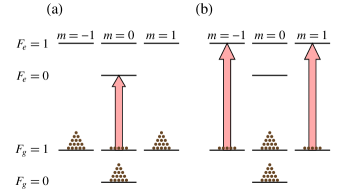
Figure 2: (Color online) Excitation with $z$-polarized light on the (a) $F_{g}=1\rightarrow F_{e}=0$ and (b) $F_{g}=1\rightarrow F_{e}=1$ transitions of a totally resolved $J_{g}=1/2\rightarrow J_{e}=1/2$ transition with $I=1/2$. Alignment is produced in the $F_{g}=1$ hyperfine level in both cases. Relative atomic populations are indicated by the number of dots displayed above each ground-state level. Relative transition strengths are indicated by the widths of the arrows—here the transition strengths are all the same.

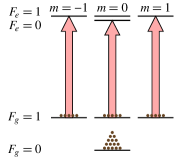
Figure 3: (Color online) As Fig. 2 but with excited-state hfs unresolved; light is resonant with the $F_{g}=1\rightarrow F_{e}$ transition group. No alignment is produced in the $F_{g}=1$ ground state.

We choose $I=1/2$ for simplicity, and the quantization axis is taken along the direction of the light polarization. In Fig. 2 the hfs is completely resolved. Part (a) of the figure shows light resonant with the $F_{g}=1\rightarrow F_{e}=0$ transition. Atoms are pumped out of the ${|F_{g}=1,m=0\rangle}$ sublevel, producing alignment in the $F_{g}=1$ state. (Linearly polarized light in the absence of other fields can only produce even-rank moments, and an $F=1$ state can only support polarization moments up to rank two; therefore, the anisotropy shown in Fig. 2 must correspond to alignment.) If light is resonant with the $F_{g}=1\rightarrow F_{e}=1$ transition, as in part (b), the ${|F_{g}=1,m=\pm 1\rangle}$ sublevels are depleted, producing alignment with sign opposite to that in Fig. 2a. This can be contrasted with the case in which the excited-state hyperfine structure is completely unresolved, shown in Fig. 3. Here, all the Zeeman sublevels of the $F_{g}=1$ state are pumped out equally—the ${|F_{g}=1,m=0\rangle}$ sublevel on the $F_{g}=1\rightarrow F_{e}=0$ transition, and the ${|F_{g}=1,m=\pm 1\rangle}$ sublevels on the $F_{g}=1\rightarrow F_{e}=1$ transition. (The relative pumping rates, which can be found from terms of the sum in Eq. (3), are all the same.) Thus no imbalance is created in the $F_{g}=1$ sublevel populations, and no polarization is created in this state.

The same principle is illustrated for nuclear spin $I=3/2$ in Fig. 4.

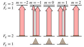
Figure 4: (Color online) Excitation with $z$-polarized light on the $F_{g}=2\rightarrow F_{e}$ transition group of a $D1$ transition with unresolved excited-state hfs. The nuclear spin is $I=3/2$. No alignment is produced in the $F_{g}=2$ hyperfine level. The width of each arrow represents the relative transition strength, which can be obtained from terms of the sum in Eq. (3).

The excited-state hfs is unresolved, and light is resonant with the $F_{g}=2\rightarrow F_{e}$ transitions. In this case, the $m=\pm 1$ ground-state sublevels are pumped on two different transitions. The total transition strength connecting each $F_{g}=2$ sublevel to the excited state is the same, and so no polarization is produced in the $F_{g}=2$ state.

The conclusions of this section must be modified when polarization produced in the ground state by spontaneous emission from the excited state is taken into account. We now consider the effect of this mechanism on the ground-state polarization (Sec. II.2).

II.2 Excited state and repopulation pumping

Through second order in the incident light field (first order in light intensity), there is one additional contribution to the ground-state polarization besides the one considered in Sec. II.1: that due to atoms being pumped to the excited state and then returning to the ground state via spontaneous emission (repopulation pumping). We first consider polarization produced in the excited state. The general form of the excited-state density matrix is Happer (1972)

$$\rho_{rs}\propto\sum_{k}{\boldsymbol{{\mathbf{\hat{e}}}}}\cdot{\boldsymbol{{\mathbf{d}}}}_{rk}{\boldsymbol{{\mathbf{\hat{e}}}}}^{\ast}\cdot{\boldsymbol{{\mathbf{d}}}}_{ks}G(\omega-\omega_{rk}),$$ (10)

where $r$ and $s$ are excited states and $k$ is a ground state. Comparing this expression to the formula for ground-state depopulation pumping [Eq. (1)], we find that, as one would expect, the roles of the ground-state and excited state have been reversed. This means that the results of Sec. II.1, with $F_{g}$ and $F_{e}$ interchanged, can be applied to the excited-state polarization. In this case, there is a limit $\kappa\leq 2J_{e}$ on the polarization moments that can be produced in the excited state, that occurs only when the ground state hfs is unresolved. The restriction does not depend on whether or not the excited-state hfs is resolved. There is the additional limit $\kappa\leq 2$ for low light power.

When the polarized atoms in the exited state decay due to spontaneous emission, the polarization can be transferred to the ground state. This contribution to the ground-state density matrix is given by Happer (1972)

$$\rho^{(repop)}_{mn}\propto\sum_{sr}{\boldsymbol{{\mathbf{d}}}}_{mr}\cdot{\boldsymbol{{\mathbf{d}}}}_{sn}\rho_{rs},$$ (11)

with $\rho_{rs}$ as given above. The fact that this formula has no reference to individual transition frequencies leads us to expect that the polarization transfer should be independent of the hyperfine splittings. Indeed, writing this expression out for the case under consideration gives

$$\begin{split}\rho^{(repop)}_{F_{g}m,F_{g}m^{\prime}}\propto&\sum(-1)^{p}{\langle F_{g}m|}d_{p}{|F_{e}m^{\prime\prime}\rangle}{\langle F_{e}m^{\prime\prime}|}\rho{|F_{e}m^{\prime\prime\prime}\rangle}\\ &\qquad\times{\langle F_{e}m^{\prime\prime\prime}|}d_{-p}{|F_{g}m^{\prime}\rangle},\end{split}$$ (12)

and the only restriction to be obtained is $m^{\prime}-m=m^{\prime\prime\prime}-m^{\prime\prime}$ (excited-state $\Delta m$ equals ground-state $\Delta m$) Cohen-Tannoudji (1962a, b). (Transforming to the uncoupled basis does not result in any additional limits.) In other words, if the polarization moment can be supported in the ground state, it can be transferred from the excited state via spontaneous emission.

Combining these results, we see that there is a similar restriction on polarization created in the ground state by repopulation pumping as the one on polarization created by depopulation pumping. However, the restriction occurs in the opposite case. When the ground state is unresolved the polarization produced by repopulation pumping must have $\kappa\leq 2J_{e}$. This limit does not depend on whether the excited-state hfs is resolved.

We now illustrate the foregoing for a system with $J_{g}=J_{e}=I=1/2$ pumped with linearly polarized light. In Fig. 5 both the ground- and excited-state hfs is resolved, and light is tuned to the $F_{g}=1\rightarrow F_{e}=1$ transition.

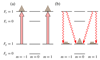
Figure 5: (Color online) Level diagram for an $D1$ transition with resolved hfs for an atom with $I=1/2$ showing (a) optical excitation and (b) spontaneous decay with linearly polarized light resonant with the $F_{g}=1\rightarrow F_{e}=1$ transition. The branching ratio for each allowed decay is the same, leading to an excess of atoms in the ${|F_{g}=1,m=0\rangle}$ sublevels over the populations of the ${|F_{g}=1,m=\pm 1\rangle}$ sublevels by a ratio of 2:1.

In part (a) of the figure, the pump light produces polarization in the $F_{e}=1$ excited state. In part (b) the excited atoms spontaneously decay. This creates polarization in the $F_{g}=1$ ground state, because more atoms are transferred to the ${|F_{g}=1,m=0\rangle}$ sublevel than to the ${|F_{g}=1,m=\pm 1\rangle}$ sublevels. (In this and the following two figures, we do not show the atoms that decay to the $F_{g}=0$ state.) Figure 6 is the same but with light tuned to the $F_{g}=0\rightarrow F_{e}=1$ transition; polarization is also created in the $F_{g}=1$ ground state in this case.

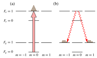
Figure 6: (Color online) As Fig. 5, but with light tuned to the $F_{g}=0\rightarrow F_{e}=1$ transition. In this case an excess of atoms results in the $m=\pm 1$ states, so that the polarization has the opposite sign as that in Fig. 5.

In Fig. 7 the ground-state hfs is now unresolved, while the excited-state hfs remains resolved.

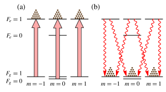
Figure 7: (Color online) As Fig. 5 but with unresolved ground-state hfs; light is tuned to the $F_{g}\rightarrow F_{e}=1$ transition group. The contributions to the ground-state polarization illustrated in Figs. 5 and 6 cancel, so that no ground-state polarization is produced.

In this case, both ground-state hyperfine levels are pumped by the light, and equal populations are produced in the sublevels of the $F_{e}=1$ state, as shown in part (a) of the figure. As seen in part (b), the excited-state atoms spontaneously decay in equal numbers to the $F_{g}=1$ sublevels, so that no polarization is produced in the $F_{g}=1$ state.

Note that in the opposite case, with unresolved excited-state hfs and resolved ground-state hfs, spontaneous decay is not prevented from producing polarization in the $F_{g}=1$ ground state.

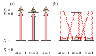
Figure 8: As Fig. 5 but with unresolved excited-state hfs; light is tuned to the $F_{g}=1\rightarrow F_{e}$ transition group. Three decay channels transfer atoms to the ${|F_{g}=1,m=0\rangle}$ sublevels, while the ${|F_{g}=1,m=\pm 1\rangle}$ sublevels are each fed by two decay channels. Since all the branching ratios are the same, the resulting population imbalance is 3:2.

In this case, atoms are pumped into the $F_{e}=0$ state, as well as the $F_{e}=1$ state, as shown in Fig. 8a. Since the ${|F_{e}=0,m=0\rangle}$ state decays isotropically, the decay from this state does not cancel out the polarization created by decay from the $F_{g}=1$ state (Fig. 8b). Thus we see that it is the ground-state hfs, and not the excited-state hfs, that needs to be resolved in order for polarization to be produced in the ground state due to spontaneous decay.

To summarize the results obtained so far, to lowest order in the excitation light, polarization can be either produced in the ground state directly through absorption, or transferred to the ground state by spontaneous emission. To this order, polarization moments due to both of these mechanisms must have rank $\kappa\leq 2$. In addition, if the excited-state hfs is unresolved, there is a limit $\kappa\leq 2J_{g}$ on the ground-state polarization due to depopulation, but no additional limit on the polarization due to repopulation. On the other hand, if the ground-state hfs is unresolved, there is a limit $\kappa\leq 2J_{e}$ on the ground-state polarization due to repopulation, but no additional limit on polarization due to depopulation. Thus, unless both the excited-state and ground-state hyperfine structure is unresolved, one or the other of the mechanisms is capable of producing polarization of all ranks $\kappa\leq 2$.

II.3 Light absorption

The absorption $\mathcal{A}$ of a weak probe light beam is given in terms of the ground-state density matrix by Happer (1972)

$$\mathcal{A}\propto\sum_{mnr}{\boldsymbol{{\mathbf{\hat{e}}}}}\cdot{\boldsymbol{{\mathbf{d}}}}_{rm}\rho_{mn}{\boldsymbol{{\mathbf{\hat{e}}}}}^{\ast}\cdot{\boldsymbol{{\mathbf{d}}}}_{nr}G(\omega-\omega_{rm}),$$ (13)

or

$$\begin{split}\mathcal{A}\propto\sum{\langle F_{e}m|}{\boldsymbol{{\mathbf{\hat{e}}}}}\cdot{\boldsymbol{{\mathbf{d}}}}{|F_{g}m^{\prime}\rangle}{\langle F_{g}m^{\prime}|}\rho{|F_{g}m^{\prime\prime}\rangle}{\langle F_{g}m^{\prime\prime}|}{\boldsymbol{{\mathbf{d}}}}\cdot{\boldsymbol{{\mathbf{\hat{e}}}}}^{\ast}{|F_{e}m\rangle}G(\omega-\omega_{F_{e}F_{g}}),\end{split}$$ (14)

where all quantities are as defined above. Using the approximation, as in Secs. II.1 and II.2, that the light is resonant with an unresolved transition group and far detuned from all other transitions, this formula reduces to

$$\begin{split}\mathcal{A}\propto\sum{\langle F_{e}m|}{\boldsymbol{{\mathbf{\hat{e}}}}}\cdot{\boldsymbol{{\mathbf{d}}}}{|F_{g}m^{\prime}\rangle}{\langle F_{g}m^{\prime}|}\rho{|F_{g}m^{\prime\prime}\rangle}{\langle F_{g}m^{\prime\prime}|}{\boldsymbol{{\mathbf{d}}}}\cdot{\boldsymbol{{\mathbf{\hat{e}}}}}^{\ast}{|F_{e}m\rangle},\end{split}$$ (15)

where the sum over $F_{g}$ and $F_{e}$ includes only those combinations that are in the unresolved resonant transition group.

We now investigate the dependence of the absorption on the ground-state polarization in various cases. Consider the case in which the ground-state hfs is completely resolved, and the excited-state structure is unresolved. The light is tuned to a unresolved transition group consisting of transitions between one ground-state hyperfine level $F_{g}$ and all of the excited-state levels. The sum in Eq. (15) over the excited states is then a closure relation, and can be replaced with a sum over any complete basis for the excited state, in particular, the uncoupled basis. We also insert closure relations to expand the ground states ${\langle F_{g}m^{\prime\prime}|}$ and ${|F_{g}m^{\prime}\rangle}$ in the uncoupled basis. We obtain

$$\begin{split}\mathcal{A}&\propto\sum(-1)^{q^{\prime}+q^{\prime\prime}}e_{q^{\prime}}(e^{\ast})_{q^{\prime\prime}}{\langle Im_{I}J_{e}m_{J}|}d_{-q^{\prime}}{|Im_{I}^{\prime}J_{g}m_{J}^{\prime}\rangle}{\langle Im_{I}^{\prime}J_{g}m_{J}^{\prime}|F_{g}m^{\prime}\rangle}{\langle F_{g}m^{\prime}|}\rho{|F_{g}m^{\prime\prime}\rangle}{\langle F_{g}m^{\prime\prime}|Im_{I}^{\prime\prime}J_{g}m_{J}^{\prime\prime}\rangle}\\ &\qquad\qquad\qquad\qquad\qquad\times{\langle Im_{I}^{\prime\prime}J_{g}m_{J}^{\prime\prime}|}d_{-q^{\prime\prime}}{|Im_{I}J_{e}m_{J}\rangle}\\ &=\sum(-1)^{q^{\prime}+q^{\prime\prime}}e_{q^{\prime}}(e^{\ast})_{q^{\prime\prime}}{\langle J_{e}m_{J}|}d_{-q^{\prime}}{|J_{g}m_{J}^{\prime}\rangle}{\langle Im_{I}J_{g}m_{J}^{\prime}|F_{g}m^{\prime}\rangle}{\langle F_{g}m^{\prime}|}\rho{|F_{g}m^{\prime\prime}\rangle}{\langle F_{g}m^{\prime\prime}|Im_{I}J_{g}m_{J}^{\prime\prime}\rangle}{\langle J_{g}m_{J}^{\prime\prime}|}d_{-q^{\prime\prime}}{|J_{e}m_{J}\rangle},\end{split}$$ (16)

where only one nuclear-spin summation variable remains in the last line. The dipole matrix element selection rules and Clebsch-Gordan conditions require that

$$\begin{gathered}m^{\prime}=m_{I}+m^{\prime}_{J},\ m^{\prime}_{J}=m_{J}+q^{\prime},\\ m^{\prime\prime}=m_{I}+m^{\prime\prime}_{J},\ m_{J}=m^{\prime\prime}_{J}+q^{\prime\prime},\end{gathered}$$ (17)

must be satisfied in order for a term in the sum to contribute to the absorption. These conditions can be combined to yield $\left|m^{\prime}-m^{\prime\prime}\right|=\left|q^{\prime}+q^{\prime\prime}\right|\leq 2$. Thus only coherences with $\left|\Delta m\right|\leq 2$ (and polarization moments with $\kappa\leq 2$) can affect the lowest-order absorption signal. The reason for this is analogous to the reason that polarization moments of maximum rank two can be created with a lowest-order interaction with the light. Absorption occurs when an atom is transferred to the excited state, i.e., when population (rank zero polarization) is created in the excited state. Thus, to be observed in the signal, a ground-state atomic PM must be coupled to a $\kappa=0$ excited-state PM by a spin-one photon, which can support polarization moments up to rank two. The triangle condition for tensor products then implies that the rank of the atomic polarization moment must be no greater than two.

Another restriction on the coherences that can affect absorption can be found from Eq. (17) by using the fact that $|m_{J}^{\prime}|\leq J_{g}$ and $|m_{J}^{\prime\prime}|\leq J_{g}$. We find

$$\left|m^{\prime}-m^{\prime\prime}\right|=\left|m^{\prime}_{J}-m^{\prime\prime}_{j}\right|\leq 2J_{g}.$$ (18)

In other words, only polarization moments with $\kappa\leq 2J_{g}$ can affect the absorption signal, regardless of the value of $F_{g}$. Evidently, it is the excited-state hfs that determines which ground-state polarization moments can be detected in absorption, whether or not the ground-state hfs is resolved.

Considering the case in which both the excited- and ground-state hfs is entirely unresolved can lend some insight into this result. In this case, every combination of $F_{g}$ and $F_{e}$ enters in the sum in Eq. (15). If the ground-state hyperfine splitting is sent to zero, the sum must be extended to include matrix elements of $\rho$ between different hyperfine levels. This means that all of the sums in Eq. (15) can be replaced with sums over uncoupled basis states, giving

$$\begin{split}\mathcal{A}&\propto\sum(-1)^{q^{\prime}+q^{\prime\prime}}e_{q^{\prime}}(e^{\ast})_{q^{\prime\prime}}{\langle Im_{I}J_{e}m_{J}|}d_{-q^{\prime}}{|Im_{I}^{\prime}J_{g}m_{J}^{\prime}\rangle}{\langle Im_{I}^{\prime}J_{g}m_{J}^{\prime}|}\rho{|Im_{I}^{\prime\prime}J_{g}m_{J}^{\prime\prime}\rangle}{\langle Im_{I}^{\prime\prime}J_{g}m_{J}^{\prime\prime}|}d_{-q^{\prime\prime}}{|Im_{I}J_{e}m_{J}\rangle}\\ &=\sum(-1)^{q^{\prime}+q^{\prime\prime}}e_{q^{\prime}}(e^{\ast})_{q^{\prime\prime}}{\langle J_{e}m_{J}|}d_{-q^{\prime}}{|J_{g}m_{J}^{\prime}\rangle}{\langle Im_{I}J_{g}m_{J}^{\prime}|}\rho{|Im_{I}J_{g}m_{J}^{\prime\prime}\rangle}{\langle J_{g}m_{J}^{\prime\prime}|}d_{-q^{\prime\prime}}{|J_{e}m_{J}\rangle}.\end{split}$$ (19)

Since the hyperfine interaction has been effectively eliminated, the absorption no longer depends on the nuclear spin: the complete density matrix does not enter, but rather the reduced density matrix

$$\rho^{(J)}_{m_{J}^{\prime}m_{J}^{\prime\prime}}=\sum_{m_{I}}\rho_{m_{I}m_{J}^{\prime},m_{I}m_{J}^{\prime\prime}}$$ (20)

that is averaged over the nuclear spin $m_{I}$. The reduced density matrix can only support polarization moments up to rank $\kappa=2J_{g}$, so any PM in $\rho$ with higher rank cannot affect the absorption. Considering a density matrix that is nonzero only within one ground-state hyperfine level $F_{g}$, we see that polarization moments with rank greater than two will not contribute to the signal. Since the other ground-state hyperfine levels are unoccupied, it makes no difference what the ground-state hyperfine splitting is, so we regain the result that, even if the ground-state hfs is resolved, only polarization moments with $\kappa\leq 2J_{g}$ can affect the absorption of light if the excited-state hfs is unresolved.

There is no corresponding restriction on the polarization moments that can affect absorption when the ground-state hfs is unresolved and the excited-state hfs is resolved. Indeed, we can consider the case in which only one ground-state hyperfine level $F_{g}$ is populated: the absorption is then exactly as if the transition $F_{g}\rightarrow F_{e}$ were completely isolated. For such an isolated transition, the only limit on detectable polarization moments is $\kappa\leq 2$ for the low-power case.

As in the previous subsections, we illustrate this result for a $D1$ transition for an atom with $I=1/2$ subject to linearly polarized light. In Fig. 9 both the ground- and excited-state hfs is resolved, and the light is resonant with the $F_{g}=1\rightarrow F_{e}=1$ transition.

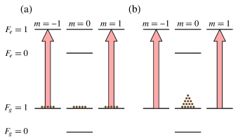
Figure 9: (Color online) $D1$ transition for an atom with $I=1/2$ subject to linearly polarized light resonant with the $F_{g}=1\rightarrow F_{e}=1$ transition. In part (a) the $F_{g}=1$ ground state is unpolarized and there is light absorption. In part (b) the $F_{g}=1$ state has the same total population, but is aligned, and there is no absorption.

In part (a) there is no polarization in the $F_{g}=1$ ground state: atoms are equally distributed among the Zeeman sublevels. Light is absorbed by atoms in the ${|F_{g}=1,m=\pm 1\rangle}$ sublevels. In part (b) there are the same total number of atoms in the $F_{g}=1$ state, but they are collected in the $m=0$ sublevel. The population is the same, but the $F_{g}=1$ state now also has alignment. In this particular case there is no absorption, because the atoms are all in the $m=0$ dark state. Thus, in this situation, the rank-two polarization moment has a strong effect on the absorption signal.

Figure 10 shows the same system, but with unresolved excited-state hfs.

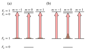
Figure 10: (Color online) As Fig. 9, but with unresolved excited-state hfs. In this case there is no difference in the absorption seen for an (a) unpolarized and (b) aligned $F_{g}=1$ ground state.

In this case there is no dark state; all of the atoms interact with the light. The distribution of the atoms among the Zeeman sublevels does not affect the light absorption, and so the rank two polarization moment is not detectable in the absorption signal.

II.4 Fluorescence

Finally, we consider which excited-state polarization moments can be observed in fluorescence. Assuming broadband detection, the intensity of fluorescence into a particular polarization ${\boldsymbol{{\mathbf{\hat{e}}}}}$ is given in terms of the excited-state density matrix by

$$\mathcal{I}\propto\sum_{rsm}{\boldsymbol{{\mathbf{\hat{e}}}}}^{\ast}\cdot{\boldsymbol{{\mathbf{d}}}}_{mr}\rho_{rs}{\boldsymbol{{\mathbf{\hat{e}}}}}\cdot{\boldsymbol{{\mathbf{d}}}}_{sm}.$$ (21)

Because the sums in $r$ and $s$ go over all excited states, and $m$ runs over all ground states, we can write Eq. (21) for our case in terms of the uncoupled-basis states. This gives

$$\mathcal{I}\propto\sum(-1)^{q^{\prime}+q^{\prime\prime}}\left(e^{\ast}\right)_{q^{\prime}}e_{q^{\prime\prime}}{\langle Im_{I}J_{g}m_{J}|}d_{-q^{\prime}}{|Im^{\prime}_{I}J_{e}m^{\prime}_{J}\rangle}{\langle Im^{\prime}_{I}J_{e}m^{\prime}_{J}|}\rho{|Im^{\prime\prime}_{I}J_{e}m^{\prime\prime}_{J}\rangle}{\langle Im^{\prime\prime}_{I}J_{e}m^{\prime\prime}_{J}|}d_{-q^{\prime\prime}}{|Im_{I}J_{g}m_{J}\rangle},$$ (22)

resulting in the restrictions

$$\begin{gathered}m^{\prime\prime}_{J}=-q^{\prime\prime}+m_{J},\ m_{J}=-q^{\prime}+m^{\prime}_{J},\\ m_{I}=m^{\prime}_{I}=m^{\prime\prime}_{I},\end{gathered}$$ (23)

on the terms that can contribute to the fluorescence. This indicates that the nuclear polarization cannot affect the fluorescence signal, and so only the electronic excited-state polarization of rank $\kappa\leq 2J_{e}$ can be observed. In addition, only coherences with $\left|m^{\prime\prime}_{J}-m^{\prime}_{J}\right|=\left|q^{\prime}+q^{\prime\prime}\right|\leq 2$ can be observed. This rule has appeared earlier as a consequence of the low-light-power assumption; because spontaneous decay is not induced by an incident light field, in this case the rule is exact. This means that no matter the value of $J_{e}$, and what polarization moments exist in the excited state, only polarization of rank $\kappa\leq 2$ can be observed in fluorescence.

II.5 Summary

In this section, we have shown that, when the ground- or excited-state hfs is unresolved, there are restrictions on the rank of the polarization moments that can be created or detected by light. Some of these restrictions may at first seem counter-intuitive, but they can be obtained from very basic considerations. For example, the two facts that nuclear spin can be ignored if the hfs is completely unresolved and that lowest-order depopulation pumping of a given hyperfine level does not depend on ground-state hyperfine splitting lead directly to the result that polarization moments produced by depopulation pumping are subject to a limit of $\kappa\leq 2J_{g}$ when the excited-state hfs is unresolved. Various processes of creation and detection of polarization are subject to different restrictions (Table 1).

	unresolved	limit on $\kappa$
Ground-state pol. (depop.)	excited hfs	$\leq 2J_{g}$
Ground-state pol. (repop.)	ground hfs	$\leq 2J_{e}$
Excited-state pol.	ground hfs	$\leq 2J_{e}$
Absorption	excited hfs	$\leq 2J_{g}$
Fluorescence	—	$\leq 2J_{e}$

Table 1: Summary of the results of this section. For each quantity, the restriction on the rank $\kappa$ of the polarization that can be created or detected is given in the third column. The restriction holds under conditions (ground- or excited-state hfs unresolved) described in the second column. For fluorescence with broad-band detection the restriction holds regardless of whether the hfs is resolved.

In particular, the two processes that can create ground-state polarization—depopulation and repopulation pumping—are subject to restrictions under different conditions. Consequently, unless the hfs is entirely unresolved, there is always a mechanism for producing polarization limited in rank only by the total angular momentum, rather than the electronic angular momentum.

III Partially resolved hyperfine structure: nonlinear magneto-optical effects

Now let us examine the more general case of partially resolved hyperfine transitions. For this study, we will look at the quantitative dependence on hyperfine splitting of nonlinear optical rotation—rotation of light polarization due to interaction with a $J_{g}\rightarrow J_{e}$ transition group in the presence of a magnetic field. In this case, the effect of ground-state atomic polarization is brought into starker relief: in the experimental situation that we consider, both the creation and detection of ground-state polarization is required in order to see any signal whatsoever. When linearly polarized light is used, as is supposed here, the lowest-order effect depends on rank-two atomic alignment. Thus, for the alkali atoms, the question of the dependence of the effect on hyperfine structure arises, because, as discussed in the previous section, both the creation and the detection of alignment in the $J_{g}=1/2$ ground state can be suppressed due to unresolved hfs. (In fact, a higher-order effect can occur wherein alignment is created, the alignment is converted to orientation, and the orientation is detected Auzinsh and Ferber (1992); Budker et al. (2000a); Auzinsh et al. (2006). However, the conversion of alignment to orientation is an effect of tensor ac Stark shifts, which can be shown by arguments similar to those in Sec. II to suffer suppression due to unresolved hfs in the same way as does the direct detection of alignment.)

In the Faraday geometry, linearly polarized light propagates in the direction of an applied magnetic field, and the rotation of the light polarization direction is measured. A number of magneto-optical effects can contribute to the optical rotation, including the linear Faraday effect, the Bennett-structure effect, and various effects depending on atomic polarization (“coherence effects”) Budker et al. (2002). Here we are concerned with optical rotation due to several different forms of the ground-state coherence effect, in which the atomic velocities are treated in three different ways. First we consider the atoms to have no velocity spread, and analyze the Doppler-free “transit effect”, as for an atomic beam with negligible transverse velocity distribution Schuh et al. (1993). We then consider the case in which atoms have a Maxwellian distribution, but do not change their velocities in between pumping and probing—this corresponds to the transit effect for buffer-gas-free, dilute atomic vapors Kanorsky et al. (1993). Finally, we treat the case in which atoms undergo velocity-changing collisions between pumping and probing, as for buffer-gas cells Novikova et al. (2001) or the wall-induced Ramsey effect (“wall effect”) in antirelaxation-coated vapor cells Kanorskii et al. (1995). Figure 11 illustrates the transit and wall effects in a vapor cell.

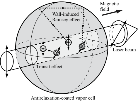
Figure 11: The transit and wall optical-rotation effects. Both effects occur in an anti-relaxation-coated vapor cell, and can be distinguished by their greatly different magnetic resonance widths.

We examine the dependence of these effects on the size of the hyperfine splittings as they vary from much smaller than the natural width to much greater than the Doppler width.

Throughout this section we consider formulas for the optical rotation signal valid to lowest order in light power, under the assumption that the ground-state relaxation rate $\gamma$ is much smaller than both the excited-state natural width $\Gamma$ and the hyperfine splittings. For the Doppler-free case a single analytic formula can be applied to both resolved and unresolved hfs (i.e., no assumption need be made about the relative size of the hyperfine splittings and the natural width). For the Doppler-broadened cases, analytic results can be obtained in various limits, which together describe the signal over the entire range of hyperfine splittings.

We first focus on the simplest case: the $D1$ line ($J_{g}=J_{e}=1/2$) for an atom with $I=1/2$. This is a somewhat special case, because one of the two ground-state hyperfine levels has $F_{g}=0$, and consequently can neither support atomic alignment nor produce optical rotation. We then consider the differences that arise when considering higher nuclear spin and also the $D2$ line ($J_{g}=1/2$ and $J_{e}=3/2$). Finally, results for the “real-world” alkali atoms commonly used in experiments are presented. Some details of the calculation and general formulas for arbitrary $J_{g}$, $J_{e}$, and $I$ are presented in Appendix A. These formulas are generalizations of those given in Ref. Kanorsky et al. (1993); related earlier work includes that of Refs. Happer and Mathur (1967); Mathur et al. (1970).

III.1 Doppler-free transit effect

We consider nonlinear Faraday rotation on a $J_{g}\rightarrow J_{e}$ atomic transition for an atom with nuclear spin $I$. We can limit our attention to the ground-state coherence effects by using a “three-stage” model for Faraday rotation Kanorsky et al. (1993), in which optical pumping, atomic precession, and optical probing take place sequentially, and the light and magnetic fields are never present at the same time. In this case, the linear and Bennett-structure effects, which require the simultaneous application of light and magnetic fields, do not occur. Such a model can be realized in an atomic beam experiment, but it is also a good approximation to a vapor cell experiment that uses low light power and small enough magnetic fields so that the coherence effects are dominant.

The calculation is performed using second order perturbation theory in the basis of the polarization moments $\rho^{(\kappa q)}(F_{1}F_{2})$ of the density matrix (Appendix A.1). The three stages of the calculation are as follows. In stage (a), a $x$-directed light beam linearly polarized along $z$ is applied, and we calculate optical pumping through second order in the optical Rabi frequency. In stage (b), the light field is removed, and a $x$-directed magnetic field is applied. We calculate the effect of this field on the atomic polarization. Finally, in stage (c), the magnetic field is turned off, and the light field is applied once more to probe the atomic polarization. The nonlinear optical rotation is found to lowest order in the probe-light Rabi frequency (Appendix A.2).

Because the magnetic field is neglected during the optical pumping stage, the atomic ground-state polarization that is produced in this stage is entirely along the light polarization direction, i.e., it has polarization component $q=0$. Since linearly polarized light has a preferred axis, but no preferred direction, it can not, in the absence of other fields, produce atomic polarization with a preferred direction, i.e., polarization with odd rank $\kappa$. Also, we have seen in Sec. II that, to lowest order in the light power, optical pumping cannot produce polarization moments with $\kappa>2$. Thus the only ground-state polarization moment with rank greater than zero that is produced at lowest order has $\kappa=2$ and $q=0$. We first consider the $D1$ line ($J_{g}=J_{e}=1/2$) for an atom with $I=1/2$. In this case, the only ground-state hyperfine level that can support the $\rho^{(20)}(F_{g}F_{g})$ moment has $F_{g}=1$. (Due to the assumption that the hyperfine splittings are much greater than the ground-state relaxation rate, we can ignore ground-state hyperfine coherences throughout the discussion.) From Eq. (60), the value of this moment is found to be

$$\begin{split}\rho^{(20)}(11)&=\frac{\kappa_{s}}{12\sqrt{6}}\Big{(}\left[L(\omega^{\prime}_{0,1})-L(\omega^{\prime}_{1,1})\right]\\ &\qquad\qquad\qquad+\frac{R}{3}\left[L(\omega^{\prime}_{1,0})-L(\omega^{\prime}_{1,1})\right]\Big{)},\end{split}$$ (24)

where $\kappa_{s}=(J_{g}\|d\|J_{e})^{2}\mathcal{E}_{0}^{2}/(\Gamma\gamma)$ is the reduced optical-pumping saturation parameter ($\mathcal{E}_{0}$ is the optical electric field amplitude), $R$ is the branching ratio for the transition $J_{e}\rightarrow J_{g}$, and $\omega^{\prime}_{F_{e}F_{g}}$ is the transition frequency between excited-state and ground-state hyperfine levels in the frame “rotating” at the Doppler-shifted light frequency $\omega$: $\omega^{\prime}_{F_{e}F_{g}}=\omega_{F_{e}F_{g}}-\omega+{\boldsymbol{{\mathbf{k}}}}\cdot{\boldsymbol{{\mathbf{v}}}}$, where $\omega_{F_{e}F_{g}}$ is the transition frequency in the lab frame, $\omega$ is the light frequency, ${\boldsymbol{{\mathbf{k}}}}$ is the wave vector, and ${\boldsymbol{{\mathbf{v}}}}$ is the atomic velocity. We also write $\omega^{\prime}_{F_{e}F_{g}}=-\Delta_{F_{e}F_{g}}+{\boldsymbol{{\mathbf{k}}}}\cdot{\boldsymbol{{\mathbf{v}}}}$, where $\Delta_{F_{e}F_{g}}$ is the light detuning from resonance. We have defined the Lorentzian line profile

$$L(\omega^{\prime})=\frac{(\Gamma/2)^{2}}{(\Gamma/2)^{2}+\omega^{\prime 2}}.$$ (25)

Equation (24) is written as the sum of two terms, each surrounded by square brackets. The first term is the contribution to the polarization due to depopulation pumping discussed in Sec. II.1. This term is itself a sum of contributions due to pumping on the $F_{g}=1\rightarrow F_{e}=0$ transition and the $F_{g}=1\rightarrow F_{e}=1$ transition. These two contributions are of opposite sign, as illustrated in Fig. 2. Pumping on either transition produces alignment in the $F_{g}=1$ ground state; the sign of the corresponding polarization moment depends on whether there is more population in the $m=0$ sublevel or the $m=\pm 1$ sublevels. We saw in the discussion of Sec. II.1 that when the excited state hfs is unresolved, polarization with rank $\kappa>2J_{g}$ cannot be created by depopulation pumping (Fig. 3). We see here that as $\omega_{0,1}$ approaches $\omega_{1,1}$, i.e., as the excited-state hyperfine splitting goes to zero, the contributions from the two transitions cancel and this term goes to zero. For the Doppler-broadened atomic ensemble discussed in Sec. II, the hfs was considered unresolved when the hyperfine splittings were smaller than the Doppler width. Since Eq. (24) describes a single velocity group, the relevant width here is the natural width $\Gamma$.

The second term of Eq. (24) is the contribution to the ground-state polarization due to repopulation pumping discussed in Sec. II.2. This term is also composed of two contributions of opposite sign: one due to pumping on the $F_{g}=1\rightarrow F_{e}=1$ transition and one due to pumping on the $F_{g}=0\rightarrow F_{e}=1$ transition. The two contributions are illustrated in Figs. 5 and 6, which show the origin of the opposite signs. In Sec. II.2 we found that depopulation pumping cannot create polarization moments with rank $\kappa>2J_{e}$ when the ground-state hfs is unresolved (Fig. 7). We see here that this term of Eq. (24) goes to zero when $\omega_{1,0}$ approaches $\omega_{1,1}$, i.e., as the ground-state hyperfine splitting goes to zero.

In the second and third stages of the model of the coherence effect, the ground-state polarization precesses in a magnetic field and is probed by light with the same polarization as the pump light considered in the first stage. From Eq. (72) we find that the normalized optical rotation $d\varphi$ per path length $d\ell$ is proportional to the polarization produced in the first stage and is given by

$$\ell_{0}\frac{d\varphi}{d\ell}=\frac{1}{4}\sqrt{\frac{3}{2}}\left[L(\omega^{\prime}_{0,1})-L(\omega^{\prime}_{1,1})\right]x_{1}\rho^{(20)}(11),$$ (26)

where

$$x_{F_{g}}=\frac{(\gamma/2)\Omega_{F_{g}}}{(\gamma/2)^{2}+\Omega_{F_{g}}^{2}}$$ (27)

is the magnetic-resonance line-shape parameter, with $\Omega_{F_{g}}=g_{F_{g}}\mu_{B}B$ the Larmor frequency for the ground-state hyperfine level $F_{g}$ ($g_{F_{g}}$ is the Landé factor for the ground state $F_{g}$, and $\mu_{B}$ is the Bohr magneton), and

$$\ell_{0}=-\left(\frac{1}{\mathcal{I}}\frac{d\mathcal{I}}{d\ell}\right)^{-1}=\frac{2\pi}{Rn\lambda^{2}}\frac{(2J_{g}+1)}{(2J_{e}+1)}$$ (28)

is the unsaturated resonant absorption length assuming totally unresolved hyperfine structure, where $\mathcal{I}$ is the light intensity, $n$ is the atomic density, and $\lambda$ is the light wavelength. The branching ratio $R$ enters here because it factors into the transition strength.

The contributions to the optical rotation signal from the $F_{g}=1\rightarrow F_{e}=0$ transition and the $F_{g}=1\rightarrow F_{e}=1$ transition have opposite signs. To understand this, it is helpful to think of the optically polarized medium as a polarizing filter Kanorsky et al. (1993). When pumping on a $1\rightarrow 0$ or $1\rightarrow 1$ transition, the medium is pumped into a dark (non-absorbing) state for that transition (Fig. 2), corresponding to a polarizing filter with its transmission axis along the input light polarization axis ${\boldsymbol{{\mathbf{\hat{e}}}}}$ [Fig. 12(a)].

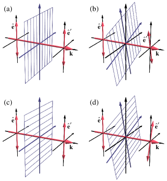
Figure 12: Illustration of the rotating polarizer model for optical rotation. (a) Optical pumping on a $F_{g}=1\rightarrow F_{e}=0$ or $F_{g}=1\rightarrow F_{e}=1$ transition causes the medium to act as a polarizing filter with transmission axis along the input light polarization ${\boldsymbol{{\mathbf{\hat{e}}}}}$. (b) When the transmission axis rotates due to Larmor precession, the output light polarization ${\boldsymbol{{\mathbf{\hat{e}}}}}^{\prime}$ follows the transmission axis and so rotates in the same sense as the Larmor precession. (c) If polarization produced by pumping on one transition is probed on the other, the polarization functions as a polarizing filter with transmission axis perpendicular to the input light polarization. (Attenuation of the light beam is not indicated.) (d) When the medium polarization rotates, the output light polarization tends to rotate towards the transmission axis, in the opposite sense to the Larmor precession in this case.

The Larmor precession induced by the magnetic field causes the transmission axis of the filter to rotate, so that it is no longer along ${\boldsymbol{{\mathbf{\hat{e}}}}}$. This in turn causes the output light polarization axis ${\boldsymbol{{\mathbf{\hat{e}}}}}^{\prime}$ to rotate. The polarization of light passing through a polarizing filter tends to rotate towards the transmission axis, so that in this case the optical rotation is in the same sense as the Larmor precession [Fig. 12(b)]. Now, compare the polarization produced when pumping on a $1\rightarrow 0$ or $1\rightarrow 1$ transition, as shown in Fig. 2. We see that the dark state for each transition is a bright (absorbing) state for the other. This means that if we choose one or the other of these states, it will function as just described for one of the transitions, but will function as a polarizing filter with its transmission axis perpendicular to ${\boldsymbol{{\mathbf{\hat{e}}}}}$ for the other transition [Fig. 12(c)]. When the axis of the filter rotates in this case, the fact that the output light polarization tends to rotate towards the transmission axis, means that here the optical rotation is in the other direction, in the opposite sense to the Larmor precession [Fig. 12(d)]. In other words, for a particular sign of the rank-two polarization moment, the optical rotation will have one sign when probed on one transition, and the opposite sign when probed on the other, as indicated by Eq. (26). Because the observation of optical rotation requires the detection of rank-two polarization moments, we might expect, analogously to the discussion in Sec. II.3, that it is suppressed when the excited-state hyperfine splitting goes to zero. Equation (26) shows that the two contributions indeed cancel when $\omega_{0,1}$ approaches $\omega_{1,1}$.

Equation (26) and the two components of Eq. (24) are plotted as a function of light detuning from the $F_{g}=1\rightarrow F_{e}=1$ transition in Fig. 13, for particular values of the ground- and excited-state hyperfine coefficients $A_{g}$ and $A_{e}$.

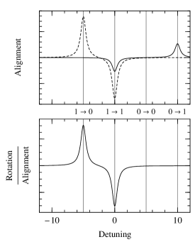
Figure 13: Dependence on light detuning from the $F_{g}=1\rightarrow F_{e}=1$ transition of (top) the components of ground-state alignment due to depopulation (dashed) and repopulation (solid) [Eq. (24)] and (bottom) optical rotation for a given amount of alignment [Eq. (26)]. Gray vertical lines show $F_{g}\rightarrow F_{e}$ transition resonance frequencies. Parameter values in units of $\Gamma$ are $\gamma\ll 1$, $A_{g}=10$, $A_{e}=5$.

(For $J=I=1/2$, the hyperfine coefficient $A$ is equal to the splitting between the two hyperfine levels.) Here and below numerical values of frequencies are given in units of $\Gamma$. As discussed above, each spectrum consists of two peaks of equal magnitude and opposite sign. For the spectrum of alignment due to depopulation and the spectrum of rotation for a given amount of alignment, the peaks are separated by the excited-state hyperfine splitting, so that they cancel as this splitting goes to zero. For the spectrum of alignment due to repopulation, the peaks are separated by the ground-state hyperfine splitting; they cancel as the ground-state splitting goes to zero.

In this subsection we are analyzing a Doppler-free system, i.e., we assume that the atoms all have the same velocity, which we take to be zero for simplicity. Then the observed optical rotation signal is found by simply substituting Eq. (24) into Eq. (26). We first consider the case in which the ground-state hfs is well resolved. The rotation signal is plotted in Fig. 14 for large ground-state hyperfine splitting and various excited-state splittings $A_{e}$.

Figure 14: Spectra of normalized optical rotation $\ell_{0}/(\kappa_{s}x_{1})(d\varphi/d\ell)$ for the Doppler-free transit effect. Left column: components due to polarization produced by depopulation (dashed) and repopulation (solid); right column: total signal. Parameter values in units of $\Gamma$ are $\gamma\ll 1$, $A_{g}\gg 1,A_{e}$.

The components of the rotation signal due to depopulation (dashed) and repopulation (solid) are plotted in the left-hand column, and the total signal is plotted on the right. As the previous discussion indicates, the rotation signal decreases as the excited-state hyperfine splitting $A_{e}$ becomes smaller, with the component due to depopulation decreasing faster than the component due to repopulation. This is also seen in Fig. 15, which shows the maximum magnitude of the rotation spectrum as a function of $A_{e}$ (for each value of $A_{e}$, the signal is optimized with respect to detuning).

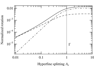
Figure 15: Maximum of the spectrum of the Doppler-free nonlinear magneto-optical rotation transit effect as a function of excited-state hyperfine splitting. Plotted are the component due to polarization produced by depopulation (dash-dotted) due to polarization produced by repopulation (dashed) and the total signal (solid). Parameters as in Fig. 14.

Thus, for small splittings, the component due to repopulation dominates. To lowest order in $A_{e}$, the signal is given by

$$\ell_{0}\frac{d\varphi}{d\ell}=\frac{A_{e}\kappa_{s}x_{1}R(\Gamma/2)^{4}\Delta_{1}}{144\left[(\Gamma/2)^{2}+\Delta_{1}^{2}\right]^{3}},$$ (29)

i.e., linear in $A_{e}$, with a modified dispersive shape that falls off far from resonance as $1/\Delta_{1}^{5}$, where $\Delta_{1}$ is the detuning from the center of the $F_{g}=1\rightarrow F_{e}$ transition group.

The previous discussion also explains why the two peaks in the component due to depopulation seem to cancel as they overlap, even though they have the same sign: the factors in the signal due to the creation and detection of alignment cancel individually (Fig. 13); it is only in their product that the two peaks have the same sign.

We now consider the case in which both the ground- and excited-state hyperfine splittings are small, so that all of the hfs is unresolved. To lowest order in $A_{g}$ and $A_{e}$ we have

$$\ell_{0}\frac{d\varphi}{d\ell}=A_{e}\left(A_{e}-\frac{R}{3}A_{g}\right)\frac{\kappa_{s}x_{1}(\Gamma/2)^{4}\Delta^{2}}{24\left[(\Gamma/2)^{2}+\Delta^{2}\right]^{4}},$$ (30)

where $\Delta$ is the light detuning from the line center of the $D1$ transition. As we expect, the component of the signal due to polarization produced by repopulation is proportional to $A_{g}$ for small hyperfine splitting. The component of the signal resulting from depopulation-induced polarization also enters at this order. The optical rotation spectrum in this case is double-peaked, and falls off as $1/\Delta^{6}$ (Fig. 16).

Figure 16: As Fig. 14, with $A_{g}$ and $A_{e}$ varied simultaneously ($A_{g}=20A_{e}$).

III.2 Doppler-broadened transit effect

We now consider an atomic ensemble with a Maxwellian velocity distribution, but a low rate of velocity-changing collisions, so that the atomic velocities do not change between optical pumping and probing. This is the case for an atomic beam experiment, or for the “transit effect” in a dilute-vapor cell. Because the atoms have a fixed velocity, the signal from each velocity group can be found individually and then summed to find the total signal. Thus the signal from the Doppler-broadened transit effect is found by multiplying the Doppler-free signal found in the previous subsection by a Gaussian weighting function representing the Doppler distribution along the light propagation direction and then integrating over atomic velocity. We can perform this integral analytically in different limiting cases.

We first consider the commonly encountered experimental case in which the hyperfine splitting is much greater then the natural line width of the excited state, i.e., the Doppler-free spectrum is well resolved. In this case, for a given light frequency and atomic velocity, the light acts on at most one transition between hyperfine levels. Thus the excited-state hyperfine coherences can be neglected, and the cancelation effects due to the overlap of resonance lines do not appear. As found in Eq. (74), the Doppler-free rotation spectrum then appears as a collection of peaks, one centered at each optical resonance frequency, each with line-shape function $f(\omega_{F_{e}F_{g}}^{\prime})=L(\omega_{F_{e}F_{g}}^{\prime})^{2}$, i.e., the square of a Lorentzian line shape. (One Lorentzian factor is due to optical pumping, the other to probing.)

In this case, the Doppler-broadened signal is found by making the replacement $f\rightarrow f_{DB}$, where the velocity integral for $f_{DB}$ takes the form

$$f_{DB}(\Delta_{F_{e}F_{g}})=\int dv_{k}f(-\Delta_{F_{e}F_{g}}+k_{B}v_{k})G(v_{k}),$$ (31)

where

$$G(v_{k})=\frac{k_{B}}{\Gamma_{D}\sqrt{\pi}}e^{-(k_{B}v_{k}/\Gamma_{D})^{2}}$$ (32)

is the normalized distribution of atomic velocities along the light propagation direction ${\boldsymbol{{\mathbf{\hat{k}}}}}$, $k_{B}$ is the Boltzmann constant, and $\Gamma_{D}$ is the Doppler width. This integral can be evaluated in terms of the error function. Under the assumption $\Gamma\ll\Gamma_{D}$ that we will employ here, the integral can be approximated by replacing $f$ with a properly normalized delta function, resulting in

$$f_{DB}(\Delta_{F_{e}F_{g}})\approx\frac{\sqrt{\pi}}{4}\frac{\Gamma}{\Gamma_{D}}e^{-(\Delta_{F_{e}F_{g}}/\Gamma_{D})^{2}}.$$ (33)

The Doppler-broadened spectrum, given explicitly by Eq. (75), thus consists of a collection of resonances, each with Gaussian line shape. For the $D1$ line with $I=1/2$, we have

$$\ell_{0}\frac{d\varphi}{d\ell}=\frac{\kappa_{s}x_{1}}{576}\left((3+R)e^{-(\Delta_{1,1}/\Gamma_{D})^{2}}+3e^{-(\Delta_{0,1}/\Gamma_{D})^{2}}\right).$$ (34)

Here $\ell_{0}$ is the absorption length for the Doppler-broadened case, given by

$$\ell_{0}=\frac{4\sqrt{\pi}}{Rn\lambda^{2}}\frac{\Gamma_{D}}{\Gamma}\frac{(2J_{g}+1)}{(2J_{e}+1)}.$$ (35)

Equation (34) is valid for $A_{e},A_{g},\Gamma_{D}\gg\Gamma$. Note that all the terms in this expression have the same sign; thus no cancelation occurs when the resonances overlap. This is because the Doppler-free resonances all have the same sign when the Doppler-free spectrum is well resolved (Fig. 14), so when the Doppler-broadened spectrum samples more than one resonance, the contributions from each resonance add.

The same approach can be generalized to describe the case in which some or all of the hyperfine splittings are on the order of or smaller than $\Gamma$. In this case, the Doppler-free spectrum is not composed entirely of peaks with a shape given by $f(\omega_{F_{e}F_{g}}^{\prime})$. Nevertheless, as long as each resonance or group of resonances has frequency extent much less than the Doppler width, we can approximate it as a delta function times a coefficient given by the integral of the Doppler-free spectrum over the resonance. For the $D1$ line with $I=1/2$ and $A_{e},\Gamma\ll\Gamma_{D}\ll A_{g}$, this procedure yields [Eq. (76)]

$$\ell_{0}\frac{d\varphi}{d\ell}=\frac{A_{e}^{2}\kappa_{s}x_{1}(6+R)e^{-\Delta_{1,1}^{2}/\Gamma_{D}^{2}}}{576\left(\Gamma^{2}+A_{e}^{2}\right)}.$$ (36)

The rotation in this case goes as $A_{e}^{2}$ for small $A_{e}$; the term linear in $A_{e}$ [Eq. (29)] is odd in detuning and consequently cancels in the velocity integral.

Since Eq. (34) applies when $A_{e}\gg\Gamma$ and Eq. (36) applies when $A_{e}\ll\Gamma_{D}$, we have that—if $\Gamma_{D}$ is sufficiently larger than $\Gamma$—the two formulas together describe the signal over the entire range of $A_{e}$ to excellent approximation, as verified by a numerical calculation. Figure 17 shows the maximum of the rotation spectrum as a function of the excited-state hyperfine splitting.

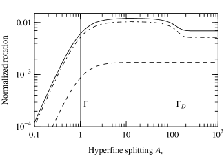
Figure 17: Maximum of the spectrum of the Doppler-broadened effect as a function of excited-state hyperfine splitting. Plotted are the component due to polarization produced by depopulation (dash-dotted), due to polarization produced by repopulation (dashed), and the total signal (solid). Equation (36) is used for $A_{e}<10$, and Eq. (34) is used for $A_{e}>10$. Parameter values in units of $\Gamma$ are $\Gamma_{D}=100$, $\gamma\ll 1$, $A_{g}\gg\Gamma_{D}$.

As discussed above, as $A_{e}$ is reduced, there is no suppression of the optical rotation signal when the Doppler-broadened hfs becomes unresolved. Only when the Doppler-free spectrum for a particular velocity group becomes unresolved is there suppression, as described in the previous subsection.

Spectra for the Doppler-broadened transit effect are shown in Fig. 18 for large $A_{g}$ and various values of $A_{e}$, and for $A_{g}$ and $A_{e}$ varied together in Fig. 19.

Figure 18: Spectra, as Fig. 14, but for the Doppler-broadened transit effect. Parameter values in units of $\Gamma$ are $\Gamma_{D}=100$, $\gamma\ll 1$, $A_{g}\gg\Gamma_{D}$.

Figure 19: As Fig. 18, with $A_{g}$ and $A_{e}$ varied simultaneously ($A_{g}=20A_{e}$).

In the case in which both $A_{e}$ and $A_{g}$ are small, the Doppler-free rotation spectrum is entirely of the same sign [see Eq. (30) and the bottom plot of Fig. 16]. The Doppler-broadened signal thus behaves similarly to the Doppler-free signal, because no additional cancelation takes place upon integrating over the velocity distribution. The signal for the $D1$ line with $I=1/2$ and $A_{g},A_{e},\Gamma\ll\Gamma_{D}$ is given by

$$\ell_{0}\frac{d\varphi}{d\ell}=A_{e}\left(A_{e}-\frac{R}{3}A_{g}\right)\frac{\kappa_{s}x_{1}}{96\,\Gamma^{2}}e^{-\Delta^{2}/\Gamma_{D}^{2}}.$$ (37)

III.3 Wall effect

We now consider systems in which the atomic velocities change in between optical pumping and probing. This is the case for the “wall effect” in antirelaxation-coated vapor cells: atoms are optically pumped as they pass through the light beam, and then retain their polarization through many collisions with the cell walls before returning to the beam and being probed (Fig. 11). A similar situation occurs in vapor cells with buffer gas.

We assume that the atomic velocities are completely randomized after optical pumping. Then the density matrix for each velocity group is the same; to lowest order in light power, we can find the velocity-averaged polarization by integrating the perturbative expression (60) over velocity with the Gaussian weighting factor (32). Since we are now describing the average over all of the atoms in the cell, and not just the illuminated region of the cell, we take $\gamma$ to be the average ground-state relaxation rate for an atom in the cell, rather than the transit rate through the light beam. We also multiply the polarization by the illuminated fraction of the cell volume, $V_{\text{illum.}}/V_{\text{cell}}$ (assuming this fraction is small), to account for the fact that the light pumps only some of the atoms at a time.

For the specific case of the $D1$ line for an atom with $I=1/2$, Eq. (60) takes the form, given in Eq. (24), of a linear combination of Lorentzian functions $L(\omega_{F_{e}F_{g}}^{\prime})$. This simple form arises because, due to the selection rules for this transition, no coherences are formed between excited-state hyperfine levels. For a general system this is not the case; however, if the excited-state hyperfine splitting is greater than $\Gamma$, the excited-state hyperfine coherences are suppressed, and all resonances once again have Lorentzian line shapes. Thus, assuming that $\Gamma\ll\Gamma_{D}$, the velocity integral can be accomplished by replacing $L(\omega_{F_{e}F_{g}}^{\prime})$ by

$$\int dv_{k}L(-\Delta_{F_{e}F_{g}}+kv_{k})G(v_{k})\approx\frac{\sqrt{\pi}}{2}\frac{\Gamma}{\Gamma_{D}}e^{-(\Delta_{F_{e}F_{g}}/\Gamma_{D})^{2}}.$$ (38)

The polarization in this case is given by [Eq. (77)]

$$\begin{split}\rho^{(20)}(11)&=\frac{\kappa_{s}\sqrt{\pi}}{24\sqrt{6}}\Big{(}\left[e^{-(\Delta_{0,1}/\Gamma_{D})^{2}}-e^{-(\Delta_{1,1}/\Gamma_{D})^{2}}\right]\\ &\qquad\qquad+\frac{R}{3}\left[e^{-(\Delta_{1,0}/\Gamma_{D})^{2}}-e^{-(\Delta_{1,1}/\Gamma_{D})^{2}}\right]\Big{)},\end{split}$$ (39)

where the saturation parameter for the wall effect is defined by

$$\kappa_{s}=\frac{\Omega_{R}^{2}}{\Gamma\gamma}\frac{\Gamma}{\Gamma_{D}}\frac{V_{\text{illum.}}}{V_{\text{cell}}}.$$ (40)

We make this new definition because, in the wall effect, light of a single frequency illuminating just part of the cell effectively pumps all velocity groups in the entire cell.

The signal due to each velocity group is given in terms of $\rho^{(20)}(1)$ by Eq. (26); integrating over velocity to find the total signal, we obtain [Eq. (78)]

$$\ell_{0}\frac{d\varphi}{d\ell}=\frac{1}{4}\sqrt{\frac{3}{2}}\left[e^{-(\Delta_{0,1}/\Gamma_{D})^{2}}-e^{-(\Delta_{1,1}/\Gamma_{D})^{2}}\right]x_{1}\rho^{(20)}(11).$$ (41)

The spectrum of the signal due to the wall effect is quite different than the spectrum of the Doppler-broadened transit effect signal, and is in a sense more similar to that of the Doppler-free transit effect Budker et al. (2000b). Equations (39) and (41) have the same form as the Doppler-free Eqs. (24) and (26), with Lorentzians of width $\Gamma$ replaced by Gaussians of width $\Gamma_{D}$. Thus the rotation signal produced by the wall effect has similar spectra and dependence on hyperfine splitting as the Doppler-free transit effect, but with scale set by the Doppler width rather than the natural width. This is illustrated in Figs. 20 and 21 for the case of large ground-state hyperfine splitting.

Figure 20: Spectra, as Fig. 18, but for the wall effect.

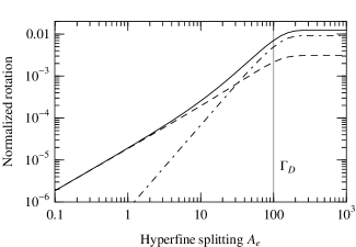
Figure 21: As Fig. 15, but for the wall effect. Parameters are the same as in Fig. 17.

Figure 20 shows the optical rotation spectrum for various values of $A_{e}$, and Fig. 21 shows the maximum of the rotation spectrum as a function of $A_{e}$. These figures can be compared to Figs. 14 and 15 for the Doppler-free transit effect. In particular, we see the same phenomenon of two resonance peaks of the same sign appearing to cancel as they overlap (observation of this effect in anti-relaxation-coated vapor cells is discussed in Ref. Budker et al. (2000b) and in buffer-gas cells in Ref. Novikova et al. (2001)). The explanation for this is the same as in the Doppler-free case. Also as in the Doppler-free case, the rotation is linear in $A_{e}$ to lowest order, and this linear term is due to polarization produced by spontaneous emission:

$$\ell_{0}\frac{d\varphi}{d\ell}=\frac{\sqrt{\pi}}{288}\kappa_{s}x_{1}R\frac{A_{e}\Delta_{1}}{\Gamma_{D}^{2}}e^{-2(\Delta_{1}/\Gamma_{D})^{2}}.$$ (42)

Spectra for the case in which $A_{e}$ and $A_{g}$ are varied together are shown in Fig. 22, and are also similar to the Doppler-free transit effect (Fig. 16).

Figure 22: As Fig. 19, but for the wall effect.

When both $A_{e}$ and $A_{g}$ are small, the signal to lowest order in these quantities is given by

$$\ell_{0}\frac{d\varphi}{d\ell}=A_{e}\left(A_{e}-\frac{R}{3}A_{g}\right)\frac{\kappa_{s}x_{1}\Delta^{2}}{48\,\Gamma_{D}^{4}}e^{-2\Delta^{2}/\Gamma_{D}^{2}}.$$ (43)

III.4 Higher nuclear spin and the $D2$ line

When nuclear spins $I\geq 1/2$ are considered, several complications arise. The clearest of these is that the two ground states now have angular momenta $F_{g}=I\pm\frac{1}{2}\geq 1$, so that they can both support atomic alignment and produce optical rotation. A more subtle difference is that, with higher angular momenta in the excited state, coherences between the excited state hyperfine levels can be created when the excited-state hyperfine splitting is on the order of the natural width or smaller. (Ground-state hyperfine coherences can be neglected as long as the ground-state hyperfine splitting is much larger than the ground-state relaxation rate.) This can change the optical rotation spectrum, and also causes the symmetry between the Doppler-free transit and wall effects discussed above to be partially broken, as we see below.

However, many of the results obtained above for the $I=1/2$ system are a consequence of the general arguments discussed in Sec. II, and thus hold for any nuclear spin. In particular, the dependence of the optical rotation signal on the hyperfine splitting for large ground-state and small excited state splitting [Eqs. (29), (36), and (42)] and for both ground- and excited-state hyperfine splitting small [Eqs. (30), (37), and (43)] remains the same. We have, for large $A_{g}$ and small $A_{e}$, and for a particular transition group, the following three expressions. For the Doppler-free transit effect:

$$\quad\ell_{0}\frac{d\varphi}{d\ell}\propto A_{e}\kappa_{s}x_{F_{g}}R\frac{(\Gamma/2)^{4}\Delta_{F_{g}}}{\big{[}(\Gamma/2)^{2}+\Delta_{F_{g}}^{2}\big{]}^{3}},$$ (44)

for the Doppler-broadened transit effect:

$$\ell_{0}\frac{d\varphi}{d\ell}\propto A_{e}^{2}\kappa_{s}x_{F_{g}}\frac{e^{-\Delta_{F_{g}}^{2}/\Gamma_{D}^{2}}}{\left(\Gamma^{2}+A_{e}^{2}\right)},$$ (45)

and for the wall effect:

$$\ell_{0}\frac{d\varphi}{d\ell}\propto A_{e}\kappa_{s}x_{F_{g}}R\frac{\Delta_{F_{g}}e^{-2(\Delta_{F_{g}}/\Gamma_{D})^{2}}}{\Gamma_{D}^{2}}.$$ (46)

For $A_{g}$ and $A_{e}$ both small, we have, for the Doppler-free transit effect:

$$\ell_{0}\frac{d\varphi}{d\ell}\propto A_{e}\left(A_{e}-\frac{R}{3}A_{g}\right)\frac{\kappa_{s}(\Gamma/2)^{4}\Delta^{2}}{\left[(\Gamma/2)^{2}+\Delta^{2}\right]^{4}},$$ (47)

for the Doppler-broadened effect:

$$\ell_{0}\frac{d\varphi}{d\ell}\propto A_{e}\left(A_{e}-\frac{R}{3}A_{g}\right)\frac{\kappa_{s}}{\Gamma^{2}}e^{-\Delta^{2}/\Gamma_{D}^{2}},$$ (48)

and for the wall effect:

$$\ell_{0}\frac{d\varphi}{d\ell}\propto A_{e}\left(A_{e}-\frac{R}{3}A_{g}\right)\frac{\kappa_{s}\Delta^{2}}{\Gamma_{D}^{4}}e^{-2\Delta^{2}/\Gamma_{D}^{2}}.$$ (49)

To illustrate the differences that arise when the nuclear spin is increased, we plot (analogously to Figs. 15, 17, and 21) in Fig. 23 the maximum of the rotation spectra for large $A_{g}$ as a function of $A_{e}$ for the Doppler-free transit, Doppler-broadened transit, and wall effects. Three values of the nuclear spin are used, $I=1/2$, 3/2, and 5/2, and for $I=3/2$ and 5/2 the rotation on the $F_{g}=I\pm 1/2\rightarrow F_{e}$ lines is plotted separately.

Figure 23: Maximum of the normalized optical rotation spectra $\ell_{0}/(\kappa_{s}x_{F_{g}})d\varphi/d\ell$ for the Doppler-free transit, Doppler-broadened transit, and wall effects on the $D1$ line for $I=1/2$, 3/2, and 5/2. We assume $\Gamma_{D}=100$, $\gamma\ll 1$, $A_{g}\gg\Gamma_{D}$ in units of $\Gamma$. The maxima for the $F_{g}=I\pm 1/2\rightarrow F_{e}$ transitions are plotted separately. Each plot shows rotation due to polarization produced by depopulation (dot-dashed line), rotation due to polarization produced by repopulation (dashed line), and total rotation (solid line). The sharp features seen in some of the plots occur when two terms contributing to the largest resonance cancel. In general, since all resonances are not canceled at the same time, the maximum of the spectrum does not go to zero.

Rotation due to polarization produced by the depopulation and repopulation mechanisms is plotted, as well as the total rotation signal. In many cases these two contributions are of opposite sign, so the details of the total signal can depend on how closely the two contributions cancel each other. (The cancelation tends to be more complete for the $F_{g}=I-1/2$ lines.) However, the qualitative features of these plots follow, in large part, the pattern exhibited in the $I=1/2$ case. One exception is the behavior of the wall effect plot for $A_{e}$ in the neighborhood of the natural width. As mentioned above, when $I>1/2$, excited-state hyperfine coherences can form when the excited-state hyperfine splitting becomes small. This leads to “interference” effects when the Doppler-free resonance lines overlap that do not occur when the Doppler-broadened resonance lines in the wall effect overlap. This breaks the symmetry between the wall effect and the Doppler-free transit effect that is found in the $I=1/2$ case.

We now discuss the $J_{g}=1/2\rightarrow J_{e}=3/2$ $D2$ transition. The presence of three hyperfine levels in the excited state leads to additional features in the dependence of the signal on the hyperfine splitting (Fig. 24).

Figure 24: Maximum of the normalized optical rotation spectra, as in Fig. 23, but for the $D2$ line. For the $I=3/2$, $F_{g}=2$ and the $I=5/2$, $F_{g}=3$ systems for the Doppler-broadened transit effect, the two contributions to optical rotation nearly cancel, with the consequence that the approximations used in obtaining the analytic formulas for the total Doppler-broadened signal begin to break down. Numerical convolution is employed in these cases.

However, the fact that the ground-state electronic momentum is still $J_{g}=1/2$ means that the dependence of the signal on the excited-state hyperfine splitting as $A_{e}$ goes to zero remains the same, for the reasons discussed in Sec. II. Thus, to lowest order in $A_{e}$, the rotation signals on the $D2$ line for large $A_{g}$ are given by Eqs. (44–46). (We set the hyperfine coefficient $B_{e}$ to zero for simplicity.)

Considering the signals obtained when both the excited- and ground-state hyperfine splittings are small, we expect somewhat different behavior for the contribution due to polarization produced by repopulation pumping than in the $D1$ case. This is because the excited-state electronic angular momentum is $J_{e}=3/2$, so that production of rank $\kappa=2<2J_{e}$ atomic alignment in the ground-state by spontaneous emission is allowed even when the ground-state hfs is unresolved (Sec. II.2). The lowest order dependence on hyperfine splitting for the $D2$ line is given by

$$\ell_{0}\frac{d\varphi}{d\ell}\propto A_{e}\left[A_{e}-R\left(2A_{e}+\frac{1}{3}A_{g}\right)\right]$$ (50)

for each of the three effects, with the spectral line shapes remaining as in Eqs. (47–49). Note that there is now a term that depends on polarization due to repopulation that does not go to zero as $A_{g}$ goes to zero.

III.5 The alkalis

We now examine the consequences of the preceding discussion for the alkali atoms commonly used in nonlinear magneto-optical experiments. In Fig. 25 the maximum of the spectrum of optical rotation is plotted for the D1 and D2 lines of several alkali atoms.

Figure 25: Maximum of the spectrum of normalized optical rotation for the (a) Doppler-broadened transit effect and (b) wall effect for various alkali atoms. Circles indicate the D1 line and triangles indicate the D2 line. Room temperature Maxwellian velocity distributions are assumed. Normalized rotation is defined here as $\ell_{0}/(\kappa_{s}x_{I+J_{g}})(d\varphi/d\ell)$, where $\ell_{0}$ in this case is the unsaturated absorption length at the detuning that gives maximum absorption. The normalized magnitude of unsuppressed optical rotation is nominally on the order of unity; however, this is to some degree dependent on the normalization convention chosen. For example, if the maximum matrix element of $d_{z}$ is used in the definition of $\kappa_{s}$, rather than the reduced matrix element, the values in this plot are increased by a factor of $\sim\!6$.

The Doppler-broadened transit effect is shown in Fig. 25a and the wall effect is shown in Fig. 25b. (Numerical convolution was used to obtain these results, because the alkalis do not all satisfy the conditions under which the analytic formulas were derived.) The nuclear spins, hyperfine splittings, excited state lifetimes, and Doppler widths all vary between the different alkali atoms. However, focusing our attention on the hyperfine splittings, which have the greatest degree of variation, we can see the correspondence of these results to the preceding discussion. In particular, we have seen that the magnitude of the Doppler-broadened transit effect is largely independent of the hyperfine splitting when the splittings are greater than the natural width of the transition. This is generally the case for the alkalis, leading to the relative constancy of the magnitude of the transit effect among the alkalis. For the wall effect, on the other hand, we have found that the magnitude of the effect diminishes when the hyperfine splitting becomes less than the Doppler width. In the alkalis the excited state hyperfine splitting is generally on the order of or smaller than the Doppler width, and the general trend is that the ratio of hyperfine splitting to Doppler width increases as the atomic mass number increases. This accounts for the general upward trend in Fig. 25b. The trend is not completely consistent: the hyperfine splitting of K is smaller than that of Na, which is reflected in the plot of the wall effect.

IV Conclusion

In experiments involving light-induced polarization in the alkali atoms, the effect of partially resolved hyperfine structure is of practical importance. We have addressed this question from both descriptive and quantitative standpoints. We have formulated rules describing various restrictions on the rank of atomic polarization moments that can be created or detected by light in cases when either the ground- or excited-state hyperfine structure is completely unresolved. We have also studied the particular situation of nonlinear Faraday rotation under various experimental conditions in more generality, and presented analytic formulas giving the results of optical rotation measurements when the hfs is unresolved, partially resolved, or completely resolved.

Appendix A Nonlinear magneto-optical rotation with hyperfine structure

A.1 Perturbation theory with polarization moments

The time evolution of the atomic density matrix $\rho$ under the action of a time-independent Hamiltonian $H$ is given by the Liouville equation, which can be derived from the Schrödinger equation (with phenomenological relaxation terms added by hand). Setting $\hbar=c=1$, the Liouville equation can be written

$$\dot{\rho}=-i\left[H,\rho\right]-\frac{1}{2}\left\{\Gamma,\rho\right\}+\Lambda+\operatorname{Tr}\left(\mathcal{F}\rho\right),$$ (51)

where the square brackets denote the commutator and the curly brackets the anticommutator, $\Gamma$ is a Hermitian relaxation matrix that accounts for relaxation mechanisms such as transit relaxation due to atoms leaving the region of interest and intrinsic relaxation of excited states due to spontaneous emission, $\Lambda$ accounts for repopulation mechanisms, such as transit repopulation, that do not depend on $\rho$, and $\mathcal{F}$ is the spontaneous emission operator, accounting for repopulation of ground states due to spontaneous emission from excited states. (We neglect other relaxation and repopulation mechanisms, such as spin-exchanging collisions, which may require the inclusion of additional terms). The spontaneous emission operator, defined by Barrat and Cohen-Tannoudji (1961a, b)

$$\mathcal{F}^{sr}_{mn}=\frac{4}{3}\omega_{rm}^{3}{\boldsymbol{{\mathbf{d}}}}_{mr}\cdot{\boldsymbol{{\mathbf{d}}}}_{sn},$$ (52)

connects a pair of excited states ${|s\rangle}$, ${|r\rangle}$ to a pair of ground states ${|m\rangle}$, ${|n\rangle}$; the trace in Eq. 51 is taken over the excited state pair.

We can expand the operators appearing in the Liouville equation in terms of the polarization operators $T^{(\kappa)}_{q}(F_{1}F_{2})$ according to

$$A=\sum A^{(\kappa q)}(F_{1}F_{2})T^{(\kappa)}_{q}(F_{1}F_{2}),$$ (53)

where $F_{1,2}$ runs over all pairs of states in the system. (Here $F$ is understood to represent the total angular momentum quantum number as well as any additional quantum numbers necessary to distinguish between two states with the same total angular momentum.) The expansion coefficients $A^{(\kappa q)}(F_{1}F_{2})$ can be found from the Wigner-Eckart theorem, along with the orthonormality condition

$$\operatorname{Tr}\left(T^{(\kappa)}_{q}(F_{1}F_{2})\left(T^{(\kappa^{\prime})}_{q^{\prime}}(F_{1}^{\prime}F_{2}^{\prime})\right)^{\dagger}\right)=\delta_{\kappa\kappa^{\prime}}\delta_{qq^{\prime}}\delta_{F_{1}F_{1}^{\prime}}\delta_{F_{2}F_{2}^{\prime}}$$ (54)

and the phase convention

$$\begin{split}\left(T^{(\kappa)}_{q}(F_{1}F_{2})\right)^{\dagger}&=(-1)^{F_{1}-F_{2}+q}T^{(\kappa)}_{-q}(F_{2}F_{1})\\ &=T^{(\kappa q)}(F_{1}F_{2}).\end{split}$$ (55)

There are several equivalent expressions for the expansion coefficients; one such form is

$$\begin{split}A^{(\kappa q)}(F_{1}F_{2})&=\sum_{mm^{\prime}}(-1)^{F_{1}-F_{2}+q}\sqrt{\frac{2\kappa+1}{2F_{2}+1}}{\langle F_{1}m\kappa,-q|F_{2}m^{\prime}\rangle}A_{F_{1}m,F_{2}m^{\prime}}.\\ \end{split}$$ (56)

The set of expansion coefficients for the density matrix are known as polarization moments. Performing the expansion of each operator, and using appropriate tensor product and sum rules, the equation of motion for the polarization moments is found from the Liouville equation to be

$$\begin{split}\dot{\rho}^{(\kappa q)}(F_{1}F_{2})=&-i(-1)^{F_{1}+F_{2}+\kappa}\sum\sqrt{(2\kappa^{\prime}+1)(2\kappa^{\prime\prime}+1)}{\langle\kappa^{\prime}q^{\prime}\kappa^{\prime\prime}q^{\prime\prime}|\kappa q\rangle}\begin{Bmatrix}\kappa^{\prime}&\kappa^{\prime\prime}&\kappa\\ F_{2}&F_{1}&F_{3}\end{Bmatrix}\\ &\qquad\qquad\times\Bigg{[}\left(H^{(\kappa^{\prime}q^{\prime})}(F_{1}F_{3})-\frac{i}{2}\Gamma^{(\kappa^{\prime}q^{\prime})}(F_{1}F_{3})\right)\rho^{(\kappa^{\prime\prime}q^{\prime\prime})}(F_{3}F_{2})\\ &\qquad\qquad\qquad\qquad-\rho^{(\kappa^{\prime}q^{\prime})}(F_{1}F_{3})\left(H^{(\kappa^{\prime\prime}q^{\prime\prime})}(F_{3}F_{2})+\frac{i}{2}\Gamma^{(\kappa^{\prime\prime}q^{\prime\prime})}(F_{3}F_{2})\right)\Bigg{]}\\ &+\Lambda^{(\kappa q)}(F_{1}F_{2})+\frac{4}{3}\omega_{0}^{3}\sum(F_{1}\|d\|F_{e})\rho^{(\kappa q)}(F_{e}F_{e}^{\prime})(F_{e}^{\prime}\|d\|F_{2})(-1)^{F_{e}+F_{e}^{\prime}+\kappa+1}\begin{Bmatrix}\kappa&F_{2}&F_{1}\\ 1&F_{e}&F_{e}^{\prime}\end{Bmatrix},\end{split}$$ (57)

where all variables not appearing on the left-hand side are summed over (the variables $F_{e}$ and $F_{e}^{\prime}$ appearing in the last term relate to spontaneous emission and run over only those states of higher energy than $F_{1,2}$). Here the arrays enclosed in in curly brackets are the $6j$ symbols.

We now suppose that the total Hamiltonian $H=H_{0}+V$, where $H_{0}$ is diagonal and $V$ is a time-independent perturbation. We also assume that $\Gamma$ and $\Lambda$ are diagonal. More precisely, we assume that only $\Gamma^{(00)}(FF)$, $\Lambda^{(00)}(FF)$, and $H^{(00)}(FF)$ are nonzero (for arbitrary $F$). Taking the steady-state limit in Eq. (57) and expanding to second order in the perturbation $V$, we find for a ground-state polarization moment

$$\begin{split}\rho^{(\kappa q)}(F_{g}F_{g})&=\frac{\gamma}{i\widetilde{\omega}_{FF}N_{g}}\Bigg{[}\delta_{\kappa 0}\delta_{q0}\sqrt{2F_{g}+1}-(-1)^{2F_{g}+\kappa^{\prime}+\kappa^{\prime\prime}}\sqrt{(2\kappa^{\prime}+1)(2\kappa^{\prime\prime}+1)}{\langle\kappa^{\prime}q^{\prime}\kappa^{\prime\prime}q^{\prime\prime}|\kappa q\rangle}\\ &\qquad\qquad\qquad\times\begin{Bmatrix}\kappa^{\prime\prime}&\kappa^{\prime}&\kappa\\ F_{g}&F_{g}&F^{\prime}\end{Bmatrix}\frac{\widetilde{\omega}_{F_{g}F^{\prime}}+\widetilde{\omega}_{F^{\prime}F_{g}}}{\widetilde{\omega}_{F_{g}F_{g}}\widetilde{\omega}_{F_{g}F^{\prime}}\widetilde{\omega}_{F^{\prime}F_{g}}}V^{(\kappa^{\prime}q^{\prime})}(F^{\prime}F_{g})V^{(\kappa^{\prime\prime}q^{\prime\prime})}(F_{g}F^{\prime})\\ &\qquad\qquad-i\frac{4}{3}\omega_{0}(-1)^{2F^{\prime}_{1}+2F^{\prime}_{2}+\kappa+\kappa^{\prime}+\kappa^{\prime\prime}}\sqrt{(2\kappa^{\prime}+1)(2\kappa^{\prime\prime}+1)}{\langle\kappa^{\prime}q^{\prime}\kappa^{\prime\prime}q^{\prime\prime}|\kappa q\rangle}\begin{Bmatrix}\kappa^{\prime\prime}&\kappa^{\prime}&\kappa\\ F^{\prime}_{2}&F^{\prime}_{1}&F^{\prime}\end{Bmatrix}\begin{Bmatrix}\kappa&F_{g}&F_{g}\\ 1&F^{\prime}_{1}&F^{\prime}_{2}\end{Bmatrix}\\ &\qquad\qquad\qquad\times(F^{\prime}_{2}\|d\|F_{g})(F_{g}\|d\|F^{\prime}_{1})\frac{\widetilde{\omega}_{F^{\prime}_{1}F^{\prime}}+\widetilde{\omega}_{F^{\prime}F^{\prime}_{2}}}{\widetilde{\omega}_{F^{\prime}_{1}F^{\prime}}\widetilde{\omega}_{F^{\prime}_{1}F^{\prime}_{2}}\widetilde{\omega}_{F^{\prime}F^{\prime}}\widetilde{\omega}_{F^{\prime}F^{\prime}_{2}}}V^{(\kappa^{\prime\prime}q^{\prime\prime})}(F^{\prime}_{1}F^{\prime})V^{(\kappa^{\prime}q^{\prime})}(F^{\prime}F^{\prime}_{2})\Bigg{]}.\end{split}$$ (58)

Here we have neglected the possibility of cascade decays and assumed that $V$ does not couple a state to itself. We also have assumed that $\Lambda$ repopulates all ground-state sublevels equally; i.e. $\Lambda_{Fm,Fm}=\gamma/N_{g}$, where $\gamma$ is the ground-state relaxation rate and $N_{g}$ is the total number of ground-state sublevels. The complex energy splitting $\widetilde{\omega}_{F_{1}F_{2}}$ is given by

$$\begin{split}\widetilde{\omega}_{F_{1}F_{2}}=E_{F_{1}}-E_{F_{2}}-\frac{i}{2}\left(\Gamma_{F_{1}}+\Gamma_{F_{2}}\right),\end{split}$$ (59)

where $E_{F}=(2F+1)^{-1/2}H_{0}^{(00)}(FF)$ is the unperturbed energy and $\Gamma_{F}=(2F+1)^{-1/2}\Gamma^{(00)}(FF)$ is the total relaxation rate of a state $F$.

A.2 Doppler-free transit effect

We now apply the results obtained in Sec. A.1 to the three-stage calculation described in Sec. III.1. In stage (a), we consider a ${\boldsymbol{{\mathbf{\hat{z}}}}}$-polarized optical electric field ${\boldsymbol{{\mathbf{\mathcal{E}}}}}=\mathcal{E}_{0}\operatorname{Re}\left({\boldsymbol{{\mathbf{\hat{e}}}}}e^{i({\boldsymbol{{\mathbf{k}}}}\cdot{\boldsymbol{{\mathbf{r}}}}-\omega t)}\right)$, where $\mathcal{E}_{0}$ is the optical electric field amplitude, ${\boldsymbol{{\mathbf{\hat{e}}}}}={\boldsymbol{{\mathbf{\hat{z}}}}}$ is the polarization vector, ${\boldsymbol{{\mathbf{\hat{k}}}}}={\boldsymbol{{\mathbf{\hat{x}}}}}$ is the wave vector, and $\omega$ is the optical frequency. We let $V$ represent the electric-dipole Hamiltonian in the rotating-wave approximation: $V^{\prime}=-\frac{1}{2}d_{z}\mathcal{E}_{0}$. (Here the prime refers to the rotating frame.) We assume that the magnetic field is absent in this stage. From Eq. (58) we find

$$\begin{split}\rho_{a}^{(20)}(F_{g}F_{g})&=-\sqrt{\frac{2}{3}}\sum_{F_{e}}(-1)^{F_{g}-F_{e}}\kappa_{s}\frac{(2F_{e}+1)(2F_{g}+1)}{(2I+1)(2J_{g}+1)}\Bigg{(}(-1)^{2I+2J_{g}}\begin{Bmatrix}1&1&2\\ F_{g}&F_{g}&F_{e}\end{Bmatrix}\begin{Bmatrix}J_{e}&F_{e}&I\\ F_{g}&J_{g}&1\end{Bmatrix}^{2}L(\omega^{\prime}_{F_{e}F_{g}})\\ &\qquad\qquad+R\sum_{F_{g}^{\prime}F_{e}^{\prime}}(-1)^{F_{g}^{\prime}-F_{e}^{\prime}}(2J_{e}+1)(2F_{g}^{\prime}+1)(2F_{e}^{\prime}+1)\begin{Bmatrix}1&1&2\\ F_{e}&F_{e}^{\prime}&F_{g}^{\prime}\end{Bmatrix}\begin{Bmatrix}F_{g}&F_{g}&2\\ F_{e}&F_{e}^{\prime}&1\end{Bmatrix}\\ &\qquad\qquad\qquad\times\begin{Bmatrix}J_{e}&F_{e}&I\\ F_{g}&J_{g}&1\end{Bmatrix}\begin{Bmatrix}J_{e}&F_{e}&I\\ F_{g}^{\prime}&J_{g}&1\end{Bmatrix}\begin{Bmatrix}J_{e}&F_{e}^{\prime}&I\\ F_{g}&J_{g}&1\end{Bmatrix}\begin{Bmatrix}J_{e}&F_{e}^{\prime}&I\\ F_{g}^{\prime}&J_{g}&1\end{Bmatrix}\frac{L(\omega^{\prime}_{F_{e}F_{g}^{\prime}})L(\omega^{\prime}_{F_{e}^{\prime}F_{g}^{\prime}})}{L\!\left(\sqrt{\vphantom{y}\smash[b]{\omega^{\prime}_{F_{e}F_{g}^{\prime}}\omega^{\prime}_{F_{e}^{\prime}F_{g}^{\prime}}}}\right)}\Bigg{)},\end{split}$$ (60)

where all variables are as defined in Sec. III.1. We have evaluated matrix elements using the Wigner-Eckart theorem and have used the relation (see, for example, Ref. Sobelman (1992))

$$R\,\Gamma=\frac{4}{3}\frac{\omega^{3}}{2J_{e}+1}(J_{g}\|d\|J_{e})^{2}.$$ (61)

The unperturbed energies can be evaluated with

$$\begin{split}E_{JFM}&=E_{J}+\frac{1}{2}K_{IJF}A_{J}\\ &+\frac{3}{8}\frac{K_{IJF}(K_{IJF}+1)-\frac{4}{3}I(I+1)J(J+1)}{I(2I-1)J(2J-1)}B_{J},\end{split}$$ (62)

where $K_{IJF}=F(F+1)-I(I+1)-J(J+1)$ and $A_{J}$ and $B_{J}$ are the hyperfine coefficients. The last term is zero for $J\leq 1/2$ or $I\leq 1/2$.

In the case in which the excited-state hfs is well resolved in the Doppler-free spectrum ($\omega_{F_{e}F_{e}^{\prime}}\gg\Gamma$), Eq. (60) reduces to

$$\begin{split}&\rho_{a}^{(20)}(F_{g}F_{g})=-\sqrt{\frac{2}{3}}\sum_{F_{e}}(-1)^{F_{g}-F_{e}}\kappa_{s}\frac{(2F_{e}+1)(2F_{g}+1)}{(2I+1)(2J_{g}+1)}\Bigg{(}(-1)^{2I+2J_{g}}\begin{Bmatrix}1&1&2\\ F_{g}&F_{g}&F_{e}\end{Bmatrix}\begin{Bmatrix}J_{e}&F_{e}&I\\ F_{g}&J_{g}&1\end{Bmatrix}^{2}L(\omega^{\prime}_{F_{e}F_{g}})\\ &\quad+\sum_{F_{g}^{\prime}}R\,(-1)^{F_{g}^{\prime}-F_{e}}(2J_{e}+1)(2F_{g}^{\prime}+1)(2F_{e}+1)\begin{Bmatrix}1&1&2\\ F_{e}&F_{e}&F_{g}^{\prime}\end{Bmatrix}\begin{Bmatrix}F_{g}&F_{g}&2\\ F_{e}&F_{e}&1\end{Bmatrix}\begin{Bmatrix}J_{e}&F_{e}&I\\ F_{g}&J_{g}&1\end{Bmatrix}^{2}\begin{Bmatrix}J_{e}&F_{e}&I\\ F_{g}^{\prime}&J_{g}&1\end{Bmatrix}^{2}L(\omega^{\prime}_{F_{e}F_{g}^{\prime}})\Bigg{)}.\\ \end{split}$$ (63)

In stage (b), the ground-state density matrix, which is initially in the state found in stage (a), evolves under the influence of a magnetic field $B{\boldsymbol{{\mathbf{\hat{x}}}}}$. We will require only the value of the polarization moment $\rho_{b}^{(21)}(F_{g}F_{g})$. Using the Hamiltonian $H_{B}=-{\boldsymbol{{\mathbf{\mu}}}}\cdot{\boldsymbol{{\mathbf{B}}}}$ in Eq. (57) and solving for the steady state, we find

$$\begin{split}\rho_{b}^{(21)}(F_{g}F_{g})=i\frac{\sqrt{3}}{2\sqrt{2}}x_{F_{g}}\rho_{a}^{(20)}(F_{g}F_{g}).\end{split}$$ (64)

where the magnetic-resonance line-shape parameter $x_{F_{g}}$ is defined in Eq. (27).

In stage (c) the ground-state polarization is probed. The effect of the atoms on the light polarization as the light traverses the atomic medium can be found in terms of coherences between ground and excited states using the wave equation:

$$\frac{\partial{\boldsymbol{{\mathbf{\mathcal{E}}}}}}{\partial\ell^{2}}-\frac{\partial{\boldsymbol{{\mathbf{\mathcal{E}}}}}}{\partial t^{2}}=4\pi\frac{\partial{\boldsymbol{{\mathbf{P}}}}}{\partial t^{2}},$$ (65)

where $\ell$ is the distance along the light propagation direction, and ${\boldsymbol{{\mathbf{P}}}}=n\operatorname{Tr}\rho{\boldsymbol{{\mathbf{d}}}}$ is the medium dipole polarization ($n$ is atomic density), which can be written in terms of the rotating-frame density matrix $\rho^{\prime}$ as

$$\begin{split}{\boldsymbol{{\mathbf{P}}}}=n\sum_{mp}2\operatorname{Re}\left(\rho^{\prime}_{pm}{\boldsymbol{{\mathbf{d}}}}_{mp}e^{i({\boldsymbol{{\mathbf{k}}}}\cdot{\boldsymbol{{\mathbf{r}}}}-\omega t)}\right),\end{split}$$ (66)

where $m$ runs over ground states, and $p$ runs over excited states. Using the parameterization of a general optical electric field in terms of the polarization angle $\varphi$ and ellipticity $\epsilon$,

$$\begin{split}{\boldsymbol{{\mathbf{\mathcal{E}}}}}&=\mathcal{E}_{0}\operatorname{Re}\Big{(}e^{i({\boldsymbol{{\mathbf{k}}}}\cdot{\boldsymbol{{\mathbf{r}}}}-\omega t+\phi)}[\left(\cos\varphi\cos\epsilon-i\sin\varphi\sin\epsilon\right){\boldsymbol{{\mathbf{\hat{e}}}}}_{1}\\ &\qquad\qquad{}+\left(\sin\varphi\cos\epsilon+i\cos\varphi\sin\epsilon\right){\boldsymbol{{\mathbf{\hat{e}}}}}_{2}]\Big{)},\end{split}$$ (67)

where ${\boldsymbol{{\mathbf{\hat{e}}}}}_{1,2}$ are orthogonal transverse unit vectors, we obtain for optical rotation in the case of linear polarization

$$\begin{split}\frac{d\varphi}{d\ell}&=-\frac{4\pi\omega n}{\mathcal{E}_{0}}\sum\operatorname{Im}\left[\rho^{\prime}_{pm}{\boldsymbol{{\mathbf{d}}}}_{mp}\cdot({\boldsymbol{{\mathbf{\hat{k}}}}}\times{\boldsymbol{{\mathbf{\hat{e}}}}})\right].\end{split}$$ (68)

Using first-order perturbation theory for the optical coherences and neglecting coherences between nondegenerate ground states, we obtain the optical rotation for weak probe light in terms of the ground-state density matrix:

$$\frac{d\varphi}{d\ell}=-2\pi\omega n\operatorname{Im}\left[{\boldsymbol{{\mathbf{\hat{e}}}}}\cdot\beta\cdot({\boldsymbol{{\mathbf{\hat{k}}}}}\times{\boldsymbol{{\mathbf{\hat{e}}}}})\right],$$ (69)

where we have defined

$$\begin{split}\beta&=\sum_{pmn}\frac{{\boldsymbol{{\mathbf{d}}}}_{pn}\rho_{nm}{\boldsymbol{{\mathbf{d}}}}_{mp}}{\widetilde{\omega}_{pm}^{\prime}}.\end{split}$$ (70)

Expanding the tensor $\beta$ in terms of the ground-state polarization moments, we obtain

$$\begin{split}\beta&=\sum_{F_{g}F_{e}\kappa q^{\prime}q^{\prime\prime}}\frac{(-1)^{F_{g}+F_{e}+\kappa}}{\widetilde{\omega}_{F_{e}F_{g}}^{\prime}}{\boldsymbol{{\mathbf{\hat{\epsilon}}}}}_{-q^{\prime}}{\boldsymbol{{\mathbf{\hat{\epsilon}}}}}_{-q^{\prime\prime}}{\langle 1q^{\prime}1q^{\prime\prime}|\kappa,q^{\prime}+q^{\prime\prime}\rangle}\begin{Bmatrix}1&1&\kappa\\ F_{g}&F_{g}&F_{e}\end{Bmatrix}\left|(F_{g}\|d\|F_{e})\right|^{2}\rho^{(\kappa,q^{\prime}+q^{\prime\prime})}(F_{g}F_{g}),\end{split}$$ (71)

where ${\boldsymbol{{\mathbf{\hat{\epsilon}}}}}_{q}$ are the spherical basis vectors.

Evaluating (69) for our case and using Eq. (64) gives

$$\begin{split}\ell_{0}\frac{d\varphi}{d\ell}&=-\frac{3\sqrt{3}}{4\sqrt{2}}\sum_{F_{g}F_{e}}(-1)^{F_{g}+F_{e}}(2F_{g}+1)(2F_{e}+1)(2J_{g}+1)\begin{Bmatrix}1&1&2\\ F_{g}&F_{g}&F_{e}\end{Bmatrix}\begin{Bmatrix}J_{e}&F_{e}&I\\ F_{g}&J_{g}&1\end{Bmatrix}^{2}L(\omega_{F_{e}F_{g}}^{\prime})x_{F_{g}}\rho_{a}^{(20)}(F_{g}F_{g}),\end{split}$$ (72)

where the unsaturated absorption length for the $J_{g}\rightarrow J_{e}$ transition is defined in Eq. (28). Substituting in Eq. (60) results in the complete expression for optical rotation for the Doppler-free transit effect:

$$\begin{split}\ell_{0}\frac{d\varphi}{d\ell}&=\frac{3}{4}\kappa_{s}\sum_{F_{g}F_{e}F_{e}^{\prime\prime}}(-1)^{2F_{g}+F_{e}^{\prime\prime}-F_{e}}\frac{(2F_{e}+1)(2F_{e}^{\prime\prime}+1)(2F_{g}+1)^{2}}{(2I+1)}\begin{Bmatrix}1&1&2\\ F_{g}&F_{g}&F_{e}^{\prime\prime}\end{Bmatrix}\begin{Bmatrix}J_{e}&F_{e}^{\prime\prime}&I\\ F_{g}&J_{g}&1\end{Bmatrix}^{2}x_{F_{g}}\\ &\qquad\times\Bigg{(}(-1)^{2I+2J_{g}}\begin{Bmatrix}1&1&2\\ F_{g}&F_{g}&F_{e}\end{Bmatrix}\begin{Bmatrix}J_{e}&F_{e}&I\\ F_{g}&J_{g}&1\end{Bmatrix}^{2}L(\omega^{\prime}_{F_{e}F_{g}})L(\omega_{F_{e}^{\prime\prime}F_{g}}^{\prime})\\ &\qquad\qquad+R\sum_{F_{g}^{\prime}F_{e}^{\prime}}(-1)^{F_{g}^{\prime}-F_{e}^{\prime}}(2J_{e}+1)(2F_{g}^{\prime}+1)(2F_{e}^{\prime}+1)\begin{Bmatrix}1&1&2\\ F_{e}&F_{e}^{\prime}&F_{g}^{\prime}\end{Bmatrix}\begin{Bmatrix}F_{g}&F_{g}&2\\ F_{e}&F_{e}^{\prime}&1\end{Bmatrix}\\ &\qquad\qquad\qquad\times\begin{Bmatrix}J_{e}&F_{e}&I\\ F_{g}&J_{g}&1\end{Bmatrix}\begin{Bmatrix}J_{e}&F_{e}&I\\ F_{g}^{\prime}&J_{g}&1\end{Bmatrix}\begin{Bmatrix}J_{e}&F_{e}^{\prime}&I\\ F_{g}&J_{g}&1\end{Bmatrix}\begin{Bmatrix}J_{e}&F_{e}^{\prime}&I\\ F_{g}^{\prime}&J_{g}&1\end{Bmatrix}\frac{L(\omega^{\prime}_{F_{e}F_{g}^{\prime}})L(\omega^{\prime}_{F_{e}^{\prime}F_{g}^{\prime}})L(\omega_{F_{e}^{\prime\prime}F_{g}}^{\prime})}{L\!\left(\sqrt{\vphantom{y}\smash[b]{\omega^{\prime}_{F_{e}F_{g}^{\prime}}\omega^{\prime}_{F_{e}^{\prime}F_{g}^{\prime}}}}\right)}\Bigg{)}.\end{split}$$ (73)

For completely resolved hfs ($\omega_{F_{e}F_{e}^{\prime}},\omega_{F_{g}F_{g}^{\prime}}\gg\Gamma$), this reduces to

$$\begin{split}\ell_{0}\frac{d\varphi}{d\ell}&=\frac{3}{4}\kappa_{s}\sum_{F_{g}F_{e}}(-1)^{2F_{g}}\frac{(2F_{e}+1)^{3}(2F_{g}+1)^{3}}{(2I+1)}\begin{Bmatrix}1&1&2\\ F_{g}&F_{g}&F_{e}\end{Bmatrix}\begin{Bmatrix}J_{e}&F_{e}&I\\ F_{g}&J_{g}&1\end{Bmatrix}^{4}x_{F_{g}}\left[L(\omega_{F_{e}F_{g}}^{\prime})\right]^{2}\\ &\times\Bigg{(}\frac{(-1)^{2I+2J_{g}}}{(2F_{e}+1)(2F_{g}+1)}\begin{Bmatrix}1&1&2\\ F_{g}&F_{g}&F_{e}\end{Bmatrix}+R\,(-1)^{F_{g}-F_{e}}(2J_{e}+1)\begin{Bmatrix}1&1&2\\ F_{e}&F_{e}&F_{g}\end{Bmatrix}\begin{Bmatrix}F_{g}&F_{g}&2\\ F_{e}&F_{e}&1\end{Bmatrix}\begin{Bmatrix}J_{e}&F_{e}&I\\ F_{g}&J_{g}&1\end{Bmatrix}^{2}\Bigg{)}.\end{split}$$ (74)

A.3 Doppler-broadened transit effect

The procedure used to obtain the optical rotation signal in the Doppler-broadened case is described in Sec. III.2. When the ground- and excited-state hyperfine splittings are all much greater than the natural width ($\omega_{F_{e}F_{e}^{\prime}},\omega_{F_{g}F_{g}^{\prime}},\Gamma_{D}\gg\Gamma$) we have, applying the integration procedure to Eq. (74),

$$\begin{split}\ell_{0}\frac{d\varphi}{d\ell}&=\frac{3}{8}\kappa_{s}\sum_{F_{g}F_{e}}(-1)^{2F_{g}}\frac{(2F_{e}+1)^{3}(2F_{g}+1)^{3}}{(2I+1)}\begin{Bmatrix}1&1&2\\ F_{g}&F_{g}&F_{e}\end{Bmatrix}\begin{Bmatrix}J_{e}&F_{e}&I\\ F_{g}&J_{g}&1\end{Bmatrix}^{4}e^{-(\Delta_{F_{e}F_{g}}/\Gamma_{D})^{2}}x_{F_{g}}\\ &\times\Bigg{(}\frac{(-1)^{2I+2J_{g}}}{(2F_{e}+1)(2F_{g}+1)}\begin{Bmatrix}1&1&2\\ F_{g}&F_{g}&F_{e}\end{Bmatrix}+R\,(-1)^{F_{g}-F_{e}}(2J_{e}+1)\begin{Bmatrix}1&1&2\\ F_{e}&F_{e}&F_{g}\end{Bmatrix}\begin{Bmatrix}F_{g}&F_{g}&2\\ F_{e}&F_{e}&1\end{Bmatrix}\begin{Bmatrix}J_{e}&F_{e}&I\\ F_{g}&J_{g}&1\end{Bmatrix}^{2}\Bigg{)},\end{split}$$ (75)

where the unsaturated absorption length for the Doppler-broadened case is given by Eq. (35).

In another limit in which the ground-state hyperfine splittings are much greater than the natural width and the excited-state splittings are much less than the Doppler width ($\omega_{F_{e}F_{e}^{\prime}},\Gamma\ll\Gamma_{D}$, $\Gamma\ll\omega_{F_{g}F_{g}^{\prime}}$), we have

$$\begin{split}\ell_{0}\frac{d\varphi}{d\ell}&=\frac{3}{8}\kappa_{s}\sum_{F_{g}F_{e}F_{e}^{\prime\prime}}(-1)^{2F_{g}+F_{e}^{\prime\prime}-F_{e}}\frac{(2F_{e}+1)(2F_{e}^{\prime\prime}+1)(2F_{g}+1)^{2}}{(2I+1)}\begin{Bmatrix}1&1&2\\ F_{g}&F_{g}&F_{e}^{\prime\prime}\end{Bmatrix}\begin{Bmatrix}J_{e}&F_{e}&I\\ F_{g}&J_{g}&1\end{Bmatrix}^{2}\begin{Bmatrix}J_{e}&F_{e}^{\prime\prime}&I\\ F_{g}&J_{g}&1\end{Bmatrix}^{2}x_{F_{g}}\\ &\qquad\times\Bigg{(}(-1)^{2I+2J_{g}}\begin{Bmatrix}1&1&2\\ F_{g}&F_{g}&F_{e}\end{Bmatrix}+R\sum_{F_{e}^{\prime}}(-1)^{F_{g}-F_{e}^{\prime}}(2J_{e}+1)(2F_{g}+1)(2F_{e}^{\prime}+1)\begin{Bmatrix}1&1&2\\ F_{e}&F_{e}^{\prime}&F_{g}\end{Bmatrix}\begin{Bmatrix}F_{g}&F_{g}&2\\ F_{e}&F_{e}^{\prime}&1\end{Bmatrix}\\ &\qquad\qquad\qquad\qquad\qquad\qquad\times\begin{Bmatrix}J_{e}&F_{e}^{\prime}&I\\ F_{g}&J_{g}&1\end{Bmatrix}^{2}\frac{\left[2\Gamma^{4}+(2\Gamma^{2}+\omega^{2}_{F_{e}F_{e}^{\prime}})\omega_{F_{e}F_{e}^{\prime\prime}}\omega_{F_{e}^{\prime}F_{e}^{\prime\prime}}\right]}{2(\Gamma^{2}+\omega^{2}_{F_{e}F_{e}^{\prime}})(\Gamma^{2}+\omega^{2}_{F_{e}^{\prime}F_{e}^{\prime\prime}})}\Bigg{)}\frac{e^{-(\Delta_{F_{g}}/\Gamma_{D})^{2}}\Gamma^{2}}{\Gamma^{2}+\omega^{2}_{F_{e}F_{e}^{\prime\prime}}}.\end{split}$$ (76)

A.4 Wall effect

The procedure for obtaining the signal in the wall effect case is described in Sec. III.3. For excited-state hyperfine splittings much greater than the natural width ($\Gamma\ll\omega_{F_{e}F_{e}^{\prime}},\Gamma_{D}$), we have for the ground-state polarization

$$\begin{split}\rho_{a}^{(20)}(F_{g}F_{g})&=-\sqrt{\frac{\pi}{6}}\sum_{F_{e}}(-1)^{F_{g}-F_{e}}\kappa_{s}\frac{(2F_{e}+1)(2F_{g}+1)}{(2I+1)(2J_{g}+1)}\begin{Bmatrix}J_{e}&F_{e}&I\\ F_{g}&J_{g}&1\end{Bmatrix}^{2}\Bigg{(}(-1)^{2I+2J_{g}}\begin{Bmatrix}1&1&2\\ F_{g}&F_{g}&F_{e}\end{Bmatrix}e^{-(\Delta_{F_{e}F_{g}}/\Gamma_{D})^{2}}\\ &\qquad\qquad+R\sum_{F_{g}^{\prime}}(-1)^{F_{g}^{\prime}-F_{e}}(2J_{e}+1)(2F_{g}^{\prime}+1)(2F_{e}+1)\begin{Bmatrix}1&1&2\\ F_{e}&F_{e}&F_{g}^{\prime}\end{Bmatrix}\begin{Bmatrix}F_{g}&F_{g}&2\\ F_{e}&F_{e}&1\end{Bmatrix}\begin{Bmatrix}J_{e}&F_{e}&I\\ F_{g}^{\prime}&J_{g}&1\end{Bmatrix}^{2}\Bigg{)},\end{split}$$ (77)

where the saturation parameter for the wall effect is defined by Eq. (40). The optical rotation signal is then given by

$$\begin{split}\ell_{0}\frac{d\varphi}{d\ell}&=-\frac{3\sqrt{3}}{4\sqrt{2}}\sum_{F_{g}F_{e}^{\prime}}(-1)^{F_{g}+F_{e}^{\prime}}(2F_{g}+1)(2F_{e}^{\prime}+1)(2J_{g}+1)\begin{Bmatrix}1&1&2\\ F_{g}&F_{g}&F_{e}^{\prime}\end{Bmatrix}\begin{Bmatrix}J_{g}&F_{g}&I\\ F_{e}^{\prime}&J_{e}&1\end{Bmatrix}^{2}e^{-(\Delta_{F_{e}^{\prime}F_{g}}/\Gamma_{D})^{2}}x_{F_{g}}\rho_{a}^{(20)}(F_{g}F_{g})\\ &=\frac{3\sqrt{\pi}}{8}\kappa_{s}\sum_{F_{g}F_{e}F_{e}^{\prime}}(-1)^{2F_{g}+F_{e}^{\prime}-F_{e}}\frac{(2F_{e}+1)(2F_{e}^{\prime}+1)(2F_{g}+1)^{2}}{(2I+1)}\begin{Bmatrix}1&1&2\\ F_{g}&F_{g}&F_{e}^{\prime}\end{Bmatrix}\begin{Bmatrix}J_{e}&F_{e}&I\\ F_{g}&J_{g}&1\end{Bmatrix}^{2}\begin{Bmatrix}J_{e}&F_{e}^{\prime}&I\\ F_{g}&J_{g}&1\end{Bmatrix}^{2}\\ &\qquad\times x_{F_{g}}e^{-(\Delta_{F_{e}^{\prime}F_{g}}/\Gamma_{D})^{2}}\Bigg{(}(-1)^{2I+2J_{g}}\begin{Bmatrix}1&1&2\\ F_{g}&F_{g}&F_{e}\end{Bmatrix}e^{-(\Delta_{F_{e}F_{g}}/\Gamma_{D})^{2}}\\ &\qquad\quad+R\sum_{F_{g}^{\prime}}(-1)^{F_{g}^{\prime}-F_{e}}(2J_{e}+1)(2F_{e}+1)(2F_{g}^{\prime}+1)\begin{Bmatrix}1&1&2\\ F_{e}&F_{e}&F_{g}^{\prime}\end{Bmatrix}\begin{Bmatrix}F_{g}&F_{g}&2\\ F_{e}&F_{e}&1\end{Bmatrix}\begin{Bmatrix}J_{e}&F_{e}&I\\ F_{g}^{\prime}&J_{g}&1\end{Bmatrix}^{2}e^{-(\Delta_{F_{e}F_{g}^{\prime}}/\Gamma_{D})^{2}}\Bigg{)}.\end{split}$$ (78)

References

- Kastler (1967) A. Kastler, Science 158, 214 (1967).
- Yeh (1982) P. Yeh, Appl. Opt. 21, 2069 (1982).
- Fleischhauer et al. (2005) M. Fleischhauer, A. Imamoglu, and J. P. Marangos, Rev. Mod. Phys. 77, 633 (2005).
- Lezama et al. (1999) A. Lezama, S. Barreiro, and A. M. Akulshin, Phys. Rev. A 59, 4732 (1999).
- Nasyrov et al. (2006) K. Nasyrov, S. Cartaleva, N. Petrov, V. Biancalana, Y. Dancheva, E. Mariotti, and L. Moi, Phys. Rev. A 74, 013811 (2006).
- Bergmann et al. (1998) K. Bergmann, H. Theuer, and B. W. Shore, Rev. Mod. Phys. 70, 1003 (1998).
- Kocharovskaya and Khanin Ya (1988) O. A. Kocharovskaya and I. Khanin Ya, JETP Lett. 48, 630 (1988).
- Scully et al. (1989) M. O. Scully, S. Y. Zhu, and A. Gavrielides, Phys. Rev. Lett. 62, 2813 (1989).
- Budker et al. (2002) D. Budker, W. Gawlik, D. F. Kimball, S. M. Rochester, V. V. Yashchuk, and A. Weis, Rev. Mod. Phys. 74, 1153 (2002).
- Alexandrov et al. (2005) E. B. Alexandrov, M. Auzinsh, D. Budker, D. F. Kimball, S. M. Rochester, and V. V. Yashchuk, J. Opt. Soc. Am. B 22, 7 (2005).
- Budker and Rochester (2004) D. Budker and S. M. Rochester, Phys. Rev. A 70, 025804 (2004).
- Budker and Romalis (2007) D. Budker and M. Romalis, Nature Physics 3, 227 (2007).
- Kanorsky et al. (1993) S. I. Kanorsky, A. Weis, J. Wurster, and T. W. Hänsch, Phys. Rev. A 47, 1220 (1993).
- Omont (1977) A. Omont, Prog. Quantum Electron. 5, 69 (1977).
- Auzinsh and Ferber (1995) M. Auzinsh and R. Ferber, Optical polarization of molecules, vol. 4 of Cambridge monographs on atomic, molecular, and chemical physics (Cambridge University, Cambridge, England, 1995).
- Dyakonov (1965) M. I. Dyakonov, Sov. Phys. JETP 20, 1484 (1965).
- Auzin’sh and Ferber (1984) M. P. Auzin’sh and R. S. Ferber, Pis’ma Zh. Eksp. Teor. Fiz. [JETP Lett.] 39, 376 (1984).
- Yashchuk et al. (2003) V. V. Yashchuk, D. Budker, W. Gawlik, D. F. Kimball, Y. P. Malakyan, and S. M. Rochester, Phys. Rev. Lett. 90, 253001 (2003).
- Acosta et al. (2008) V. M. Acosta, M. Auzinsh, W. Gawlik, P. Grisins, J. M. Higbie, D. F. J. Kimball, L. Krzemien, M. P. Ledbetter, S. Pustelny, S. M. Rochester, et al., Opt. Express 16, 11423 (2008).
- Auzinsh and Ferber (1983) M. P. Auzinsh and R. S. Ferber, Opt. Spektrosk. 55, 1105 (1983), [Opt. Spectrosc. 55, 674 (1983)].
- Pustelny et al. (2006) S. Pustelny, D. F. Jackson Kimball, S. M. Rochester, V. V. Yashchuk, W. Gawlik, and D. Budker, Phys. Rev. A 73, 023817 (2006).
- Auzinsh and Ferber (1992) M. P. Auzinsh and R. S. Ferber, Phys. Rev. Lett. 69, 3463 (1992).
- Budker et al. (2000a) D. Budker, D. F. Kimball, S. M. Rochester, and V. V. Yashchuk, Phys. Rev. Lett. 85, 2088 (2000a).
- Auzinsh et al. (2006) M. Auzinsh, K. Blushs, R. Ferber, F. Gahbauer, A. Jarmola, and M. Tamanis, Phys. Rev. Lett. 97, 043002 (2006).
- Happer and Mathur (1967) W. Happer and B. Mathur, Phys. Rev. 163, 12 (1967).
- Happer (1972) W. Happer, Rev. Mod. Phys. 44, 169 (1972).
- Lehmann (1967) J. Lehmann, Ann. Phys. (Paris) 2, 345 (1967).
- Mathur et al. (1970) B. S. Mathur, H. Y. Tang, and W. Happer, Phys. Rev. A 2, 648 (1970).
- Gawlik and Zachorowski (2002) W. Gawlik and J. Zachorowski, Acta Phys. Pol. B 33, 2243 (2002).
- Barrat and Cohen-Tannoudji (1961a) J. P. Barrat and C. Cohen-Tannoudji, J. Phys. Radium 22, 329 (1961a).
- Barrat and Cohen-Tannoudji (1961b) J. P. Barrat and C. Cohen-Tannoudji, J. Phys. Radium 22, 443 (1961b).
- Cohen-Tannoudji (1962a) C. Cohen-Tannoudji, Ann. Phys. (Paris) 7, 423 (1962a).
- Cohen-Tannoudji (1962b) C. Cohen-Tannoudji, Ann. Phys. (Paris) 7, 469 (1962b).
- Schuh et al. (1993) B. Schuh, S. I. Kanorsky, A. Weis, and T. W. Hänsch, Opt. Commun. 100, 451 (1993).
- Novikova et al. (2001) I. Novikova, A. B. Matsko, V. L. Velichansky, M. O. Scully, and G. R. Welch, Phys. Rev. A 63, 063802 (2001).
- Kanorskii et al. (1995) S. I. Kanorskii, A. Weis, and J. Skalla, Appl. Phys. B 60, S165 (1995).
- Budker et al. (2000b) D. Budker, D. F. Kimball, S. M. Rochester, V. V. Yashchuk, and M. Zolotorev, Phys. Rev. A 62, 043403 (2000b).
- Sobelman (1992) I. I. Sobelman, Atomic Spectra and Radiative Transitions (Springer, Berlin, 1992).