Detecting Variability in Massive Astronomical Time-Series Data I: application of an infinite Gaussian mixture model

Abstract

We present a new framework to detect various types of variable objects within massive astronomical time-series data. Assuming that the dominant population of objects is non-variable, we find outliers from this population by using a non-parametric Bayesian clustering algorithm based on an infinite Gaussian Mixture Model (GMM) and the Dirichlet Process. The algorithm extracts information from a given dataset, which is described by six variability indices. The GMM uses those variability indices to recover clusters that are described by six-dimensional multivariate Gaussian distributions, allowing our approach to consider the sampling pattern of time-series data, systematic biases, the number of data points for each light curve, and photometric quality. Using the Northern Sky Variability Survey data, we test our approach and prove that the infinite GMM is useful at detecting variable objects, while providing statistical inference estimation that suppresses false detection. The proposed approach will be effective in the exploration of future surveys such as GAIA, Pan-Starrs, and LSST, which will produce massive time-series data.

1 Introduction

Time-domain astronomy has resulted in a variety of discoveries such as gamma-ray bursts and supernovae. These kinds of transient phenomenon have made it possible to understand a rare stage of stellar evolution. Moreover, variable stars have been key objects for investigating stellar populations, the structure of the Milky Way, and the expansion of the universe (Bono & Cignoni, 2005).

Despite its long history and contribution to astronomy, the study of variable sources is not complete yet. As Paczyński (2000) emphasised, there might be unknown variable sources. Moreover, known variable objects are not well understood (Eyer & Mowlavi, 2008). Recently, several surveys revealed a large number of variable sources as byproducts (Paczyński, 2001). Even more new variable sources are expected to be discovered in future surveys (e.g. Walker, 2003).

A common approach in the study of variable sources consists of detection, analysis in the time domain, analysis in the phase domain with period estimation, and classification (Eyer, 2005, 2006). For each step, various methods have been proposed and tested in several projects. One example is a set of variable stars from the MACHO project (Cook et al., 1995) where variable objects are selected by using chi-square statistics, and the periods of these objects are derived from the method explained by Reimann (1994). The MACHO project also uses a power spectrum of the time-series data to separate out a specific kind of a variable star from others (Alcock et al., 1995). In addition, RR Lyrae have been investigated with their distinctive colour and absolute magnitude (Alcock et al., 1996), or visual inspection of light curves (Alcock et al., 1997) in the MACHO project.

Period estimation and classification of variable sources have been intensively examined by various methods. Period determination has been tested for data with diverse types of light curves (e.g. Reimann, 1994; Akerlof et al., 1994; Schwarzenberg-Czerny, 1998; Shin & Byun, 2004). Classification has been explored by using statistical tools, including machine learning algorithms (e.g. Eyer & Blake, 2002; Belokurov, Evans, & Du, 2003; Belokurov, Evans, & Le Du, 2004; Debosscher et al., 2007; Willemsen & Eyer, 2007; Mahabal et al., 2008).

However, the general method of variability detection has not been well investigated, and a typical method is usually based on a simple probability test that is optimised for specific variability types or data (e.g. Sumi et al., 2005). Detection algorithms cannot be separated from the factors that determine sampled time-series data: variability types, observation cadence, quality cuts of data samples, noise patterns, systematic biases, etc. Detecting any type of variable object depends on the data we have and how we measure variability. Therefore, variability detection has to be a data-oriented process without dependence on assumptions about the given data.

General variability detection methods must be based on the following requirements (see Eyer, 2006, for a discussion). First, the method has to recover a broad range of variability types. Particularly, the detection method needs to be able to recover a new type of variability. Second, a probabilistic inference has to be derived in order to help people estimate detection reliability. As the amount of data increases, controlling the detection of a false positive becomes important. Third, it is critical for the detection method to deal with a variety of data sets such as the number of data points, uncertainties in the measured data, and time-sampling patterns (Carbonell, Oliver, & Ballester, 1992). Even in a single survey project where one defined cadence is valid, people can adopt different values for data quality cuts because of varying observing environments and different properties of each observation field such as precision of photometry. Such differences can result in a heterogeneous distribution of data points.

In this paper, we propose a new framework to detect a broad range of variability within massive time-series data. We employ an unsupervised Bayesian machine learning algorithm which uses an infinite Gaussian Mixture Model (GMM) with the Dirichlet Process (DP) (see Kelly & McKay, 2004; Debosscher et al., 2007; Bamford et al., 2008, for an example of the GMM in astronomy). In this context, separating variable objects from non-variable ones can be regarded as a clustering problem (Jain et al., 1999), or detecting outliers from the cluster of non-variable objects (Cateni, Colla, & Vannucci, 2008).

We adopt six variability indices that are measured from light curves in the time domain and used as input features for clustering with the infinite GMM. These indices summarise the systematic structure of an individual light curve in the time domain. All of the variability indices are estimated by considering the photometric uncertainty and number of data points in each light curve. Because these indices cover different features of data which are associated with variability types, sampling patterns, etc., the GMM encompasses a broad range of variability types. Using a combination of multiple indices has been suggested by Shin & Byun (2007).

In our approach, the infinite number of components which are described by multivariate Gaussian distributions represent the six-dimensional space spanned by the variability indices. Unlike the GMM used in other astronomical research, our method is based on the DP which makes our approach non-parametric by constructing the prior probability from the given data (see Chattopadhyay et al., 2007, for an application of the DP in astronomy). The clusters of data points are self-recognised by Bayesian reasoning and the DP. Like other unsupervised learning methods, this method fully exploits all of the information in the data.

After the infinite GMM is found for the given data, statistical inference measures how convincingly candidates of variable objects can be separated out, which helps one quantify the reliability of recognising variable sources. The only assumption made by this approach is that the largest cluster of the GMM is a cluster of non-variable sources. Therefore, the GMM works well when data has a dominant cluster of non-variable objects as we generally find in astronomical time-series data.

In this paper, we show how to use the infinite GMM with the DP for variability detection. Using six variability indices of time-series data from the Northern Sky Variability Survey (NSVS) (Woźniak et al., 2004), we find the largest cluster that should represent a cluster of non-variable sources. The reliability of the non-variable cluster is tested for the size and properties of the data. We use the identified clusters to separate out variable source candidates from the data.

The paper is organised as follows. In §2, we explain the NSVS data, variability indices, and infinite GMM with the DP. The application of the GMM is given for the sample data in §3, showing the reliability and stability of the found non-variable cluster that is examined for the size and properties of the data. We explain how to measure the significance of variability in §4. The discussion and conclusions are given in the last section. In the appendix, we present the basic mathematical explanation of the infinite GMM with the DP.

2 Method

2.1 Test Data

Table 1: NSVS Fields of the set A.

Name	Galactic $l$	Galactic $b$	Number of frames	Number of objects	Limiting photometric scatter
065d	78.0	-8.0	235	55051 (46925)	0.030
087a	49.0	10.0	299	54749 (47510)	0.029
088d	60.0	-8.0	196	55465 (48155)	0.030
135b	16.0	-6.0	106	55399 (41142)	0.043
135d	27.0	-9.0	102	55039 (43480)	0.034

We present the numbers of objects that have more than 15 good data points in the parenthesis.

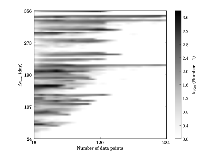
Figure 1: The number of data points and maximum time span for set A. Five test fields show a broad distribution in the number of data points. The maximum time span also reveals a broad distribution that does not depend on the number of data points.

We use light curves that have more than 15 good photometric data points in the NSVS database. A systematic search of the various kinds of variable sources has not been carried out with the NSVS data. But photometric quality control is well understood, and we can use the large amount of photometric data that allows us to recover new variable sources. We select five NSVS fields (065d, 087a, 088d, 135b, 135d) that have the largest number of objects in those fields. The basic information for those fields is given in Table 1 (Woźniak et al., 2004). We call these data set A. As Woźniak et al. (2004) suggested in their Table 3, we use only good photometric data points, which avoid any artifacts from observation and data processing, for each object. This photometric quality cut prevents any effects from spurious data points. When we limit samples that have more than 15 good photometric points, the number of objects from each field is about 45,000. The total number of objects is 227,212.

As shown in Figure 1, the number of data points and time-scale of light curves has a broad range. The number of data points in the light curves affects the uncertainties in the variability indices that will be explained in the following section. Furthermore, the number of data points is decided by a sampling pattern for each field as well as the selection of good photometric data. The extractable information is also subject to the time scale of the light curve. In the case of periodic variability, the Nyquist frequency is an important measurement (Koen, 2006). However, if we consider a general type of variability and irregular sampling, it is useful to examine the distribution of the maximum time span among data points. Only a tiny fraction of the light curves covers a time span of about 300 days with more than 100 data points, where a dominant fraction of the data has less than 60 data points.

Table 2: NSVS fields of the set B.

Name	Galactic $l$	Galactic $b$	Number of frames	Number of objects	Limiting photometric scatter
045a	99.0	-6.0	304	54455 (45551)	0.032
064a	66.0	9.0	308	54320 (46392)	0.028
089a	64.0	-13.0	289	54363 (46639)	0.025
112a	43.0	-9.0	228	54334 (43191)	0.031
135a	23.0	-2.0	112	54096 (40601)	0.037
157d	10.0	-10.0	61	54391 (4838)	0.031

The numbers in the parenthesis represent objects that have more than 15 good data points. We use a part of the data from field 157d.

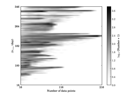
Figure 2: The number of data points and maximum time span for set B. Compared with set A, the light curves of set B have a smaller number of data points. Set B also covers a smaller time span than set A.

We also extract set B which has the same number of light curves from six different fields of the NSVS as set A. The differences between these two sets arise from the overall number of frames being larger in set B than in set A (Table 2). However, using only good photometric data points as we do with set A (see Woźniak et al., 2004, Table 3) makes the light curves of set B includes less data points than set A. Additionally, set B has fewer light curves with a large time-span and many data points as shown in Figure 2.

2.2 Variability indices

Figure 3: Light curves with minimum, median, and maximum parameter values. The left three columns present light curves with minimum, median, maximum values of $\sigma/\mu$, $Con$, and $\eta$. The right three columns are the same light curves but with $J$, $K$, and $AoVM$. Even among these examples, we recognise a light curve of a variable star with the smallest $\eta$, which is a known variable star BS Her (Nassau & Stephenson, 1961), because of its monotonic increasing magnitude. The light curve with the largest value of $Con$ shows a systematic variation that may be a variable star which corresponds to the infrared source IRAS 18402-1742 (Helou & Walker, 1988).

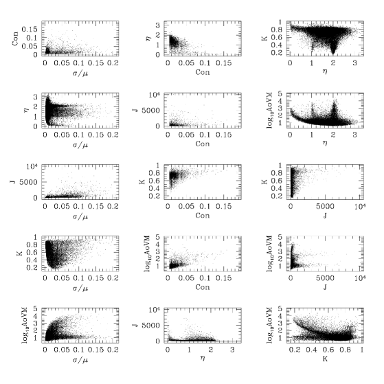
Figure 4: Distribution of variability indices for the set A. Each variability index describes a different feature of light curves in time domain. But we find the existence of the strong concentration of data in this six dimensions of the variability indices. It implies that the GMM can definitely find a dominant cluster of non-variable sources, while also separating outliers from the dominant cluster as separate minor clusters.

Below we define six variability indices ($\sigma/\mu$, $Con$, $\eta$, $J$, $K$, $AoVM$) that are obtained from light curves in the time domain. The simplest index of variability is the ratio of the standard deviation to the sample mean magnitude

$$\frac{\sigma}{\mu}~{}=~{}\frac{\sqrt{\sum_{n=1}^{N}(x_{n}~{}-~{}\mu)^{2}/(N~{}-~{}1)}}{\sum_{n=1}^{N}x_{n}/N},$$ (1)

where $n$ is an index over the relevant data points and $N$ is the total number of data points in each light curve. When this ratio is large, the light curve may have strong variability. We note that this ratio is not correspondent to a flux ratio because magnitude is a logarithmic unit.

However, $\sigma/\mu$ does not describe detailed features of variability. Therefore, we find three consecutive points that are at least 2 $\sigma$ fainter or brighter than the median magnitude in order to trace a continuous variation in the data points. The number of consecutive series is normalised by $(N-2)$, and is called Con . This measurement was used in Wozniak (2000).

The systematic structure of the light curves is also quantised by the ratio of the mean square successive difference to the sample variance $\eta$ (von Neumann, 1941):

$$\eta~{}=~{}\frac{\delta^{2}}{\sigma^{2}}~{}=~{}\frac{\sum_{n=1}^{N-1}(x_{n+1}~{}-~{}x_{n})^{2}/(N~{}-~{}1)}{\sigma^{2}}.$$ (2)

This von Neumann ratio was suggested to test the independence of random variables in successive observations particularly on a stationary Gaussian distribution. When there is a strong positive (negative) serial correlation between sequential data points, this ratio is small (large). In short, if serial correlation exists, the ratio is significantly high or small (Panik, 2005). The distribution of $\eta$ has been extensively investigated for a stationary Gaussian distribution (e.g. Bingham & Nelson, 1981), and its sample average and variance are well known (Williams, 1941). But the properties of $\eta$ are not simple for astronomical time-series data because they are irregularly sampled and do not follow a simple known distribution such as a stationary Gaussian distribution.

Three additional indices are adopted from concepts that have been developed in astronomy community. J and K are suggested by Stetson (1996). We use the following definition that uses only a single photometric band:

$$J~{}=~{}{\sum_{n=1}^{N-1}sign(\delta_{n}\delta_{n+1})\sqrt{|\delta_{n}\delta_{n+1}|}},$$ (3)

$$K~{}=~{}{\frac{{1/N}\sum_{n=1}^{N}|\delta_{n}|}{\sqrt{1/N\sum_{n=1}^{N}\delta_{n}^{2}}}},$$ (4)

where $\delta_{n}~{}=~{}\sqrt{N/(N-1)}(x_{n}-\mu)/e_{n}$ which has a photometric error for each data point $e_{n}$ and $sign(\delta_{n}\delta_{n+1})$ is the sign of $\delta_{n}\delta_{n+1}$. Finally, we measure the analysis of variance (ANOVA) statistic which is useful for discovering periodic signals (Schwarzenberg-Czerny, 1996). The maximum value of the ANOVA represented by AoVM is used to measure the strength of periodicity. Even though the corresponding period can be incorrect, the AoVM is still a valuable quantity that infers periodicity (Shin & Byun, 2007).

Figure 3 shows light curves with variability indices that have the minimum, median, and maximum values across all of the 227,212 light curves in set A. None of the light curves occur more than once in Figure 3. These examples prove that different variability indices catch different features of light curves. The light curve of the infrared source IRAS 18402-1742 (Helou & Walker, 1988) has the largest value of $Con$. We suspect that the variation of the light curve is real, and the star might be a long-period variable star. The light curve with the minimum value of $\eta$ corresponds to a known variable star BS Her (Nassau & Stephenson, 1961). As we expect, the positive serial correlation in magnitude has a small $\eta$ in this light curve.

The variability indices complement each other by picking up different features of the light curves. As shown in Figure 4, even though we notice some structure in the distributions for each two-dimensional projection of the original six-dimensional space, the indices do not have a strong correlation with each other. If a dominant fraction of light curves is simply from a Normal distribution, we would see only one simple structure in all plots. Since light curves of non-variable objects are not random samples from a Normal distribution, each plot shows more complicated structures which imply the existence of variable objects. Any structures will be defined as a separate cluster by the GMM. However, the strong concentration of data in each plot implies the existence of a dominant cluster of non-variable objects. Additionally, combining multiple indices helps us suppress the false detection of variable sources while not missing any possible features in the variability.

2.3 GMM

In the infinite GMM based on the DP, the distribution of mixture component members is described by a multivariate Gaussian distribution while the distribution of all objects is described by a mixture of Gaussian distributions defined by the stochastic DP. Each of the $M$ component distributions has the following form:

$$p_{m}(x)=\frac{1}{(2\pi)^{\gamma/2}|\Sigma_{m}|^{1/2}}\exp(-\frac{1}{2}({\bf x}-{\bf\mu_{m}})^{T}\Sigma_{m}^{-1}({\bf x}-{\bf\mu_{m}})),$$ (5)

where $m$ is an index over $M$, ${\bf x}=(\sigma/\mu,Con,\eta,J,K,AoVM)$ is a 6-dim vector of parameters, and $\gamma$ is the number of parameters (in our case $\gamma=6$). Furthermore, ${\bf\mu_{m}}$ is a $6$-dim vector of mean values (i.e., mixture centres), and $\Sigma_{m}$ is the covariance matrix of the Gaussian distribution associated with the $m$th mixture component. The problem is how to find a weighting for each mixture component $w_{m}$ and its respective $\mu_{m}$ and $\Sigma_{m}$ such that the final distribution of all objects is given by:

$$p({\bf x})=\sum_{m=1}^{M}p_{m}({\bf x})w_{m}.$$ (6)

The DP is used to estimate $w_{m}$, $\mu_{m}$, and $\Sigma_{m}$ and is explained in Appendix A.

When loading a given data set, one also specifies initial values for hyper-parameters used in the clustering algorithm. These hyper-parameters include the number of iterations to be taken by the algorithm to ensure convergence to a stable model, number of initial mixture components $M$ to which data is assigned, and concentration $\alpha$ which can be thought of as the inverse variance of the DP. In all of the models presented in this paper, the number of iterations is 100 even though convergence can be seen in as little as 10 iterations, $M=60$ initially, and $\alpha=1$. Convergence is defined by $M$ reaching some consistent value despite the algorithm continuing to iterate. To ensure that the clustering algorithm identifies all relevant features (i.e., number of mixture components), it is possible to initialise the algorithm with $M=N$, (i.e. the number of data points) which is the highest possible complexity. Since we are mainly concerned with identifying one central cluster (i.e., non-variable objects), this computationally expensive procedure is unwarranted. With the data set and hyper-parameters loaded, the algorithm first creates an empty Gaussian distribution $G_{0}$ of mixture components $M$ with a conjugate Gaussian-Wishart prior such that the mean vector is drawn from a Gaussian distribution and precision matrix (i.e., the inverse covariance matrix $\Sigma_{m}^{-1}$) is drawn from a Wishart distribution. Second, the algorithm randomly initialises the mixture component assignments $z=\lceil R_{N}M\rceil$, where $R_{N}$ is a $N$-dim vector with entries that are uniformly distributed. By using $\alpha$, $G_{0}$, and $z$, data points ${\bf x}$ are added to the mixture components. As the algorithm iterates to convergence, this initial assignment matters little because conditional probabilities are computed for each data point with respect to each of the $M$ active mixture components. Lastly, a collapsed Gibbs sampler runs for the specified number of iterations while also iterating over $N$. We implement this algorithm by using MATLAB.

3 The largest cluster as non-variable objects

Since the largest cluster must represent non-variable light curves, and our GMM with the DP is a data-driven unsupervised machine learning algorithm, the properties of the largest Gaussian mixture must be dependent on the input data. Therefore, we examine the dependence of results on the size and properties of the input data.

Figure 5: The change in cluster properties for set A as a function of the number of iterations. (a) The total number of identified clusters converges to 29 after 10 iterations. (b) The number of data in the largest cluster reaches 82%, but converges to 76% after 100 iterations. (c - h) The center of the largest cluster does not show a significant change after the 10th iteration. It means that the small changes in the number of clusters after the first 10 iterations does not affect the Gaussian model of the largest cluster.

3.1 Results of set A

The GMM of set A is composed of 29 mixture components where one cluster dominates the data. As shown in Figure 5, the number of mixture components quickly converges to about 29 after 10 iterations. Moreover, the centre of the dominant cluster remains stationary. The largest cluster is populated by 76.2% of the input data, and describes non-variable objects. The second and third largest clusters include only 7.7% and 5.6% of the data, respectively.

The centre of the dominant cluster is ($\sigma/\mu$ , Con , $\eta$ , J , K , AoVM ) = ($7.45\times 10^{-3}$, $3.90\times 10^{-9}$, $1.70$, $8.29$, $7.52\times 10^{-1}$, $8.16$), which also becomes stationary when the number of clusters converges after the 10 iterations. The covariance of the multivariate Gaussian model for the largest group is used for statistical inference to select candidates that may be variable sources and will be explained in §4. Measuring the ratio between the covariance of each variability index for the largest cluster and that for the whole data of set A, we find that the ratio of $\eta$ is 0.71 which is highest among the six variability indices. Meanwhile, the ratio of Con is lowest and close to zero, suggesting that this variability index has less powerful than others in separating out non-variable objects.

Figure 6: The change in cluster properties for randomly selected 10%, 30%, and 50% samples of set A. In each plot, the cross symbol corresponds to the converged values given in Figure 5. (a) The total number of identified clusters is smaller than that of the original dataset. The subsets are represented as dotted, dashed, and solid lines for 10%, 30%, and 50%, respectively. (b) The largest cluster in the samples has a higher percentage of the data than the largest cluster in the original dataset. (c - h) For all six variability indices, the result for the 50% subset is most close to what we find for the entire data.

3.2 Dependence on the size of data

Table 3: Changes of the largest group in the 10%, 30%, and 50% samples.

Fraction of data	Included non-variables	Recovered non-variables	Included variables	Missed non-variables
10%	17368	17348 (99.9)	1082 (6.2)	20 (0.1)
30%	52043	51860 (99.6)	2856 (5.5)	183 (0.4)
50%	86818	86070 (99.1)	2696 (3.1)	748 (0.9)

The numbers in parenthesises show the fraction in percentage with respect to the total number of non-variable members (i.e. the second column) that were included in the largest group associated with the original dataset and that are also included in the largest cluster associated with the subsamples.

Figure 7: Distribution of the Mahalanobis distances from the largest group with the original data for 10%, 30%, and 50% subsamples. In each plot, the distribution for all data points (i.e. the original data) is represented by dotted lines, while solid lines are the distributions of objects which are included in the largest group associated with both the sub-samples and the original data. Objects newly included in the largest group associated with the sub-samples (dashed line) and excluded from that (shaded bar) are mainly from the edge of the original largest group. The distribution represents $dN/dlog_{10}D_{M}$ instead of $dN/dD_{M}$.

The dependence of the largest cluster on the size of the input data is tested using samples of set A. We randomly select 10%, 30%, and 50% of the light curves from set A. We compute a GMM for these sub-samples using the same setup that was used for the main test. Following the basic assumption that the largest cluster represents non-variable objects, we identify the largest cluster in the three subsets. The GMM for the 50% sample should be closer to the GMM for all of set A than the GMMs for 10% and 30% samples.

The six variability indices show dependencies on the size of the input data. In Figure 6, the GMM recovers more clusters as the size of dataset increases. Because a larger dataset can include more features of data, the GMM finds more separable clusters. This result is consistent with our expectation for an infinite GMM based on the DP which identifies previously unseen structure as the data set with observable features increases in size. Although each variability index responds differently to the size of data, all indices converge more quickly with less data. But the result for the 50% subset shows the better convergence of the indices to the original values than other subsets.

However, more iterations do not make it possible to recover more clusters. When we use set A, we find 29 clusters with 100 iterations, and the number of clusters quickly converges to 29 after 10 iterations. But a smaller data produces less clusters more quickly. Unsupervised learning techniques naturally handle variation in the size of dataset which correspond to variation in the amount of available information. Therefore, the maximum number of recovered clusters is not dependent on how many times the clustering procedure iterates.

We test the stability of the largest group derived with the original data by checking the membership of the largest groups with 10%, 30%, and 50% samples. For example, 10% subsamples have 17368 data points which were included in the largest group as shown in Table 3. Among those data points, 99.9% of them are recovered in the largest group with 10% subsamples, while 1082 objects are newly included in the largest group. However, 20 objects are now enclosed in minor groups with 10% subsamples. In both 30% and 50% subsamples, the members of the original largest group are well recovered with higher than 99% rate. The clustering result is mainly affected by new objects which were not included in the largest group associated with the original data, but are included into the largest group associated with the sub-samples. These data points are mainly from the edge of the largest group in the original data as shown in Figure 7. The definition of the Mahalanobis distance $D_{M}$ is

$$D_{M}=\sqrt{(\bf{x}-\bf{\mu}_{0})^{T}\Sigma_{0}^{-1}(\bf{x}-\bf{\mu}_{0})},$$ (7)

where the centre $\bf{\mu}_{0}$ and covariance matrix $\Sigma_{0}$ of the largest cluster with the original data are used with the position of an individual object $\bf{x}$ in six-dimensional space. Simply, $D_{M}$ corresponds to the exponent of the multivariate Gaussian distribution (see Equation 5). Therefore, a high value of $D_{M}$ represents a distant object from the centre of the largest group. Figure 7 shows that contamination related to the largest group is dominated by objects around the edge of the original largest group.

3.3 Dependence on the noise in data

Figure 8: Example light curves with increased dispersions. From top to bottom, each panel shows the raw light curve and light curves with 10%, 30%, and 50% increased dispersions, respectively. The dispersion of the raw light curve is increased by adding random values that sampled from a Normal distribution to the existing raw data points.

Figure 9: The change in cluster properties for set A with 10%, 30%, and 50% increased dispersions. In each plot, the cross symbol corresponds to the converged values given in Figure 5, and dotted, dashed, and solid lines represent 10%, 30%, and 50% increased dispersions, respectively. (a) The total number of identified clusters is higher than that of the original dataset. (b) The fraction of data in the largest cluster decreases substantially compared with the largest cluster associated with the original data. (c - h) Six variability indices have different sensitivities to the change in magnitude dispersion, implying that variability indexes are important to clustering.

Table 4: Changes of the largest group in the samples with 10%, 30%, and 50% increased dispersions.

Increased dispersions	Recovered non-variables	New non-variables	Excluded non-variables
10%	146170 (84.4)	1808 (1.0)	27017 (15.6)
30%	141332 (81.6)	3724 (2.2)	31855 (18.4)
50%	143689 (83.0)	6998 (4.0)	29498 (17.0)

The numbers in parenthesises show the fraction in percentage with respect to the total number of members that were included in the largest group associated with the original data.

In order to test the effects of noise on the clustering results, we modify the original data set A by adding extra dispersions to the raw light curves. If the magnitude distribution in the raw light curves is simply described by the Normal distribution $N(\mu,\sigma^{2})$ with mean $\mu$ and dispersion $\sigma^{2}$, we can increase the dispersion of the light curve by adding the random number from the Normal distribution $N(0,\sigma_{add}^{2})$ to the raw light curve, because the sum of two Normal distribution variables also follow Normal distribution:

$$U=X+Y\sim N(\mu_{X}+\mu_{Y},\sigma_{X}^{2}+\sigma_{Y}^{2}),$$ (8)

where $X\sim N(\mu_{X},\sigma_{X}^{2})$ and $Y\sim N(\mu_{Y},\sigma_{Y}^{2})$. Here, we do not change the time sequence of the raw light curve, and use the dispersion of the raw light curve to generate the added term with the three cases of $\sigma_{add}^{2}=0.1\sigma^{2},0.3\sigma^{2}$, and $0.5\sigma^{2}$. These values correspond to 10%, 30%, and 50% increases in dispersions, respectively. Figure 8 shows one example light curve which is a member of the largest group associated with the original data.

We warn that our approach to degrade the data can be quite different from realistic cases. First, there is no guaranty of assuming a Normal distribution for the raw light curves. Second, even when raw light curves follow a Normal distribution, the rule given in Equation 8 is not well implemented when light curves have a small number of data points. Third, if the raw light curve has intrinsic variability which might result in a large dispersion, using the dispersion from the raw light curve in Equation 8 can cause systematically biased effects on the light curves of truly variable objects. Because of these reasons, the increase in dispersion can deviate from the expected change in Equation 8 as shown in Figure 8. Our simulation also fails to reproduce red noise if the data have. Even though this test might not be realistic, unsupervised learning intrinsically lacks a way to study noise effects without providing completely artificial data.

Figure 10: Distribution of the Mahalanobis distances from the original largest group for the samples with 10%, 30%, and 50% increased dispersions. The distribution for the original data is described by dotted lines. For the members of the original largest group, parts of them are still included in the largest group with the noise data (solid line; the second column in Table 4) even after they were altered by added dispersions. But as the dispersion increases, more objects (shaded histogram; the third column in Table 4) are newly included in the largest group with the noise data, while some members of the largest group with the original data (dashed line; the fourth column in Table 4) are now excluded from the new largest group.

Figure 9 summarises the effects of noise on clustering and the largest group. The increase in noise enhances dispersions among clusters that were found with the original data, and results in the recovery of more clusters because the largest group is populated by fewer objects. Importantly, variability indices associated with the centre of the largest group responds to the effects of noise in different ways. Therefore, the change of the cluster centre for the largest group is not a simple function of the dispersion change although the data with the low noise generally converges to the results for the original data.

Figure 11: Distribution of the Mahalanobis distances from the new largest group in the samples with the increased dispersions. The solid line shows the distribution of all objects with respect to the new largest group. The dashed line and shaded histogram represent the same objects as explained in Figure 10. The top two largest clusters are shown by dotted lines for each case.

We also trace which objects are included in the newly found largest cluster. The added dispersion naturally boosts mixing between the original largest group and other minor groups. As presented in Table 4, about 16% - 18% of objects that were included in the largest group associated with the original data are found in minor groups with the increased dispersions. Meanwhile, the addition of new objects to the largest group is a small percentage. Figures 10 and 11 show that the increased dispersions induce the objects around the edge of the original largest cluster to move from the largest cluster in the new clustering. Figure 11 demonstrates that this effect mainly results in grouping objects into the second largest cluster in the new data.

3.4 Dependence on the source of data: results of set B

We test the dependence of the GMM on the properties of a particular dataset by applying our method to set B. As described in §2.1, set B has different properties of data. The largest cluster of set B is populated by 83.1% of data, while we find that the largest cluster of set A is populated by 76.2% of the data (see Figure 12). The number of recovered clusters is 26 which is smaller than that of set A. Even though fewer clusters are identified in set B, the largest cluster in set B describes more of the data.

Figure 12: The change in cluster properties for set B. The plotted fields are the same as those in Figure 5. We find some difference in the largest cluster between sets A and B as we expect in data-driven machine learning. In particular, $J$ shows the most significant difference.

Figure 12 shows how each variability index changes based on the input data. In this test, $J$ is a signature of a large change that depends on the properties of the data. We note that $K$ or $AoVM$ is a variability index that shows the largest change for the noisy data (see Figure 9). The centre of the largest cluster in set B is ($\sigma/\mu$ , Con , $\eta$ , J , K , AoVM ) = ($6.84\times 10^{-3}$, $3.45\times 10^{-9}$, 1.68, $6.41\times 10^{-2}$, $7.52\times 10^{-1}$, 7.75). This result implies that our method has to be applied to a single dataset that shares common properties. This requirement is often necessary for data-oriented machine learning methods. Compared to the test associated with increasing the dispersion of light curves, the experiment with set B is more realistic in proving the data-dependence of unsupervised machine learning algorithms.

4 Separation of variable objects

After we identify the largest cluster as the aggregation of non-variable objects, the next question is how to separate out candidates of variable objects. Naively, we can accept the clustering results of the GMM as a guide line for the separation. But simply depending on clustering results is not satisfactory for two reasons. First, any systematic spurious patterns can be clustered as the second or third largest cluster, as seen in Figure 11. Second, some clusters can be close to the largest cluster in six-dimensional space, implying that the separation of other clusters from the largest cluster might not be meaningful. Therefore, if the clustering result is used to define candidates of variable objects, then various classical methods for multivariate analysis can be applied (Krzanowski, 1988) in addition to the cluster membership from the GMM with the DP. We suggest two simple ways to use the results from our GMM method with the clustering membership.

4.1 Inference from Mahalanobis distances

The first approach uses the Mahalanobis distance to gauge how far an object is from the largest cluster. For our application, the Mahalanobis distance is more useful than a multidimensional norm because it includes the effects from the dispersion of the data (Bishop, 2006).

Figure 13: Mahalanobis distance of all objects in set A. The distribution of all objects (thick solid line) has a peak around $D_{M}\sim 2$ which corresponds to the distribution of only the largest cluster (thin solid line). The second and third largest clusters (dotted lines) are distributed closely to the largest cluster, even though they are identified separately by the GMM with the DP.

The distribution of $D_{M}$ shown in Figure 13 indicates that a cut based on $D_{M}$ can be used to identify variable objects. This distribution has a concentration of objects around $D_{M}\sim 2$. The position of this peak matches the mode value of the Beta distribution which is expected for the distribution of $D_{M}$ (Ververidis & Kotropoulos, 2008). This distance also represents the typical distance of objects that are included in the cluster of non-variable objects (i.e. the largest cluster). Furthermore, this distribution confirms that the second and third largest clusters may not represent real variable objects because the members of the clusters are close to the largest cluster.

Even though $D_{M}$ is inexpensive to compute, it does not give direct statistical inference nor provide a statistical confidence limit on our belief that an object is variable. $D_{M}$ is simply an exponent of the multivariate Gaussian distribution (see Equation 7). One has to find an empirical cut for $D_{M}$ that separates variable and non-variable objects.

4.2 Confidence bounds

The way to extract a direct statistical inference is to derive confidence bounds for non-variable objects with $D_{M}$. With the identified centre $\bf{\mu_{0}}$ and covariance matrix $\Sigma_{0}$ of the largest cluster, we define a confidence bound of 100$b$% (0 $<b<$ 1) which encompasses 100$b$% of non-variable objects (see Chen, Morris, & Martin, 2006, for an example). The confidence bound is described as a likelihood threshold $h$ that is associated with the probability $b$:

$$\int_{\bf{x}:p(\bf{x})>h}p(\bf{x}|\bf{\mu_{0}},\Sigma_{0})d\bf{x}=b,$$ (9)

where $p(\bf{x})$ is a multivariate Gaussian distribution defined by $\bf{\mu_{0}}$ and $\Sigma_{0}$. From this integration, we can estimate a confidence limit that corresponds to a specific $D_{M}$ for $h$. But despite its statistical robustness, this integration is practically difficult and expensive to compute because it cannot be calculated analytically.

We use a Monte Carlo method to find the confidence limit in Equation 9. An approximate cut is simply the value of $D_{M}$ that includes 100$b$ % of the data in the largest cluster, when sorting $D_{M}$ in an ascending order, i.e. a descending order of $p$. However, a more precise estimate is made possible by generating multiple samples of the data that populate the largest cluster and finding a limit for $D_{M}$ in each sample (Chen, Morris, & Martin, 2006). In Figure 13, we can guess that $D_{M}=4.67$ for set A where an approximate cut of 99% is assumed. But we find $D_{M}=4.68$, when using the Monte Carlo method by sampling 50 times with 2000 samples for each sampling. Because the largest group includes a large number of data points, the simple approximation is close to the estimate given by the Monte Carlo method. When we choose a 90% cut in $D_{M}$ to define variable source candidates, the total number of candidates is 50,394 for set A and corresponds to about 22% of the light curves. But we find that about 9% and 29% of objects in the second and third largest group are within the 99% cut of the largest group (i.e. $D_{M}=4.68$).

4.3 Examples of light curves for each cluster

Our method provides two pieces of information to help people select variable source candidates. First, objects are chosen as candidates when they are not included in the largest cluster. This idea corresponds to a classical method of outlier detection which uses clustering. Second, we use the cut $D_{M}$ in addition to the result of clustering. As shown in Figure 13, the second and third largest clusters are overlapped with the largest cluster in the six-dimensional space. This second approach is relevant to the distance-based outlier detection (Cateni, Colla, & Vannucci, 2008). The most useful approach is to employ both the clustering results and the statistical cut in $D_{M}$. If we conclude that the second and third largest clusters are explained by a systematic bias in the data, then we can exclude the second and third largest clusters when selecting variable source candidates. Furthermore, $D_{M}$ can be used to assign a priority to the candidates.

Figure 14: An example of light curves for clusters 1, 2, 3, and 4. The second light curve for cluster 3 with $D_{M}=93.5$ is matched to a known variable star SV* BV 1711 (Strohmeier & Knigge, 1975), while the second light curve for cluster 4 is IRAS 19225-0740 (Helou & Walker, 1988).

Figure 15: Example light curves for clusters 5 - 12. None of these examples are known variable stars. Cluster 7 is the largest cluster which represents non-variable objects. Both light curves of cluster 6 show a recognisable change in brightness even with poor sampling of the light curves. Cluster 10 is the second largest cluster that has some objects within the 99% cut of $D_{M}\sim 4.7$

Figure 16: Example light curves for clusters 13 - 20. No known variable sources were found for these example objects within the 6$\aas@@fstack{\prime\prime}$0 search radius using the SIMBAD. But both examples of cluster 17 show long-period variability. Additionally, the examples of cluster 16 might be eclipsing binaries. Cluster 13 is the third largest cluster, and includes about 6% data of set A.

Figure 17: Example light curves for clusters 21 - 29. Except for clusters 28 and 29 which have only one member, two examples are presented for each cluster. The first example of cluster 21 spatially corresponds to IRAS 20302+1938 (Helou & Walker, 1988). The second example with $D_{M}=7.22\times 10^{7}$ is the infrared carbon star IRAS 18364+1757 (Helou & Walker, 1988; Guglielmo et al., 1993). While the first example of cluster 22 is the known variable star V* V2328 Cyg (Dahlmark, 2001), the second example is not a known variable object even though its light curve shows a clear sign of variability. For cluster 26, the first example is a Mira-type variable star V* Z Del (Templeton, Mattei, & Willson, 2005).

Figure 14 presents an example of light curves for clusters 1, 2, 3, and 4 in set A. Here, we randomly select two light curves for each cluster. Cluster 1 is the fourth largest cluster in the GMM for set A. In order to check for known variable sources in our samples, we spatially match our samples to the SIMBAD database (Genova, 2007) using a 6$\aas@@fstack{\prime\prime}$0 search radius. For cluster 3, the second object is the known variable star SV* BV 1711 (Strohmeier & Knigge, 1975). The second object for cluster 4 is the known infrared source IRAS 19225-0740 (Helou & Walker, 1988) which may be a long-period late-type variable star.

For the rest of the identified clusters in set A, we also randomly extract two example objects. These light curves are presented in Figures 15, 16, and 17. Only a small number of objects among the examples are known variable stars or infrared sources that might be long-period variable stars. The clusters 10 and 13, corresponding to the second and third largest cluster respectively, show similarities in their light curves to those of the largest cluster (i.e. the cluster 7). Because of poor sampling for short-period variable sources in the NSVS, it is not likely for us to recognise periodic short variability in the example light curves.

5 Discussion and Conclusion

We presented a new framework for discovering variable objects in massive time-series data with variability indices which have been commonly used in astronomy. Our method is fully non-parametric and depends on only one assumption: the largest cluster represents a group of non-variable objects. The infinite GMM with the DP derives a mixture of multivariate Gaussian distributions from the given data consisting of six variability indices. With these results, we use the clustering results and Mahalanobis distances from the largest cluster to select variable object candidates.

Our application of the infinite GMM with the DP for clustering may be useful for measuring how efficiently we recover variable objects depending on various factors. Before designing the observation strategy to acquire time-series data, simulated data can be applied to our method. This test will help people understand what kind of variability is missed in the data given by a specific observation strategy and environment.

Pre-processing the time-series data, i.e. feature extraction and selection, can affect the results of the infinite GMM with the DP. This effect has been seen in other unsupervised clustering algorithms, too (Jain et al., 1999). In this paper, we only use six variability indices which are mainly developed for astronomical time-series data. Unlike time-series data in other fields, astronomical time-series data are irregularly sampled and less homogeneous. This difference makes pre-processing of our data with a common method such as principal component analysis difficult. Moreover, finding the best features for unsupervised clustering is a trial-and-error problem (Jain et al., 1999). In the framework of the GMM with the DP, the importance of each variability index is reflected in each Gaussian component’s covariance matrix which also describes the compactness of the found clusters. Therefore, the combination of the best features will be dependent of the input data, while making this study be a trial-and-error problem (Dy & Brodley, 2004). In the next paper of this series, we will investigate the usefulness of a variety of variability indices for the infinite GMM with the DP.

Finally, simply selecting variable star candidates with the unsupervised learning method is not useful without analysing what kind of objects are selected as candidates. Our approach also uses unlabelled data which we do not know any physical properties about. It is necessary to figure out properties of the selected candidates in the further analysis of variable time-series data.

We showed that our method is a fully data-driven approach such that the method itself finds its best separation of variable objects for the given data. This property makes our idea easily applicable to future projects such as Pan-STARRS (Kaiser, 2004), GAIA (Eyer & Cuypers, 2000), and LSST (Walker, 2003) as well as archives of the past surveys such as MACHO (Cook et al., 1995). In another paper, we will provide a full list of variable object candidates from the NSVS for each observation field.

Appendix A Bayesian Non-parametric Clustering

Bayesian nonparametric clustering algorithms based on the Dirichlet Process are a powerful way to model and manipulate data in statistics, machine learning, and signal processing. In this type of analysis, Bayesian refers to the manner in which one estimates the likelihood of an event given information in the data set about all known events and nonparametric refers to the manner in which a set of events can be modelled such that the structure of the model is determined only by the data set. Since Bayesian nonparametric techniques are not based on prior assumptions about the structure, number of mixture components, or location of components in a data set, one employs the Dirichlet Process to assign a prior probability (i.e., the unconditional probability of an event before relevant information is considered) to a data point $x_{n}$ such that the stochastic generative process draws from a distribution of distributions (in our case, a mixture of multivariate Gaussian distributions) (Ferguson, 1973; Antoniak, 1974; Jordan, 2005).

The Dirichlet Process mixtures are also referred to as infinite mixtures because although data may exhibit a finite number of components, new data can exhibit previously unseen structure (Neal, 2000; Blei & Jordan, 2004). Therefore, these models adjust their complexity according to the complexity of the data and mitigate under-fitting the data (Teh, 2007). In this unsupervised algorithm, no data points were discarded as background.

To understand the Dirichlet Process and our Bayesian nonparametric clustering algorithm, we explain the following ideas from probability theory. Let $\eta$ be a probability space, $G_{0}$ be a distribution over $\eta$, and $\alpha$ be a positive real number (in our case, $\alpha=1$). Therefore, a random distribution $G$ over $\eta$ is said to be Dirichlet Process distributed:

$$G\sim\textrm{DP}(\alpha,G_{0}),$$ (10)

if and only if for all natural numbers $j$ and any finite partition $(A_{1},\ldots,A_{j})$ of $\eta$, the random vector $(G(A_{1}),\ldots,G(A_{j}))$ is distributed as a finite-dimensional Dirichlet distribution:

$$(G(A_{1}),\ldots,G(A_{j}))\sim\textrm{Dir}(\alpha G_{0}(A_{1}),\ldots,\alpha G_{0}(A_{j})),$$ (11)

where $G_{0}$ is the base distribution of $G$ (i.e., mean of the Dirichlet Process) and $\alpha$ is the concentration parameter (i.e., inverse variance of the Dirichlet Process) (Blei & Jordan, 2004; Jordan, 2005; Teh, 2007).

Bayesian nonparametric clustering based on the Dirichlet process can be applied to $N$-dim data with multiple parameter fields $(x_{1},\ldots,x_{N})$ provided that the data is regarded as being part of an indefinite exchangeable sequence. One models the distribution from which $x$ is drawn as a mixture of distributions of the form $F(\eta)$, with the mixing distribution over $\eta$ being $G$, which has the Dirichlet Process as a nonparametric prior probability. Therefore, the Dirichlet Process mixture model is represented as (Ferguson, 1973; Antoniak, 1974; Neal, 2000; Blei & Jordan, 2004; Teh, 2007):

$$G \sim \textrm{DP}(\alpha,G_{0}),$$ (12)

$$\eta_{m}|G \sim G,$$ (13)

$$x_{n}|\eta_{m} \sim F(\eta_{m}).$$ (14)

Since the parameters $\eta$ are drawn from $G$, the data $x$ clusters according to the values of $\eta$. For the cluster model presented in this work, $x$ is drawn from $F$, which is assumed to be a mixture of multivariate Gaussian distributions. Therefore, $\eta_{m}\rightarrow(\mu_{m},\Sigma_{m})$, where $\mu_{m}$ is the mean and $\Sigma_{m}$ is the covariance matrix for the $m^{th}$ mixture component.

In Dirichlet Process mixture modelling, the posterior distribution on the partitions (i.e., the conditional probability of the mixture components) is intractable to compute. However, Markov chain Monte Carlo methods allow one to approximate posteriors by constructing a Markov chain that is easy to implement for models based on conjugate prior distributions such as the Gaussian distributions used in this paper (Neal, 2000; Blei & Jordan, 2004). The most widely used inference method is the Gibbs sampler because of its simplicity and good predictive performance. In the Gibbs sampler, the Markov chain is obtained by iteratively sampling each variable that is conditioned on the data and other previously sampled variables. If one integrates out all random variables except $q_{m}$ (i.e., mixture component that the $n^{th}$ data point $x_{n}$ is associated with), then one arrives at the collapsed Gibbs sampler, which iteratively draws each $q_{m}$ from the following expression (Blei & Jordan, 2004):

$$p(q_{m}=1|x,q_{-m},\lambda,\alpha)\propto p(x_{n}|x_{-i},q_{-m},q_{m}=1,\lambda)p(q_{m}=1|q_{-m},\alpha),$$ (15)

where $q_{-m}$ denotes all of the previously sampled cluster variables except for the $m^{th}$ variable and $\lambda$ is a hyper-parameter that is used to define the base distribution $G_{0}$. The first term on the right-hand side of Equation 15 is a combination of normalising constants that comes from considering Dirichlet Process mixtures for which data is drawn from an exponential family (e.g., Gaussian distribution). The second term on the right-hand side is:

$$p(q_{m}=1|q_{-m},\alpha)=\left\{\begin{array}[]{ll}\frac{n_{m}}{N-1+\alpha}&~{}~{}\textrm{seen component}\\ \frac{\alpha}{N-1+\alpha}&~{}~{}\textrm{unseen component}\end{array}\right.,$$ (16)

where $n_{m}$ is the number of members in $q_{m}=1$. Equation 16 comes from the partition structure of the Dirichlet Process and is the heart of the algorithm’s clustering effect such that the more frequently an event (i.e., a mixture component) is sampled in the past - the more likely the event is to be sampled in the future (Blei & Jordan, 2004). Once the Markov chain has run for a sufficiently long duration, samples of $q$ will be samples from $p(q|x,\alpha,\lambda)$ and one can construct an empirical distribution to approximate the posterior.

The collapsed Gibbs sampler runs for a specified number of iterations and also iterates over the number of data items $N$. The method proceeds with the following steps (Teh, 2007):

1. Remove data item $x_{n}$ from component $q_{m}$, where $m$ specifies the cluster to which data item $n$ belongs

2. Delete the active component $q_{m}$ if it has become empty

3. Compute conditional probabilities $(p_{1},\ldots,p_{M})$ with respect to data item $x_{n}$ belonging to each of the $M$ active components $(q_{1},\ldots,q_{M})$

4. Choose new component identity $m$ by sampling from the conditional probabilities

5. If $m=M+1$, then create a new active component

6. Add data item $x_{n}$ into component $q_{m}$

References

- Antoniak (1974) Antoniak C., 1974, The Annals of Statistics, 2, 1152
- Akerlof et al. (1994) Akerlof C., et al., 1994, ApJ, 436, 787
- Alcock et al. (1995) Alcock C., et al., 1995, AJ, 109, 1653
- Alcock et al. (1996) Alcock C., et al., 1996, AJ, 111, 1146
- Alcock et al. (1997) Alcock C., et al., 1997, AJ, 114, 326
- Bamford et al. (2008) Bamford S. P., Rojas A. L., Nichol R. C., Miller C. J., Wasserman L., Genovese C. R., Freeman P. E., 2008, MNRAS, 391, 607
- Bishop (2006) Bishop C. M., 2006, Pattern Recognition and Machine Learning, Springer
- Blei & Jordan (2004) Blei D. M., Jordan M. I., 2004, Variational methods for the Dirichlet process, Proceedings of the International Conference on Machine Learning
- Bingham & Nelson (1981) Bingham C., Nelson L. 1981, Technometrics, 23, 285
- Belokurov, Evans, & Du (2003) Belokurov V., Evans N. W., Du Y. L., 2003, MNRAS, 341, 1373
- Belokurov, Evans, & Le Du (2004) Belokurov V., Evans N. W., Le Du Y., 2004, MNRAS, 352, 233
- Bono & Cignoni (2005) Bono G., Cignoni M., 2005, ESASP, 576, 659
- Cateni, Colla, & Vannucci (2008) Cateni S., Colla V., Vannucci M. 2008, Advances in Robotics, Automation and Control, IN-TECH
- Carbonell, Oliver, & Ballester (1992) Carbonell M., Oliver R., Ballester J. L., 1992, A&A, 264, 350
- Chattopadhyay et al. (2007) Chattopadhyay T., Misra R., Chattopadhyay A. K., Naskar M., 2007, ApJ, 667, 1017
- Chen, Morris, & Martin (2006) Chen T., Morris J., Martin E., 2006, Journal of the Royal Statistical Society: Series C (Applied Statistics), 55, 699
- Cook et al. (1995) Cook K. H., et al., 1995, ASPC, 83, 221
- Dahlmark (2001) Dahlmark L., 2001, IBVS, 5181, 1
- Debosscher et al. (2007) Debosscher J., Sarro L. M., Aerts C., Cuypers J., Vandenbussche B., Garrido R., Solano E., 2007, A&A, 475, 1159
- Dy & Brodley (2004) Dy J. G., Brodley C. E., 2004, The Journal of Machine Learning Research, 5, 845
- Eyer & Cuypers (2000) Eyer L., Cuypers J., 2000, ASPC, 203, 71
- Eyer & Blake (2002) Eyer L., Blake C., 2002, ASPC, 259, 160
- Eyer (2005) Eyer L., 2005, ESASP, 576, 513
- Eyer (2006) Eyer L., 2006, ASPC, 349, 15
- Eyer & Mowlavi (2008) Eyer L., Mowlavi N., 2008, JPhCS, 118, 012010
- Ferguson (1973) Ferguson T., 1973, The Annals of Statistics, 1, 209
- Genova (2007) Genova F., 2007, ASPC, 376, 145
- Guglielmo et al. (1993) Guglielmo F., Epchtein N., Le Bertre T., Fouque P., Hron J., Kerschbaum F., Lepine J. R. D., 1993, A&AS, 99, 31
- Helou & Walker (1988) Helou, G., & Walker, D. W. 1988, Infrared astronomical satellite (IRAS) catalogs and atlases. Volume 7, p.1-265
- Jain et al. (1999) Jain A. K., Murty M. N., Flynn P. J., 1999, ACM Computing Surveys, 31, 264
- Jordan (2005) Jordan M., 2005, Dirichlet processes, Chinese restaurant processes, and all that, Proc. 19th Annual Conf. on Neural Information Processing Systems (NIPS 2005), Neural Information Processing Systems Foundation.
- Kaiser (2004) Kaiser N., 2004, SPIE, 5489, 11
- Kelly & McKay (2004) Kelly B. C., McKay T. A., 2004, AJ, 127, 625
- Koen (2006) Koen C., 2006, MNRAS, 371, 1390
- Krzanowski (1988) Krzanowski W. J., 1988, Principles of Multivariate Analysis: A user’s perspective, Volume 3 of Oxford Statistical Science Series
- Mahabal et al. (2008) Mahabal A., et al., 2008, AN, 329, 288
- M’́uller & Quintana (2003) M’́uller P., Quintana F. A., 2003, Statistical Science, 19, 95
- Nassau & Stephenson (1961) Nassau J. J., Stephenson C. B., 1961, ApJ, 133, 920
- Neal (2000) Neal R. M., 2000, Journal of Computational and Graphical Statistics, 9, 249
- Paczyński (2000) Paczyński B., 2000, PASP, 112, 1281
- Paczyński (2001) Paczyński B., 2001, misk.conf, 481
- Panik (2005) Panik M. J., 2005, Advanced statistics from an elementary point of view, Academic Press
- Reimann (1994) Reimann J. D., 1994, PhDT,
- Schwarzenberg-Czerny (1996) Schwarzenberg-Czerny A., 1996, ApJ, 460, L107
- Schwarzenberg-Czerny (1998) Schwarzenberg-Czerny A., 1998, BaltA, 7, 43
- Shin & Byun (2004) Shin M.-S., Byun Y.-I., 2004, JKAS, 37, 79
- Shin & Byun (2007) Shin M.-S., Byun Y.-I., 2007, ASPC, 362, 255
- Stetson (1996) Stetson P. B., 1996, PASP, 108, 851
- Strohmeier & Knigge (1975) Strohmeier W., Knigge R., 1975, BamVe, 10, 116
- Sumi et al. (2005) Sumi T., et al., 2005, MNRAS, 356, 331
- Teh (2007) Teh Y. W., 2007, Dirichlet processes: tutorial and practical course, Machine Learning Summer School
- Templeton, Mattei, & Willson (2005) Templeton M. R., Mattei J. A., Willson L. A., 2005, AJ, 130, 776
- Ververidis & Kotropoulos (2008) Ververidis, D., & Kotropoulos, C. 2008, IEEE Transactions on Signal Processing, 56, 2797
- von Neumann (1941) von Neumann J., 1941, The Annals of Mathematical Statistics, 12, 367
- Walker et al. (1999) Walker S. G., Damien P., Laud P. W., Smith A. F. M., 1999, Journal of Royal Statistical Society. B., 61, 485
- Walker (2003) Walker A. R., 2003, MmSAI, 74, 999
- Willemsen & Eyer (2007) Willemsen P. G., Eyer L., 2007, arXiv:0712.2898
- Williams (1941) Williams J. D., 1941, The Annals of Mathematical Statistics, 12, 239
- Wozniak (2000) Wozniak P. R., 2000, AcA, 50, 421
- Woźniak et al. (2004) Woźniak P. R., et al., 2004, AJ, 127, 2436