Evolutionary Subnetworks in Complex Systems

Abstract

Links in a practical network may have different functions, which makes the original network a combination of some functional subnetworks. Here, by a model of coupled oscillators, we investigate how such functional subnetworks are evolved and developed according to the network structure and dynamics. In particular, we study the case of evolutionary clustered networks in which the function of each link (either attractive or repulsive coupling) is updated by the local dynamics. It is found that, during the process of system evolution, the network is gradually stabilized into a particular form in which the attractive (repulsive) subnetwork consists only the intralinks (interlinks). Based on the properties of subnetwork evolution, we also propose a new algorithm for network partition which is distinguished by the convenient operation and fast computing speed.

The past decade has witnessed the blooming of network science, in which one important issue is to explore the interplay between the network structure and dynamics CN:REV ; SYN:REV . While the influences of the network structure on dynamics have been intensively studied in the past SYN:NET , recently attentions have also been paid to the influences of the network dynamics on structure, i.e. the evolution of complex networks driven by dynamics BBH:2004 ; GL:2004 ; ADP:2006 ; ZK:2006 ; BILPR:2007 ; OCKK:2008 ; LANBHB:2008 . In Ref. GL:2004 it has been shown that, rewiring network links according to the node synchronization, a random network can be gradually developed to a small-world network. In Ref. ZK:2006 it has been shown that, driven by node synchronization, the weight of the network links can be developed to a particular form in favor of global network synchronization. Besides network evolution, dynamics has been also used for network detection, e.g., detecting the modular structures in clustered complex networks ADP:2006 ; ZK:2006 ; BILPR:2007 ; OCKK:2008 ; LANBHB:2008 ; ZZZHK:2006 .

It has been well recognized that links in a practical network are usually different from each other. In previous studies, this has been mainly reflected in the variation of the weight of the network links, i.e., the weighted network CN:REV . Weighted network, however, describes only the case of single-function networks, i.e. all links in the network have the same function, but failing to describe the situation of multi-function networks in which the network links have the diverse functions. A type of commonly seen multi-function networks in practice is the cooperation-competition network (CCN) NERVOUS:BOOK ; PDG , in which the network links are divided into two groups of opposite functions. For instance, in the nervous network of the human brain, the synapses are roughly divided into two groups, excitatory and inhibitory, which play the contrary roles to the neuron activities NERVOUS:BOOK . Another typical example of CCN is the relationship network shown in the prisoner’s dilemma game, in which each suspect may either cooperate with (remain silent) or defect from (betray) the other suspects PDG .

For multi-function networks like CCN, to facilitate the analysis, it will be convenient if we treat the different groups of links separately. That is, we pick out links serving the same function and, together with their associated nodes, construct a small single-function network. In this way, a multi-function network can be decomposed into a number of functional subnetworks, while each supports a unique function to the system behaviors. Here an interesting question is: How do these functional subnetworks co-evolve with each other and develope into their “adult” forms according to the system properties, e.g., the network structure and dynamics?

To mimic the evolution of the functional subnetworks, we propose the following model of coupled phase oscillators,

$$\dot{\theta}_{i}=\omega_{i}+\varepsilon\sum_{j=1}^{N}a_{ij}[\sin(\theta_{j}-\theta_{i})e_{ij}+\cos(\theta_{j}-\theta_{i})(1-e_{ij})].$$ (1)

Here, $i,j=1,2,\ldots,N$ are the node indices, $\varepsilon$ is the uniform coupling strength. $\theta_{i}$ and $\omega_{i}$ are the instant phase and intrinsic frequency of the $i$th oscillator, respectively. The network structure is represented by the adjacency matrix $A=\{a_{ij}\}$, in which $a_{ij}=1$ if nodes $i$ and $j$ are directly connected, and $a_{ij}=0$ otherwise. $E(t)=\{e_{ij}(t)\}$ is a time-dependent binary matrix whose elements are defined as follows. Let $\psi_{i}(t)$ be the instant phase of the local order parameter defined by the equation ROH:2005

$$r_{i}e^{i\psi_{i}(t)}=\sum_{j=1}^{N}a_{ij}e^{i\theta_{j}(t)}.$$ (2)

We set $e_{ij}(t)=1$ if the difference between $\psi_{i}$ and $\psi_{j}$ is smaller than a threshold $D$, otherwise we set $e_{ij}(t)=0$.

Different from the traditional models of coupled phase oscillators, in Eq. (1) the coupling term is made up of two parts of the opposite functions. While the attractive coupling, $H_{A}=\sin(\theta_{j}-\theta_{i})$, is going to synchronize the connected nodes, the repulsive coupling, $H_{R}=\cos(\theta_{j}-\theta_{i})$, will work against this tendency. These opposite functions, however, cannot coexist. That is, at any time instant each link can only take on one type of coupling function, either attractive ($e_{ij}=1$) or repulsive ($e_{ij}=0$). The attractive links, together with their associated nodes, constitute the attractive subnetwork, which is represented by the matrix $B=A\circ E$ ($``\circ"$ is the entry-wise product and $I$ is the identity matrix). Similarly, we can construct the repulsive subnetwork, and represent it by the matrix $R=A\circ(I-E)$. Because $e_{ij}(t)$ is being updated with the system dynamics, the two subnetworks, therefore, will also be changing with time. It should be noted that, despite the evolution of the subnetworks, the global network structure is kept unchanged, i.e., $B(t)+R(t)\equiv A$. Imagine a complex network that is weakly coupled and there is no synchronization between any pair of nodes. It can be expected that, as the system evolves, the two subnetworks will be continuously updated in a random fashion. The question we are interested here is: What happens to the evolution of the subnetworks if the coupling strength is stronger?

We start our investigation by considering the evolution of clustered networks (CN) CN:REV . A typical model of CN is the ad hoc network introduced in Ref. FOOTBALL , which consists of $4$ clusters, each contains $32$ nodes. In this model, each node on average has $\left<k\right>=16$ links, among which $\left<k_{l}\right>$ links are connected to nodes within the same cluster, i.e. the intralinks, and $\left<k_{p}\right>$ links are connected to nodes from different clusters, i.e, the interlinks. Since we are interested in the case of strongly coupled clustered networks, we use, without loss of generality, in our simulations the parameters $\varepsilon=5$ and $\left<k_{p}\right>=1$. Meanwhile, to generate the matrix $E(t)$, we use the threshold $D=0.45$. (The influences of these parameters to the evolution will be discussed later.) The natural frequencies and initial conditions of the oscillators are chosen randomly from the ranges $[0,1]$ and $[0,2\pi)$, respectively. To monitor the evolution, we keep a record of the instant states of the oscillators ($\{\theta_{i}(t)\}$) and the instant subnetwork matrices ($B(t)$ and $(R(t)$).

Figure 1: The evolution of functional subnetworks in the ad hoc network. (a)-(c) The evolution of the attractive matrix $B(t)$. (d)-(f) The evolution of the repulsive matrix $R(t)$. From time $t\approx 50$, all intralinks (interlinks) are contained in the attractive (repulsive) subnetwork, and the structures of the subnetworks will be stabilized. Nodes are rearranged according to the topological clusters.

The evolution of the structures of the subnetworks can be described as follows. At the beginning, the two subnetworks have similar configuration, i.e. both are an abbreviated version of the original network [Figs. 1(a) and (d)]. This is because in a very short time the oscillators have not reached any synchronization, and therefore the matrices $B$ and $R$ are mainly determined by the initial conditions of the oscillators. But, due to the small value of $D$, the repulsive subnetwork has more links than the attractive subnetwork. Then, as time increases, the interlinks are gradually excluded from the attractive subnetwork; meanwhile, the intralinks are excluded from the repulsive subnetwork [Figs. 1(b) and (e)]. The separation of the two subnetworks, however, is not an even process, as some links may jump between the subnetworks repeatedly before settling down. Finally, at the time about $T=50$, the subnetworks are stabilized into fixed structures and the evolution is complete. In this final stationary state, all intralinks (intralinks) of the network are included in the attractive (repulsive) subnetwork [Figs. 1(c) and (f)].

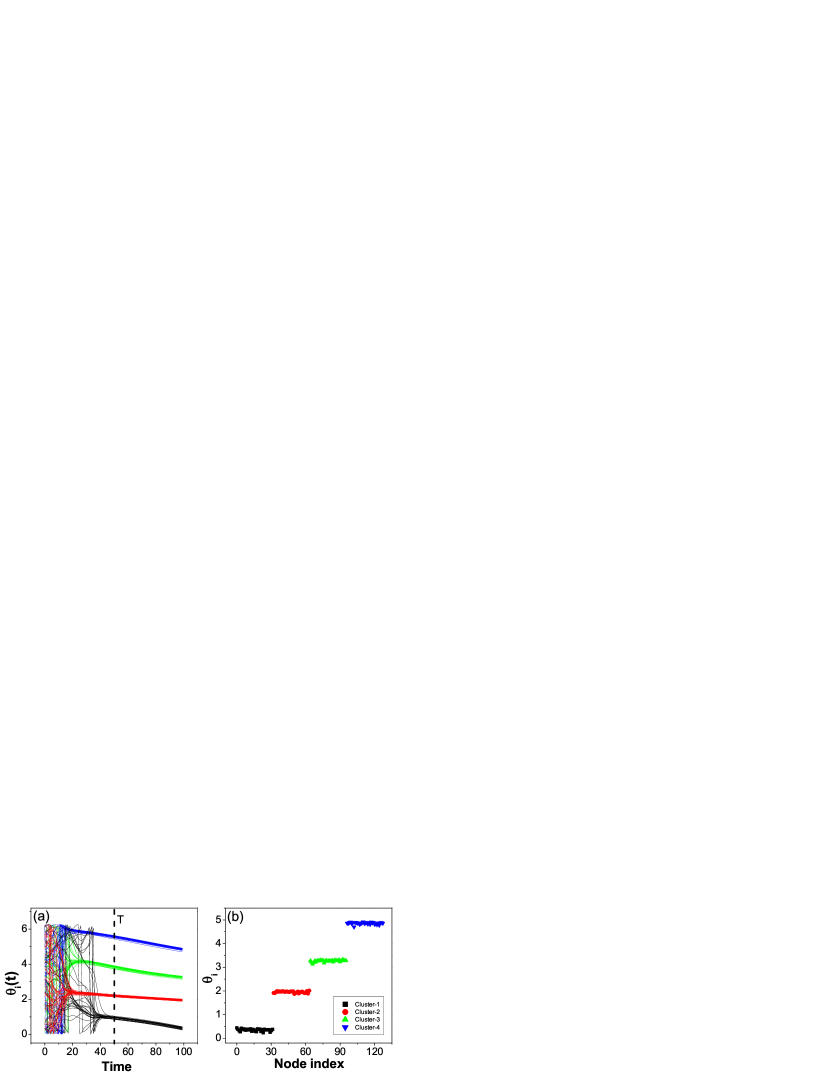
Figure 2: (Color online) For the same network as in Fig. 1, (a) the time evolution of the oscillator states and (b) a snapshot of the oscillator states at time $t=100$.

With the evolution of the subnetworks, the system dynamics is also changed. As shown in Fig. 2(a), with the increase of time, the oscillators are gradually organized into $4$ synchronous clusters. The pattern of the synchronous clusters is more evident in Fig. 2(b), where a snapshot of the oscillator states is taken at time $t=100$. After a check of the node indices of the pattern, it is found that the organization of the dynamical clusters obey precisely the topological clusters. Moreover, in forming the synchronous clusters, it is found that the overlapping nodes, i,e. nodes which have interlinks, are more difficult to be synchronized than those internal nodes. This is clearly evidenced in the synchronizing process of the first cluster, where the few overlapping nodes are traveling among the synchronous clusters for an extra period before settling down (the black curves in Fig. 1(a)). Another interesting finding is that, in the stabilized pattern, the states of the synchronous clusters are well separated from each other, which, of course, is attributed to the repulsive coupling on the interlinks.

A prominent feature of our evolutionary model is that the link functions are updated only by the local network information, i.e., the phase of the local order parameter. While it has been commonly believed that the identification of the link attribute, i.e. intralink or interlink, relies on the knowledge of the global network information, e.g., the betweenness centrality of the network links, it is somewhat surprising to see that here the identification can be accomplished by only the local network information. This interesting phenomenon can be explained by a local mean-field theory, as follows. Let $a_{ij}$ be an intralink of a clustered network. Since nodes inside a cluster are densely connected, nodes $i$ and $j$ thus are surrounded by a similar set of neighboring nodes. Because of the large overlap of their neighboring sets, the average phases $\psi_{i}$ and $\psi_{j}$ will have small difference, leading to the attractive coupling on the intralink, i.e., $e_{ij}=1$. In contrast, if $a_{ij}$ is an interlink, the nodes $i$ and $j$ will be surrounded by very different neighboring sets, which will generate a larger difference in the average phase, finally leading to the repulsive coupling on the interlink.

We next discuss the influences of the network structure on the evolution. Having understood the critical role of the overlapping neighbors in the evolution, we are able to predict that the above phenomena of subnetwork formation can be observed in any network of clear modular structures. To verify this, we have studied the evolution of the other two typical network models. The first one is the overlapping clustered network studied in Ref. LANBHB:2008 , in which two larger clusters (each has $96$ nodes) are mediated by two smaller complete clusters (each has $4$ nodes). The smaller clusters have no direct connection, but each is connected to the two larger clusters by an equal number of links. By analyzing their neighbor sets, the network nodes are immediately classified into four groups: two for the larger clusters and two for the smaller clusters. Correspondingly, the oscillators are expected to be synchronized into $4$ dynamical clusters. This is indeed what we have observed in the simulations [Fig. 3(a) and (b)]. The second model we have simulated is an ER network CN:REV . Since an ER network has no topological cluster, the neighboring sets of the network nodes thus are different from each other. According to the neighbor-set analysis, this will lead to the repulsive couplings on the links, and generating the turbulent system dynamics. This is indeed what we have found at the beginning of the evolution [Fig. 3(c) and (d)]. The repulsive network and turbulent dynamics, however, are unstable. As shown in Fig. 3, after a transient period, the repulsive couplings are quickly switched to the attractive couplings and the turbulent state is changed to the state of global synchronization [Figs. 3(c) and (d)]. The switching of the link functions and system dynamics suggest the dual properties of the ER network, i.e., it can be regarded either as containing no module or as containing one unified module.

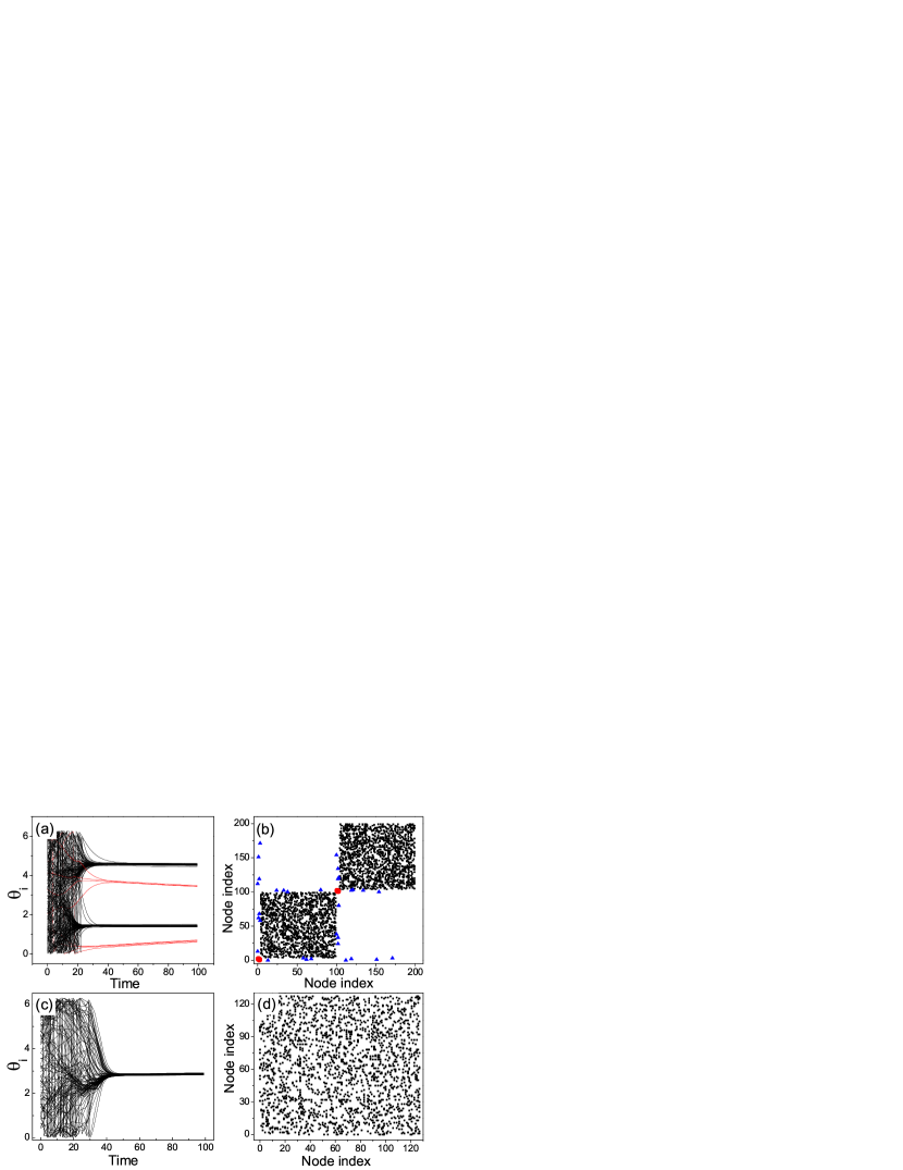
Figure 3: (Color online) For the overlapped clustered network, (a) the evolution of the system dynamics and (b) the stabilized link functions. In (b), the intralinks of the larger and smaller clusters are marked by black squares and red dots, respectively. The interlinks are marked by blue triangles. For a ER network of size $N=128$ and average degree $\left<k\right>=16$, (c) the evolution of the system dynamics and (d) the stabilized link functions. The switching of the link functions and system dynamics are started at about $t=30$. In (d), all network links are granted with the attractive coupling function.

We go on to study the influences of other system parameters on the evolution, including the coupling strength $\varepsilon$, the threshold $D$, and the local dynamics. The numerical results show that, given the network has a clear modular structure, the link attribute can always be successfully detected by the local dynamics, despite the changes of $\varepsilon$ and $D$. Specifically, for the ad hoc network of Fig. 1, the system will always develop to the same functional subnetworks [Fig. 1] and dynamical pattern [Fig. 2] in the parameter space constructed by $\varepsilon\in[0.5,8]$ and $D\in[0.45,\pi/2]$. Furthermore, the main feature of the evolution is independent of the specific form of the local dynamics, as has been verified by other nonlinear oscillators, such as the Logistic map and Lorenz oscillator. However, it should be pointed out that, by changing these parameters, the transient process of the network evolution could be strongly affected, e.g., the transient states of the evolution.

Finally, we discuss the possible application of the evolutionary model in network partition FOOTBALL ; GDGGA:2003 ; RB:2004 ; CNM:2004 ; WL:2008 . In network partition, the performance of an algorithm is mainly measured by the following three factors: ease of implementation, accurate detection and fast computation. All these factors are well met in the evolutionary subnetwork model (ESM). Firstly, on the aspect of ease of implementation, the model employs only the local network information, and the partition is accomplished automatically by the system dynamics. In particular, at the end of the evolution, based on the states of the synchronous clusters, the topological clusters can be readily identified. Automatic detection and local network information are the main features of the ESM algorithm, which are also the major difference to the other dynamics-based algorithms BILPR:2007 ; OCKK:2008 ; RB:2004 . Secondly, the ESM algorithm is fast in computing speed. The computational cost of the ESM method is estimated to be $O(NT)$, with $N$ the network size and $T$ the transient time of the evolution. To estimate the computational cost further, it is necessary to characterize the relationship between $T$ and $N$. Numerically, we have checked this relationship by increasing the size of the ad hoc network in the following two approaches. In the first approach, the number of the clusters are kept unchanged, but the size of the $4$th cluster is gradually increased from $32$ to $864$. In the second approach, the size of each cluster is kept unchanged, but the number of the clusters is increased from $4$ to $30$. The variations of $T$ as a function of $N$ are plotted in Fig. 4(a), together with the synchronizing time, $T^{\prime}$ , of the largest cluster in the network. Very interestingly, it is found that for both approaches we have $T\propto T^{\prime}$. That is, the transient time of the whole network is proportional to that of the largest cluster. Particularly, for the first approach we even have $T\sim T^{\prime}$. Previous studies have indicated that $T^{\prime}$ is mainly determined by the intrinsic properties of the cluster, e.g. the cluster size, instead of the global network properties WHLL:2007 . This implies that $T^{\prime}\sim M_{max}$, with $M_{max}$ the size of the largest cluster in the network. Therefore, the computational cost of ESM is estimated to be proportional to $O(NM_{max})$. Since for practical networks we generally have $M_{max}\ll N$, the computational cost of ESM thus is estimated to increase linearly with the network size. Finally, on the aspect of detecting accuracy, the ESM algorithm works very well for clustered networks and reasonably well for fuzzy networks [Fig. 4(b)].

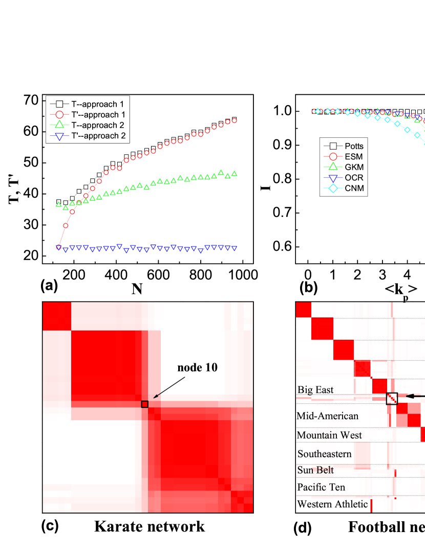
Figure 4: (Color online) For the ad hoc network of Fig. 1, (a) the transient time of the whole network, $T$, and the synchronizing time of the largest cluster in the nework, $T^{\prime}$, as a function of the network size, and (b) the variation of the mutual information (see Ref. DGDA:2005 for details about mutual information) as a function of $\left<k_{p}\right>$ generated by the partition algorithms “Potts” RB:2004 , “ESM”, “GKM” OCKK:2008 , “OCR” BILPR:2007 , and “CNM” CNM:2004 . The coappearance matrix generated by ESM for (c) the Zachary’s karate club and (d) the football club. The overlapping nodes are marked by the squares. In (c) and (d), each data is averaged over $100$ realizations.

As applications of the new algorithm, we have tested the partitions of two empirical clustered networks. The first one is the Zachary’s karate club network KARATE , which contains $34$ nodes and $78$ links. The numerical result is plotted in Fig. 4(c), in which the network is clearly divided into $4$ clusters. Moreover, the overlapping node, i.e. the $10$th node in the network, is also well characterized. These results coincide with that of Ref. KARATE . The second example we have tested is the football network FOOTBALL , which contains $115$ nodes (teams) and $613$ (matches) links. The numerical result is plotted in Fig. 4(d), in which the network is clearly divided into a number of conferences (clusters). Again, the independent teams, which have equal number of games (links) with multiple conferences, are well identified by the overlapping nodes. These results coincide with that of Ref. FOOTBALL .

In summary, we have studied the evolution of functional subnetworks in clustered networks and proposed a new algorithm for partitioning networks. Hopefully, the finding that the network function is jointly determined by the network structure and system dynamics could be helpful to the study of complex behaviors in functional networks.

References

- (1) R. Albert and A.-L. Barabási, Rev. Mod. Phys. 74, 47 (2002); M.E.J. Newman, SIAM Rev. 45, 167 (2003).
- (2) S. Boccaletti, et.al., Phys. Rep. 424, 175 (2006); A. Arenas, et.al., Phys. Rep. 469, 93 (2008).
- (3) X. F. Wang and G. Chen, Int. J. Bifurcation Chaos Appl. Sci. Eng. 12, 187 (2002); M. Barahona and L. M. Pecora, Phys. Rev. Lett. 89, 054101 (2002); T. Nishikawa, et.al., Phys. Rev. Lett. 91, 014101 (2003); X. G. Wang, et.al., Phys. Rev. E 75, 056205 (2007); A. Arenas, Phys. Rev. Lett. 98, 034101 (2007).
- (4) I.V. Belykh, et.al., Physica D 195, 188 (2004); W. Li, et.al., Phys. Rev. E 76, 045102(R) (2007).
- (5) P. Gong, C.V. Leeuwen, Europhys. Lett. 67, 328 (2004).
- (6) A. Arenas, et.al., Phys. Rev. Lett. 96, 114102, (2006)
- (7) C. Zhou and J. Kurths, Phys. Rev. Lett. 96, 164102 (2006).
- (8) S. Boccaletti, et.al., Phys. Rev. E 75, 045102(R) (2007).
- (9) E. Oh, et.al., Europhys. Lett. 83, 68003 (2008).
- (10) D. Li, et.al., Phys. Rev. Lett. 101, 168701 (2008).
- (11) C.S. Zhou, et.al., Phys. Rev. Lett. 97, 238103 (2006).
- (12) D. Purves and J. Lichtman, Principles of Neural Development (Sinauer Associates, Sunderland, MA, 1985).
- (13) J. Hofbauer and K. Sigmund, Evolutionary Games and Population Dynamics (Cambridge University Press, Cambridge, 1998).
- (14) J. G. Restrepo, et.al., Phys. Rev. E 71, 036151 (2005); X.G. Wang, et.al., Chaos 18, 037117 (2008).
- (15) M. Girvan and M.E.J. Newman, Proc. Natl. Acad. Sci. USA 99, 7821 (2002).
- (16) R. Guimerá, et.al., Phys. Rev. E 68, 065103(R), (2003); J. Duch and A. Arenas, Phys. Rev. E 72, 027104, (2005);
- (17) J. Reichardt and S. Bornholdt, Phys. Rev. Lett. 93, 218701 (2004).
- (18) A. Clauset, et.al., Phys. Rev. E 70, 066111 (2004).
- (19) J. Wang, C.-H. Lai, New J. Phys. 10, 123023 (2008).
- (20) L. Danon, et.al., J. Stat. Mech. P09008 (2005).
- (21) X.G. Wang, et.al., Phys. Rev. E 76, 056113 (2007).
- (22) W.W. Zachary, J. Anthropol. Res. 33,452 (1977).