Cosmological Radiation Hydrodynamics with Enzo

Abstract

We describe an extension of the cosmological hydrodynamics code Enzo to include the self-consistent transport of ionizing radiation modeled in the flux-limited diffusion approximation. A novel feature of our algorithm is a coupled implicit solution of radiation transport, ionization kinetics, and gas photoheating, making the timestepping for this portion of the calculation resolution independent. The implicit system is coupled to the explicit cosmological hydrodynamics through operator splitting and solved with scalable multigrid methods. We summarize the numerical method, present a verification test on cosmological Strömgren spheres, and then apply it to the problem of cosmological hydrogen reionization.

1 Introduction

It is a distinct privilege to help celebrate Dimitri Mihalas’ 70th birthday by reporting on our latest work at this Festschrift in his honor. As a former faculty colleague of his at UIUC and scientific collaborator, I could tell many anecdotes. However of the many things I learned from Dimitri, the two that stick with me are: (1) solve the problem you need to solve to do the science, and (2) be rigorous about how you do it. These lessons motivate our present approach to self-consistent cosmological radiation hydrodynamics which is documented more fully in Reynolds et al. (2009).

A current frontier in cosmological structure formation simulations is including the feedback of radiating sources such as galaxies and AGN on the intergalactic medium (IGM) in a self-consistent way. For example, the collective UV radiation from protogalaxies is believed to reionize the IGM at $z\approx 7-8$ Fan et al. (2006). This process can be thought of as the expansion and eventual overlap of R-type ionization fronts driven by high rates of star formation in the protogalaxies. R-type ionization fronts couple to the gas very weakly. Consequently a number of studies have simulated cosmological reionization by post-processing density fields taken from cosmological simulations with a standalone radiative transfer code ; e.g. Ciardi et al. (2003); Sokasian et al. (2004); Iliev et al. (2006). However, closer to the sources and within the galaxies themselves where the gas density is higher, or when an intergalactic R-type front sweeps over a dense clump, ionization fronts may become D-type. When this happens coupling to gas motions is strong and a self-consistent approach to modeling is required in which hydrodynamics, radiative transfer, and the thermal/ionization state of the gas are evolved in a coupled fashion Whalen and Norman (2006).

Iliev et al. (2009) summarizes a variety of methods currently under development by the numerical cosmology community that do this. The radiative transfer methods employed include ray tracing, Monte Carlo, and moment methods. Here we present a method based on flux-limited diffusion. A novel feature of our algorithm is a coupled implicit solution of radiation transport, ionization kinetics, and gas photoheating, making the timestepping for this portion of the calculation resolution independent. This will be essential when adaptive mesh refinement (AMR) is employed. At present our algorithm is only implemented on uniform (non-adaptive) Cartesian grids. After describing our method, we verify its correctness on a cosmological Strömgren sphere test problem. We then present a low-resolution “first light” test of the coupled code to the problem of cosmological reionization. A more comprehensive description of our method and verification tests can be found in Reynolds et al. (2009).

2 Physical Model

We consider the coupled system of partial differential equations

$$\partial_{t}\rho_{b}+\frac{1}{a}{\bf v}_{b}\cdot\nabla\rho_{b} =-\frac{1}{a}\rho_{b}\nabla\cdot{\bf v}_{b},$$ (1)

$$\partial_{t}{\bf v}_{b}+\frac{1}{a}\left({\bf v}_{b}\cdot\nabla\right){\bf v}_{b} =-\frac{\dot{a}}{a}{\bf v}_{b}-\frac{1}{a\rho_{b}}\nabla p-\frac{1}{a}\nabla\phi,$$ (2)

$$\partial_{t}e+\frac{1}{a}{\bf v}_{b}\cdot\nabla e =-\frac{2\dot{a}}{a}e-\frac{1}{a\rho_{b}}\nabla\cdot\left(p{\bf v}_{b}\right)-\frac{1}{a}{\bf v}_{b}\cdot\nabla\phi+G-\Lambda$$ (3)

$$\partial_{t}{\tt n}_{i}+\frac{1}{a}\nabla\cdot\left({\tt n}_{i}{\bf v}_{b}\right) =\alpha_{i,j}{\tt n}_{e}{\tt n}_{j}-{\tt n}_{i}\Gamma_{i}^{ph},\qquad i=1,\ldots,N_{s},$$ (4)

$$\partial_{t}E+\frac{1}{a}\nabla\cdot\left(E{\bf v}_{b}\right) =\nabla\cdot\left(D\nabla E\right)-\frac{\dot{a}}{a}E+4\pi\eta-c\kappa E,$$ (5)

$$\nabla^{2}\phi =\frac{4\pi g}{a}(\rho_{b}+\rho_{dm}-\langle\rho\rangle).$$ (6)

These describe conservation of mass (1), conservation of momentum (2), conservation of energy (3), chemical rate equations (4), flux-limited diffusion radiative transfer (5) and Poisson’s equation (6), in a coordinate system that is comoving with the expanding universe Bryan et al. (1995); Hayes and Norman (2003); Paschos (2005); Reynolds et al. (2009). The independent variables in these equations consist of the comoving baryonic density $\rho_{b}$, the proper peculiar baryonic velocity ${\bf v}_{b}$, the total gas energy per unit mass $e$, the comoving number density for each chemical species ${\tt n}_{i},\;i=1,\ldots,N_{s}$, the comoving radiation energy density $E$, and the modified gravitational potential $\phi$.

The cosmological flux-limited diffusion (FLD) equation (5) deserves some comment. In deriving this equation from the general multi-frequency version Paschos (2005),

$$\partial_{t}E_{\nu}+\frac{1}{a}\nabla\cdot(E_{\nu}{\bf v}_{b})=\nabla\cdot(D\,\nabla E_{\nu})+\nu\frac{\dot{a}}{a}\partial_{\nu}E_{\nu}+4\pi\eta_{\nu}-c\kappa_{\nu}E_{\nu},$$ (7)

we have assumed a prescribed radiation frequency spectrum, $\chi_{E}(\nu)$, allowing the frequency-dependent radiation energy density to be written in the form $E_{\nu}({\bf x},t,\nu)=\tilde{E}({\bf x},t)\,\chi_{E}(\nu)$. With this assumption, the single “grey” radiation energy density is given by

$$E({\bf x},t)=\int_{\nu_{0}}^{\infty}E_{\nu}({\bf x},t,\nu)d\nu=\tilde{E}({\bf x},t)\int_{\nu_{0}}^{\infty}\chi_{E}(\nu)d\nu,$$ (8)

and the equation (5) is then obtained through integration of (7) over frequencies ranging from the ionization threshold of hydrogen ($h\nu_{0}=13.6$ eV) to infinity. In this paper we assume the radiation has a $T_{B}=10^{5}$ blackbody spectrum, i.e. $\chi_{E}(\nu)=8\pi h\left(\frac{\nu}{c}\right)^{3}\big{/}\left(\exp\left(\frac{h\nu}{k_{b}T_{B}}\right)-1\right)$.

The dependent variables in these equations are the proper pressure $p$, the temperature $T$, and the comoving electron number density ${\tt n}_{e}$, given through the equations

$$p =\rho_{b}(\gamma-1)\left(e-\frac{1}{2}|{\bf v}_{b}|^{2}\right),$$ (9)

$$T =(\gamma-1)\frac{p\,\mu\,m_{p}}{\rho_{b}\,k_{b}},$$ (10)

$${\tt n}_{e} =\begin{cases}{\tt n}_{HII},&\text{(hydrogen only)}\\ {\tt n}_{HII}+\tfrac{1}{4}{\tt n}_{HeII}+\tfrac{1}{2}{\tt n}_{HeIII},&\text{(hydrogen + helium)}.\end{cases}$$ (11)

Here $\gamma$ is the ratio of specific heats, which we take to be $5/3$; $m_{p}$ corresponds to the mass of a proton and $k_{b}$ is Boltzmann’s constant. The local molecular weight $\mu$ depends on the density and chemical ionization state.

In addition, the system (1)-(6) contains a number of coupling terms and coefficients. The coefficient $a(t)\equiv(1+z)^{-1}$ denotes the cosmological expansion parameter for a smooth homogeneous background, where the redshift $z$ is a function of time only; all spatial derivatives are therefore taken with respect to the comoving position ${\bf x}\equiv{\bf r}/a(t)$. The term $\dot{a}=\frac{\mathrm{d}a(t)}{\mathrm{d}t}$. $a(t)$ is obtained by integrating the Friedmann equation for the set of assumed cosmological parameters. The gas heating and cooling rates $G$ and $\Lambda$ are functions of the temperature, radiation energy density and chemical ionization state. The temperature-dependent chemical reaction rates $\alpha_{i,j}$ define the interactions between chemical species, and the photoionization rate $\Gamma_{i}^{ph}$ depends on the radiation energy density. Formulas for all of these terms may be found in the references Black (1981); Osterbrock (1989); Cen (1992); Abel et al. (1997); Hui and Gnedin (1997); Razoumov et al. (2002).

In the radiation equation (5), $c$ is the speed of light, the total opacity $\kappa$ is a function of the chemical ionization state, and the emissivity $\eta$ is provided as either a radiation source term, or may depend on the density, velocity, gas energy, and chemical ionization state. The formulae for these dependencies may be found in the references Osterbrock (1989); Cen and Ostriker (1992). Of special importance in this equation is the coefficient function $D$, which in a flux-limited diffusion approximation attempts to allow the equation to span behaviors ranging from nearly isotropic to free-streaming radiation. To this end, we choose the coefficient to be of the form

$$D(E)=\text{diag}\left(D_{1}(E),D_{2}(E),D_{3}(E)\right),\quad\text{where}\quad D_{i}(E)=\frac{c(2\kappa_{T}+R_{i})}{6\kappa_{T}^{2}+3\kappa_{T}R_{i}+R_{i}^{2}},$$ (12)

with $R_{i}=|\partial_{i}E|/E,\,i=1,2,3$. Here $\kappa_{T}=\kappa+\kappa_{S}$ is the total extinction coefficient, where $\kappa$ is the opacity and $\kappa_{S}$ results from scattering Hayes et al. (2006). The function (12) has been reformulated from its original version Hayes and Norman (2003) to provide increased stability for scattering-free simulations involving extremely small opacities (i.e. $\kappa_{T}=\kappa\ll 1$), as is typical in cosmology applications.

In the Poisson equation for the gravitational potential (6), the baryonic gas is coupled to collisionless dark matter $\rho_{dm}$ and the cosmic mean density $\langle\rho\rangle$ solely through their self–consistent gravitational field. Here, $g$ provides the gravitational constant, and the dark matter density is evolved using the Particle-Mesh method described in Hockney and Eastwood (1988); Norman and Bryan (1999); O’Shea et al. (2004).

3 Algorithm

Instead of working with the equations directly in CGS units, we first normalize the system to render the values tractable for floating point computation. To this end, we define the scaled units

$$\tilde{x}=x/u_{x},\qquad\tilde{g}=g/u_{g},\qquad\tilde{t}=t/u_{t},$$ (13)

where the constants $u_{x}$, $u_{t}$ and $u_{g}$ correspond to the typical magnitudes of length, time and mass at the start of the simulation. We further define the density unit factor $u_{d}=u_{g}/(u_{x})^{3}$ and velocity scaling factor $u_{v}=u_{x}/u_{t}$. We note that due to our use of comoving length, these constants are all redshift-independent. The proper length values at any point in the simulation are therefore given by

$$x_{\text{proper}}=x\,a(t)=\tilde{x}\,u_{x}\,a(t).$$ (14)

With these unit scalings, we define the normalized variables

$$\tilde{\rho}_{b}=\rho/u_{d}, \qquad\tilde{\bf v}_{b}={\bf v}_{b}/u_{v},\qquad\tilde{e}=e/u_{v}^{2},$$ (15)

$$\tilde{E}=E/\left(u_{d}u_{v}^{2}\right), \qquad\tilde{{\tt n}}_{i}={\tt n}_{i}/u_{d},\qquad\tilde{\phi}=\phi/u_{v}^{2}.$$

The proper densities may be obtained from the comoving densities through the formulae

$$E_{\text{proper}} =E/a^{3}(t)=\tilde{E}\frac{u_{E}}{a^{3}(t)},$$

$${\tt n}_{i,{\text{proper}}} ={\tt n}_{i}/a^{3}(t)=\tilde{{\tt n}}_{i}\frac{u_{n}}{a^{3}(t)},$$ (16)

$$\rho_{b,\text{proper}} =\rho_{b}/a^{3}(t)=\tilde{\rho}_{b}\frac{u_{n}}{a^{3}(t)}.$$

With these rescaled variables, we rewrite our equations (1)-(6) as the normalized system

$$\partial_{\tilde{t}}\tilde{\rho}_{b}+\frac{1}{a}\tilde{\bf v}_{b}\cdot\tilde{\nabla}\tilde{\rho}_{b} =-\frac{1}{a}\tilde{\rho}_{b}\tilde{\nabla}\cdot\tilde{\bf v}_{b},$$ (17)

$$\partial_{\tilde{t}}\tilde{\bf v}_{b}+\frac{1}{a}\left(\tilde{\bf v}_{b}\cdot\tilde{\nabla}\right)\tilde{\bf v}_{b} =-\frac{\dot{a}}{a}\tilde{\bf v}_{b}-\frac{1}{a\tilde{\rho}_{b}}\tilde{\nabla}\tilde{p}-\frac{1}{a}\tilde{\nabla}\tilde{\phi},$$ (18)

$$\partial_{\tilde{t}}\tilde{e}+\frac{1}{a}\tilde{\bf v}_{b}\cdot\tilde{\nabla}\tilde{e} =-\frac{2\dot{a}}{a}\tilde{e}-\frac{1}{a\tilde{\rho}_{b}}\tilde{\nabla}\cdot\left(\tilde{p}\tilde{\bf v}_{b}\right)-\frac{1}{a}\tilde{\bf v}_{b}\cdot\tilde{\nabla}\tilde{\phi}+\tilde{G}-\tilde{\Lambda}$$ (19)

$$\partial_{\tilde{t}}\tilde{{\tt n}}_{i}+\frac{1}{a}\tilde{\nabla}\cdot\left(\tilde{{\tt n}}_{i}\tilde{\bf v}_{b}\right) =\tilde{\alpha}_{i,j}{\tt n}_{e}\tilde{{\tt n}}_{j}-\tilde{{\tt n}}_{i}\tilde{\Gamma}_{i}^{ph},\qquad i=1,\ldots,N_{s},$$ (20)

$$\partial_{\tilde{t}}\tilde{E}+\frac{1}{a}\tilde{\nabla}\cdot\left(\tilde{E}\tilde{\bf v}_{b}\right) =\tilde{\nabla}\cdot\left(D\tilde{\nabla}\tilde{E}\right)-\frac{\dot{a}}{a}\tilde{E}+4\pi\tilde{\eta}-c\tilde{\kappa}\tilde{E},$$ (21)

$$\tilde{\nabla}^{2}\tilde{\phi} =\frac{4\pi\tilde{g}}{a}(\tilde{\rho}_{b}+\tilde{\rho}_{dm}-\langle\tilde{\rho}\rangle).$$ (22)

Here, $\dot{a}$ now refers to the derivative $\frac{\mathrm{d}a}{\mathrm{d}\tilde{t}}$. For clarity of notation, all subsequent variables are shown without the $\sim$ superscript, although all solver algorithms operate on the normalized variables.

3.1 Operator-Split Hydrodynamics with Radiative Feedback

We solve the coupled system (17)-(22) using an operator-split framework, wherein we solve sub-components of the system one at a time, feeding the results of each sub-system into the remaining parts. In this approach, a time step is taken with the steps:

• Project the dark matter particles onto the finite-volume mesh to generate the dark matter density field $\rho_{dm}$.

• Solve for the gravitational potential $\phi$ using equation (22).

• Advect the dark matter particles with the Particle-Mesh method Hockney and Eastwood (1988); Norman and Bryan (1999); O’Shea et al. (2004).

• Evolve the hydrodynamics equations (17)-(19) with a high-order, explicit-time upwind method. In this step, the velocity field ${\bf v}_{b}$ advects both the chemical number densities ${\tt n}_{i}$ and radiation energy density $E$.

• Using a high-order implicit method, solve a coupled reaction-diffusion system (19)-(21) to obtain the updated number densities ${\tt n}_{i}$, radiation $E$ and gas energy $e$.

The equation (19) is involved in both steps (iv) and (v) above. To do this, we split the gas energy into two parts, $e=e_{h}+e_{c}$, where $e_{h}$ results from the hydrodynamic evolution of the system (step (iv)), and $e_{c}$ is the gas energy correction that results from couplings with radiation and chemistry (step (v)). With this splitting, the hydrodynamic solver used in step (iv) of the algorithm solves the system of equations

$$\partial_{t}\rho_{b}+\frac{1}{a}{\bf v}_{b}\cdot\nabla\rho_{b} =-\frac{1}{a}\rho_{b}\nabla\cdot{\bf v}_{b},$$ (23)

$$\partial_{t}{\bf v}_{b}+\frac{1}{a}\left({\bf v}_{b}\cdot\nabla\right){\bf v}_{b} =-\frac{\dot{a}}{a}{\bf v}_{b}-\frac{1}{a\rho_{b}}\nabla p-\frac{1}{a}\nabla\phi,$$ (24)

$$\partial_{t}e_{h}+\frac{1}{a}{\bf v}_{b}\cdot\nabla e_{h} =-\frac{2\dot{a}}{a}e_{h}-\frac{1}{a\rho_{b}}\nabla\cdot\left(p{\bf v}_{b}\right)-\frac{1}{a}{\bf v}_{b}\cdot\nabla\phi$$ (25)

$$\partial_{t}{\tt n}_{i}+\frac{1}{a}\nabla\cdot\left({\tt n}_{i}{\bf v}_{b}\right) =0,$$ (26)

$$\partial_{t}E+\frac{1}{a}\nabla\cdot\left(E{\bf v}_{b}\right) =0,$$ (27)

using the Piecewise Parabolic Method (PPM) Colella and Woodward (1984), on a regular finite-volume spatial grid. This solve evolves $(\rho_{b}^{n},{\bf v}_{b}^{n},e^{n},{\tt n}_{i}^{n},E^{n})$ to the time-updated variables $(\rho_{b}^{n+1},{\bf v}_{b}^{n+1},e_{h}^{n+1})$ and the advected variables $({\tt n}_{i}^{*},E^{*})$, and is implemented in the community astrophysics code Enzo O’Shea et al. (2004); Norman et al. (2007); enz (????).

Step (v) then solves the coupled system,

$$\partial_{t}e_{c} =-\frac{2\dot{a}}{a}e_{c}+G-\Lambda,$$ (28)

$$\partial_{t}{\tt n}_{i} =\alpha_{i,j}{\tt n}_{e}{\tt n}_{j}-{\tt n}_{i}\Gamma_{i}^{ph},$$ (29)

$$\partial_{t}E =\nabla\cdot\left(D\nabla E\right)-m\frac{\dot{a}}{a}E+4\pi\eta-c\kappa E,$$ (30)

using a fully implicit nonlinear solution approach to evolve the advected variables $(e_{c}^{n},{\tt n}_{i}^{*},E^{*})$ to the time-evolved quantities $(e_{c}^{n+1},{\tt n}_{i}^{n+1},E^{n+1})$. To this end, we define the vector of unknowns $U=(e_{c},{\tt n}_{i},E)^{T}$, and write the nonlinear residual function $f(U)=(f_{e},f_{{\tt n}_{i}},f_{E})^{T}$, where

$$f_{e}(U)\ \equiv\ e_{c}-S_{e}(U),$$ (31)

$$f_{{\tt n}_{i}}(U)\ \equiv\ {\tt n}_{i}-S_{{\tt n}_{i}}(U),\quad i=1,\ldots,N_{s},$$ (32)

$$f_{E}(U)\ \equiv\ E-E^{n}-\Delta t\,\theta\left(\nabla\cdot\left(D\nabla E\right)-\frac{\dot{a}}{a}E+4\pi\eta-ckE\right)$$ (33)

$$-\Delta t(1-\theta)\left(\nabla\cdot\left(D^{n}\nabla E^{n}\right)-\frac{\dot{a}}{a}E^{n}+4\pi\eta^{n}-ck^{n}E^{n}\right),$$

Here the functions $S_{e}(U)$ and $S_{{\tt n}_{i}}(U)$ provide the analytical solutions to an $O(\Delta t^{2})$-accurate approximation of the spatially-local ODE system (28)-(29) for a given value of $E$ Reynolds (2009). The residual equation (33) defines a standard two-level $\theta$ method for time integration of the equation (30). Therefore this overall nonlinear residual defines an up-to-second order implicit time discretization of the coupled system (28)-(30); where the time-evolved state $U^{n+1}$ is found through solution of the problem $f(U)=0$.

To solve this nonlinear problem, we use a globalized Inexact Newton’s Method Kelley (1995); Knoll and Keyes (2004), that iteratively proceeds toward the solution $U^{n+1}$ through approximately solving a sequence of linearized problems $J(U_{k})S_{k}=-f(U_{k})$, where $J(U_{k})$ is the Jacobian of the nonlinear function $f$, evaluated at the current Newton iterate $U_{k}$. A full description of our solution algorithm is provided in Reynolds et al. (2009). To summarize this process, we solve these linear Newton systems through a Schur complement formulation, that reduces the coupled linear system to a sequence of simpler sub-systems, culminating in an update to a modified radiation equation. This Schur complement subsystem is solved using a multigrid-preconditioned conjugate gradient method from the HYPRE library Falgout and Yang (2002); hyp (????); Baker et al. (2006).

We measure convergence of the Newton iteration with the RMS norm

$$\|w\|=\left(\frac{\|w\|_{2}^{2}}{N(N_{s}+2)}\right)^{1/2},$$ (34)

where $N(N_{s}+2)$ is the number of unknowns in $w$, since this norm does not grow artificially larger with mesh refinement.

4 Verification tests

The model equations and solution algorithm in this paper have been rigorously tested on a myriad of problems, ranging from pure radiation transport, to interacting radiation and hydrodynamics, to dynamic radiation-hydrodynamics with chemical ionization Reynolds et al. (2009). In lieu of reiterating those tests here, we demonstrate the approach on a single problem before moving on to our target application.

We consider a verification problem that performs isothermal ionization of a static (i.e., no fluid motions other than Hubble expansion) neutral hydrogen region, within a cosmologically expanding universe. The problem is originally due to Shapiro & Giroux Shapiro and Giroux (1987), and exercises the radiation transfer, cosmology and chemical ionization components of the coupled solver. The physics of interest in this example is the expansion of an ionized hydrogen region in a uniform gas around a single monochromatic source, emitting $\dot{N}_{\gamma}=5\times 10^{48}$ photons per second at the ionization frequency of hydrogen ($h\nu=13.6$ eV). Given the initially-neutral hydrogen region and strength of the ionizing source, the ionization region expands rapidly at first, with the I-front approaching the equilibrium position where ionizations and recombinations balance, referred to as the Strömgren radius. However, due to cosmological expansion, this equilibrium radius begins to increase much faster than the I-front can propagate. The analytical formula for the location of the Strömgren radius as a function of time is

$$r_{S}(t)=\left[\frac{3\dot{N}_{\gamma}}{4\pi\alpha_{B}{\tt n}_{H}(t)^{2}}\right]^{1/3},$$ (35)

where the proper hydrogen number density ${\tt n}_{H}$ decreases due to cosmological expansion by a factor of $a^{-3}(t)$. Here $\alpha_{B}\approx 2.59\times 10^{-13}$ cm³/s is the case-B hydrogen recombination coefficient. If we define $\lambda=\alpha_{B}{\tt n}_{H,0}/H_{0}/(1+z_{0})$, where ${\tt n}_{H,0}$ is the hydrogen number density at the initial redshift $z_{0}$, we may calculate the analytical I-front radius at any point in time as

$$r_{I}(t) =r_{S,0}\left(\lambda\,e^{-\tau(t)}\int_{1}^{a(t)}e^{\tau(\tilde{a})}\left[1-2q_{0}+2q_{0}(1+z_{0})/\tilde{a}\right]^{-1/2}\mathrm{d}\tilde{a}\right)^{1/3},$$ (36)

where

$$\tau(a) =\lambda\,\left[6\,q_{0}^{2}\,(1+z_{0})^{2}\right]^{-1}\left[F(a)-F(1)\right],$$ (37)

$$F(a) =\left[2-4q_{0}-2q_{0}(1+z_{0})/a\right]\left[1-2q_{0}+2q_{0}(1+z_{0})/a\right]^{1/2},$$ (38)

and where $q_{0}$ is the cosmological deceleration parameter.

We perform four of the tests provided in the original paper Shapiro and Giroux (1987): $q_{0}=\{0.5,0.05\}$, and $z_{0}=\{4,10\}$. These correspond to the cosmological parameters found in Table 1.

$q_{0}$	$z_{0}$	$L_{0}$	$H_{0}$	$\Omega_{m}$	$\Omega_{\Lambda}$	$\Omega_{b}$
0.5	4	80 kpc	0.5	1.0	0	0.2
0.05	4	60 kpc	1.0	0.1	0	0.1
0.5	10	36 kpc	0.5	1.0	0	0.2
0.05	10	27 kpc	1.0	0.1	0	0.1

Table 1: Cosmological parameters for the verification tests. See text for descriptions.

Here, $L_{0}$ is the initial box size and $H_{0}$ is the Hubble constant. The values $\Omega_{m}$, $\Omega_{\Lambda}$ and $\Omega_{b}$ are the contributions to the gas energy density at $z=0$ due to non-relativistic matter, the cosmological constant, and baryonic matter, respectively. These two deceleration parameters result in slightly different functions for the expansion coefficient $a$. For $q_{0}=0.05$ we compute $a(t)$ using equations (13-3) and (13-10) from Peebles (1993), while for $q_{0}=0.5$ we compute $a(t)=(1+z(t))^{-1}$. We begin all problems with an initial radiation energy density of $E=10^{-35}$ erg cm^-3 and an initial ionization fraction $n_{HII}/{\tt n}_{H,0}=0$. The initial density is chosen as $\rho_{b,0}=1.175\times 10^{-28}$ g cm^-3 for $q_{0}=0.5$, or $\rho_{b,0}=2.35\times 10^{-28}$ g cm^-3 for $q_{0}=0.05$. All simulations are run from the initial redshift $z_{0}$ to $z=0$. The ionization source is located in the lower corner of the box. We use reflecting boundary conditions at the lower boundaries and outflow conditions at the upper boundaries in each direction. The implicit solver used a convergence norm of $p=2$, time step parameter of $\theta=0.51$, a desired temporal solution accuracy $\tau_{\text{tol}}=0.001$ and inexactness parameter $\delta_{k}=10^{-13}\|f(U_{k})\|$ (see Reynolds et al. (2009) for further explanation of these parameters).

In Figure 1 we plot the scaled, spherically-averaged I-front position with respect to scaled redshift for each of the four tests (with axes identical to Shapiro and Giroux (1987), Figure 1a), as well as the zoomed-in version for the $z_{0}=4$ tests along with their analytical solutions; all of these tests used a $128^{3}$ spatial mesh.

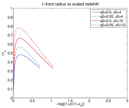
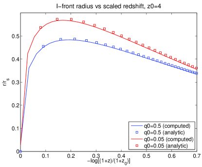
Figure 1: Left: I-front radius vs. scaled redshift for the four tests. Right: I-front radius vs scaled redshift for the $z_{0}=4$ tests; analytical solution values are shown with open squares.

In Figure 2 we plot the error in the computed I-front radius as we varied the spatial mesh size for the two cases $(q_{0},z_{q})=(0.5,4)$ and $(0.05,4)$. The accuracy in the computed radius improves with mesh refinement.

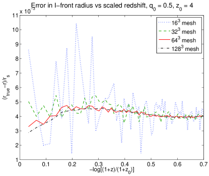
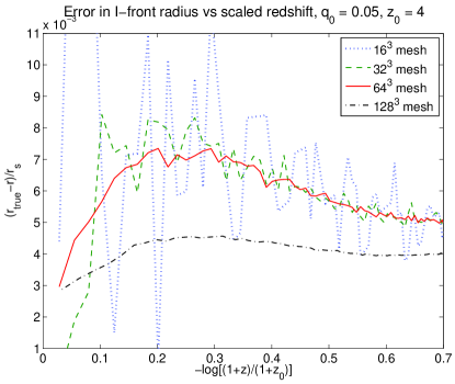
Figure 2: Convergence of I-front radius vs. scaled redshift for the cases $q_{0}=\{0.5,0.05\}$ and $z_{0}=4$ as the mesh is refined: spatial meshes shown are $16^{3}$ (blue dotted), $32^{3}$ (green dashed), $64^{3}$ (red solid), and $128^{3}$ (black dot-dashed).

5 Application to cosmological reionization

To illustrate the operation of the combined cosmological radiation hydrodynamics plus ionization kinetics code, we simulate hydrogen reionization due to stellar sources in a small cosmological volume. This is a low resolution functionality test only to show that the two halves of the code are coupled correctly; scientific predictions will require considerably higher resolution and larger boxes Trac et al. (2008).

We simulate a $\Lambda$CDM cosmological model with the following parameters: $\Omega_{\Lambda}=0.7$, $\Omega_{b}=0.04$, $\Omega_{CDM}=0.26$, $h=0.7$, $\sigma_{8}=0.9$, where these are, respectively, the fraction of the closure density in vacuum energy, baryons, and cold dark matter, the Hubble constant in units of 100 km/s/Mpc, and the variance of matter fluctuations in 8 Mpc^-1 spheres, all measured at the present epoch (z=0). A Gaussian random field is initialized at z=99 using an initial power spectrum following Eisenstein and Hu (1999). The simulation was run in an 8 Mpc comoving box using a $64^{3}$ uniform grid and dark matter particles with periodic boundary conditions.

The emissivity $\eta$ was computed using a modified version of the star formation/feedback recipe of Cen and Ostriker (1992), in which the conditions for star formation within a computational cell require that the local ${\bf v}_{b}$ have negative divergence (i.e baryons are contracting), the radiative cooling time is smaller than the dynamical time, and that $\rho_{b}$ is greater than some threshold (without checking for the Jeans mass). If these criteria are met a star particle is created which represents an ensemble of stars and becomes a source of emissivity for the radiation solver. Many particles are created over time and there may be multiple star particles in a cell. The emissivity of a cell $\eta$ is computed as follows:

$$\eta=\frac{1}{4\pi}\sum\limits_{i}\,\epsilon_{UV}\int_{t}^{t+\Delta t}\dot{m}_{SF}(t)\,c^{2}\,\mathrm{d}t$$ (39)

where the sum is over all the star particles in the cell, $\dot{m}_{SF}(t)$ is the star formation rate, which is an assumed analytic function of time for each particle, $c$ is the speed of light, $\Delta t$ is the timestep, and $\epsilon_{UV}$ an efficiency factor that depends on a number of hidden parameters including the initial mass function of the star cluster, the stellar spectral energy distribution, and the ionizing photon escape fraction. For simplicity, we used the upper value from Razoumov et al. (2002) in its place.

Snapshots from the simulation are created by the analysis tool yt Turk (2008) and shown in Table 2. Here projections through the three dimensional volume are shown for four redshifts $z$ = 4.35, 2.55, 1.99 and 0 and three physical quantities: baryonic density ($\log_{10}(\rho_{b}/\rho_{avg})$), ionization fraction ($\log_{10}({\tt n}_{HII}/{\tt n}_{H})$) and temperature ($\log_{10}T$) in Kelvin.

The first star particle was created at $z=5.58$. At this point, the initially homogeneous Intergalactic Medium (IGM) had formed filamentry structures as a result of dark matter clumps. By the first snapshot at $z=4.35$, the effects of the star can clearly be seen in the higher ionization fraction in the lower right corner region around the star. This same region is evident by a brighter peak in the density and temperature.

Table 2: Cosmological ionization snapshots: 2D data results from averaging through one direction. The rows correspond to times $z$ = 4.35, 2.55, 1.99, 0; the columns show baryonic density, ionization fraction and temperature.

By $z=2.55$, multiple sources have formed and are contributing to the ionizing radiation. The ionization fronts have also clearly propagated through significantly more of the domain. Although the ionization fronts are converging, there are still small pockets where the IGM remains neutral. By inspection, the majority of the IGM is at around 10⁴ K, consistent with expectation. The bright peaks in temperature mark a region with 4 hot stars in close proximity, but the area of neutral IGM remained cooler.

A short while later (on the cosmological scale) at $z=1.99$, there has been little change in the density structure, but the ionization fronts have passed one other, overlapping the ionization region. At this point the universe is becoming transparent to ionizing radiation. Although in this simulation reionization has finished much later than observed Fan et al. (2006), we note that the redshifts at which stars are made by this star maker recipe are heavily dependent on the box size and spatial resolution of the simulation. A bigger box size with the same spatial resolution will likely create stars at a much earlier redshift. Meanwhile, most of the computational volume has reached the same temperature, aside from the local hot spots around the stars.

Finally at $z=0$, the matter has nearly all coalesced due to the gravitational potential of the high density peaks. This results in large voids of underdensity regions in the IGM, and at the same time multiple bright spots are converging towards each other. By this time we see that the universe has been completely ionized (the data shows very small specks where some HI exists, which may be attributed to recombination). Furthermore, the temperature plot shows that most of the IGM is actually at a lower temperature than earlier at reionization. This is due to the adiabatic expansion of the universe, causing regions far away from the sources of radiation to cool. The brighter temperature region is also expanding. This is not due to the photo-ionization of the IGM as before, but is instead due to collisional heating from infall onto the massive dark matter halo, shock heating the regions around it. In a color plot, it can be seen that the shock front has a higher temperature than the relaxation area behind the front.

Our box is far too small, and the spatial resolution too low, to describe the $z=0$ structure of the universe accurately. Indeed, density fluctuations with wavelengths comparable to the box size are going nonlinear at $z=0$, making our solution highly inaccurate. The sole purpose of continuing the calculation was to test the long term stability of our implicit algorithm. It passed the test.

6 Conclusions and outlook

The combined code appears to be working as expected and is stable for long executions. Radiation from star formation fully ionizes the volume, however the redshift of reionization is delayed due to the low spatial resolution which underestimates the star formtion rate. Higher resolution runs and larger box sizes are planned in the near future. As discussed in Reynolds et al. (2009) our radiation solver is optimally scalable with respect to the number of radiation sources, the number of grid points, and the number of processors. Moreover, the timesteps for the radiation-ionization kinetics portion of the calculation is independent of resolution because of the implicit time differencing. This is not the case for explicit cosmological dynamics, which means that at some grid size the radiation portion of the calculation will cease to dominate the runtime cost. We have not yet determined where this crossover occurs, but are investigating the matter.

Several extensions of the method are under development. The first is multigroup FLD for a more accurate representation of the transport of hard UV and X-ray photons and helium ionization. A second is replacing the FLD ansatz with the variable tensor Eddington factor method used in Paschos et al. (2007). This will improve the angular description of the radiation field and allow for shadowing effects.

Finally, there is extending the radiation-ionization kinetics solver to adaptive mesh refinement. There are two components in this solver that depend on the spatial mesh. The first of these is the solver for the Schur complement subsystem. The part of the current solver for this component that currently depends on a uniform spatial mesh is the geometric multigrid solver that is used to precondition the conjugate gradient iteration. In extending the approach outlined here to spatially adaptive meshes, this geometric multigrid solver may be replaced with a Fast Adaptive Composite (FAC) method that understands the overall composite mesh that is formed out of a nested hierarchy of uniform grids of different spatial resolution.

The second component that depends on a uniform spatial mesh is the rather straightforward operator-splitting approach coupling the explicit and implicit sub-solvers. Due to the mesh-dependent CFL stability restriction, the explicit solvers employ time subcycling on the composite mesh, wherein more highly refined grids use smaller time steps than their larger counterparts, synchronizing with one another only at the time step of the coarsest grid. The implicit solver, however, naturally couples all of these levels together at once. Therefore in extending these solvers to AMR, we plan to examine the proper operator-splitting strategy for coupling these solvers together, attempting to balance a need for accuracy and consistency (use a full implicit solve every subcycled time step) with a need for efficiency (use a full implicit solve only at the coarsest grid time step).

References

- Reynolds et al. (2009) D. R. Reynolds, J. C. Hayes, P. Paschos, and M. L. Norman, ArXiv e-prints (2009), 0901.1110.
- Fan et al. (2006) X. Fan, C. L. Carilli, and B. Keating, ARA&A 44, 415–462 (2006), arXiv:astro-ph/0602375.
- Ciardi et al. (2003) B. Ciardi, A. Ferrara, and S. D. M. White, MNRAS 344, L7–L11 (2003), arXiv:astro-ph/0302451.
- Sokasian et al. (2004) A. Sokasian, N. Yoshida, T. Abel, L. Hernquist, and V. Springel, MNRAS 350, 47–65 (2004), arXiv:astro-ph/0307451.
- Iliev et al. (2006) I. T. Iliev, G. Mellema, U.-L. Pen, H. Merz, P. R. Shapiro, and M. A. Alvarez, MNRAS 369, 1625–1638 (2006), arXiv:astro-ph/0512187.
- Whalen and Norman (2006) D. Whalen, and M. L. Norman, Ap. J. S. 162, 281–303 (2006), arXiv:astro-ph/0508214.
- Iliev et al. (2009) I. T. Iliev, D. Whalen, G. Mellema, K. Ahn, S. Baek, N. Y. Gnedin, A. V. Kravtsov, M. Norman, M. Raicevic, D. R. Reynolds, D. Sato, P. R. Shapiro, B. Semelin, J. Smidt, H. Susa, T. Theuns, and M. Umemura, ArXiv e-prints (2009), 0905.2920.
- Bryan et al. (1995) G. L. Bryan, M. L. Norman, J. M. Stone, R. Cen, and J. P. Ostriker, Comp. Phys. Comm. 89, 149–168 (1995).
- Hayes and Norman (2003) J. C. Hayes, and M. L. Norman, Ap. J. Supp. 147, 197–220 (2003).
- Paschos (2005) P. Paschos, On the Ionization and Chemical Evolution of the Intergalactic Medium, Ph.D. thesis, University of Illinois at Urbana-Champaign (2005).
- Black (1981) J. Black, Mon. Not. R. Astr. Soc. 197, 553–563 (1981).
- Osterbrock (1989) D. E. Osterbrock, Astrophysics of Gaseous Nebulae and Active Galactic Nuclei, University Science Books, Mill Valley, California, 1989.
- Cen (1992) R. Cen, Ap. J. Supp. 78, 341 (1992).
- Abel et al. (1997) T. Abel, P. Anninos, Y. Zhang, and M. L. Norman, New A. 2, 181–207 (1997).
- Hui and Gnedin (1997) L. Hui, and N. Y. Gnedin, MNRAS 292, 27–42 (1997).
- Razoumov et al. (2002) A. O. Razoumov, M. L. Norman, T. Abel, and D. Scott, Ap. J. 572, 695–704 (2002).
- Cen and Ostriker (1992) R. Cen, and J. P. Ostriker, Ap. J. L. 399, L113–L116 (1992).
- Hayes et al. (2006) J. C. Hayes, M. L. Norman, R. A. Fiedler, J. O. Bordner, P. S. Li, S. E. Clark, A. ud-Doula, and M.-M. M. Low, Ap. J. Supp. 165, 188–228 (2006).
- Hockney and Eastwood (1988) R. W. Hockney, and J. W. Eastwood, Computer simulation using particles, 1988.
- Norman and Bryan (1999) M. L. Norman, and G. L. Bryan, “Cosmological Adaptive Mesh Refinement,” in Numerical Astrophysics, edited by S. M. Miyama, K. Tomisaka, and T. Hanawa, 1999, vol. 240 of Astrophysics and Space Science Library, p. 19.
- O’Shea et al. (2004) B. W. O’Shea, G. Bryan, J. O. Bordner, M. L. Norman, T. Abel, R. Harkness, and A. Kritsuk, Adaptive Mesh Refinement – Theory and Applications, Lecture Notes in Computational Science and Engineering, Springer, 2004, chap. Introducing Enzo, an AMR Cosmology Application.
- Colella and Woodward (1984) P. Colella, and P. R. Woodward, J. Comp. Phys. 54, 174–201 (1984).
- Norman et al. (2007) M. L. Norman, G. L. Bryan, R. Harkness, J. Bordner, D. R. Reynolds, B. O’Shea, and R. Wagner, Petascale Computing: Algorithms and Applications, CRC Press, 2007, chap. Simulating Cosmological Evolution with Enzo.
- enz (????) Enzo code project page, http://lca.ucsd.edu/portal/software/enzo (????).
- Reynolds (2009) D. R. Reynolds, Improving the robustness and accuracy in simulating radiative chemical ionization (2009), manuscript in progress.
- Kelley (1995) C. T. Kelley, Iterative Methods for Linear and Nonlinear Equations, vol. 16 of Frontiers in Applied Mathematics, SIAM, 1995.
- Knoll and Keyes (2004) D. A. Knoll, and D. E. Keyes, J. Comp. Phys. 193, 357–397 (2004).
- Falgout and Yang (2002) R. D. Falgout, and U. M. Yang, Computational Science – ICCS 2002 Part III, Springer-Verlag, 2002, vol. 2331 of Lecture Notes in Computer Science, chap. hypre: a Library of High Performance Preconditioners, pp. 632–641.
- hyp (????) HYPRE code project page, http://www.llnl.gov/CASC/hypre/software.html (????).
- Baker et al. (2006) A. H. Baker, R. D. Falgout, and U. M. Yang, Parallel Computing 32, 319–414 (2006).
- Shapiro and Giroux (1987) P. R. Shapiro, and M. L. Giroux, Ap. J. 321, L107–L112 (1987).
- Peebles (1993) P. J. E. Peebles, Principles of Physical Cosmology, Princeton University Press, 1993.
- Trac et al. (2008) H. Trac, R. Cen, and A. Loeb, Ap. J. L. 689, L81–L84 (2008), 0807.4530.
- Eisenstein and Hu (1999) D. J. Eisenstein, and W. Hu, Ap. J. 511, 5–15 (1999), %****␣paper.bbl␣Line␣150␣****arXiv:astro-ph/9710252.
- Turk (2008) M. Turk, “Analysis and Visualization of Multi-Scale Astrophysical Simulations Using Python and NumPy,” in Proceedings of the 7th Python in Science Conference, edited by G. Varoquaux, T. Vaught, and J. Millman, Pasadena, CA USA, 2008, pp. 46 – 50.
- Paschos et al. (2007) P. Paschos, M. L. Norman, J. O. Bordner, and R. Harkness, ArXiv e-prints (2007), 0711.1904.