Detection of Signals from Cosmic Reionization using Radio Interferometric
Signal Processing.

Abstract

Observations of the HI 21cm transition line promises to be an important probe into the cosmic dark ages and epoch of reionization. One of the challenges for the detection of this signal is the accuracy of the foreground source removal. This paper investigates the extragalactic point source contamination and how accurately the bright sources ($\gtrsim 1$  Jy) should be removed in order to reach the desired RMS noise and be able to detect the 21cm transition line. Here, we consider position and flux errors in the global sky-model for these bright sources as well as the frequency independent residual calibration errors. The synthesized beam is the only frequency dependent term included here. This work determines the level of accuracy for the calibration and source removal schemes and puts forward constraints for the design of the cosmic reionization data reduction scheme for the upcoming low frequency arrays like MWA,PAPER, etc. We show that in order to detect the reionization signal the bright sources need to be removed from the data-sets with a positional accuracy of $\sim 0.1$ arc-second. Our results also demonstrate that the efficient foreground source removal strategies can only tolerate a frequency independent antenna based mean residual calibration error of $\lesssim 0.2\%$ in amplitude or $\lesssim 0.2$ degree in phase, if they are constant over each days of observations (6 hours). In future papers we will extend this analysis to the power spectral domain and also include the frequency dependent calibration errors and direction dependent errors (ionosphere, primary beam, etc).

1. Introduction

Cosmic reionization corresponds to the transition from a fully neutral to a highly ionized intergalactic medium (IGM), driven by ultraviolet (UV) radiation from the first stars and black holes. The transition is a key milestone in cosmic structure formation, marking the formation of the first luminous objects. Reionization represents the last major epoch of cosmic evolution left to explore. Study of the IGM, galaxies, and quasars present during that time is a primary science driver for essentially all future large-area telescopes, at all wavelengths.

Recent observations of the Gunn-Peterson effect, i.e., Ly$\alpha$ absorption by the neutral IGM, toward the most distant quasars ($z\sim 6$), and the large scale polarization of the CMB, corresponding to Thompson scattering during reionization, have set the first constraints on the reionization process. These data suggest significant variance in both space and time, starting perhaps as far back as $z\sim 14$ (Komatsu et al. 2008) and extending to $z\sim 6$ (Fan et al. 2006a). Current probes of the reionization are limited: present WMAP-V data indicates the 5 $\sigma$ detection of the E-mode of polarization which rules out any instantaneous reionization at $z\sim 6$ at 3.5 $\sigma$ level. For the Gunn-Peterson effect, the IGM becomes optically thick to Ly$\alpha$ absorption for a neutral fraction as small as $\sim 10^{-3}$. It has been widely recognized that mapping the red-shifted HI 21cm line has great potential for direct studies of the neutral IGM during reionization (Furlanetto et al. 2006).

There are number of upcoming low-frequency arrays whose key science goal is to detect the HI 21cm signal from the Epoch of Reionization (EoR). This includes the Murchison Widefield Array [MWA] (Lonsdale et al. 2009), Precision Array to Probe Epoch of Reionization [PAPER] (Backer et al. 2007) and Low Frequency Array [LOFAR] (Jelić et al. 2008). One of the major challenges for all of these upcoming arrays will be the removal of the continuum foreground sources in order to detect the signals from the EoR. In this paper we discuss how the radio interferometric imaging techniques are going to affect the foreground source modeling and subsequent removal from the data-set in order to search for the EoR signal. Recently, there has been substantial research on foreground source modeling (Di Matteo et al. (2002), Jelić et al. (2008), Thomas et al. (2008), etc) at these low frequencies. Similar effort has also been made in exploring different techniques to remove the foregrounds from the EoR data-set by Morales et al. (2006a, b), Gleser et al. (2008),Bowman et al. (2008), Liu et al. (2008), Labropoulos et al. (2009) and Harker et al. (2009). They primarily focus on the removal of the sources that are fainter than a certain $S_{cut}$ ($\sim 1$ Jy) level. Most of these works do not consider the foreground sources brighter than $S_{cut}$ and how accurately they need to be removed from the data-set by some real-time calibration or modeling technique (Mitchell et al. 2008) in the UV-domain. In this paper we deal with the bright point sources above $S_{cut}$ and the limitations that will be caused due to imperfect removal of such sources. One of the objectives of this paper is to demonstrate the effect of the frequency dependent side-lobes of the synthesized beam on the foreground source removal strategies. The effect of other frequency dependent terms like primary beam, ionosphere, etc will be addressed in future papers.

In section-2, we discuss briefly our choice of model for the EoR signal, i.e. the largest expected Cosmic Stromgren Sphere (CSS) which represents the only signature that can be detected in the image domain by the upcoming radio-telescopes. Section-3 presents the detailed array parameters that have been used in the simulations. In section-4, we discuss the foreground source model that has been used in every simulation performed for this paper. Section-5 outlines the simulation methodology and a possible data reduction procedure that might be followed while processing the raw-data from the upcoming low-frequency radio telescopes in order to extract the EoR signal. This procedure may not be exactly the same as what will be actually implemented for these upcoming telescopes. In section-6, we discuss the propagation of different forms of error through the radio interferometric data reduction procedure. We consider two frequency independent errors: i) position error in the Global Sky Model (GSM) that is used to remove the bright sources above the $S_{cut}$ level and ii) residual calibration error. We also present the results showing how these errors propagate to the final residual (foreground-removed) spectral image-cube. Finally, in the last section we discuss the implications of the results from our simulations and our recommendations for the upcoming low-frequency arrays in order to detect the signal of cosmic reionization.

2. EoR Signal - Cosmic Stromgren Spheres

First generation low frequency arrays like MWA, PAPER, LOFAR, etc are meant to detect three potential signatures of EoR: i) 3D power spectrum, ii) rare and large Cosmic Stromgren Sphere (CSS) and iii) HI 21cm forest (Carilli et al. 2002). All of the above signatures require the standard low-frequency radio-interferometric calibration and imaging like self calibration, frequency dependent calibration and source removal.

For simplicity, we restrict ourselves to the large and rare Cosmic Stromgren Sphere which are formed around the luminous quasars at the end of reionization. These CSS form the only potential EoR signature that can be detected in the image domain by the upcoming radio telescopes.

These CSS are rare and are expected to have a brightness temperature of 20 ($x_{HI}$) mK with a physical size of $R_{phys}\sim 4.5$ Mpc physical size, where $x_{HI}$ is the neutral fraction of the Inter Galactic Medium (IGM). The physical size of these rare CSS has been derived from the Ly-$\alpha$ spectra (Fan et al. 2006b). According to Furlanetto et al. (2006), we derive the angular size of the CSS ($\Delta\theta$) from the co-moving radius of CSS ($R_{com}$) :

$$R_{com}=(1+z)R_{phys}=1.9\left(\frac{\Delta\theta}{1^{\prime}}\right)\left(\frac{1+z}{10}\right)^{0.2}h^{-1}~{}Mpc$$ (1)

This gives the angular scale of the CSS to be $\sim 16$ arc-minutes along with a line-width of $\Delta\nu$ given by Furlanetto et al. (2006):

$$R_{com}=(1+z)R_{phys}=1.7\left(\frac{\Delta\nu}{0.1MHz}\right)\left(\frac{1+z}{10}\right)^{0.5}\left(\frac{\Omega_{m}h^{2}}{0.15}\right)^{-0.5}~{}Mpc$$ (2)

The line-width of the CSS translates to 2.5 MHz. Thus the total flux density of the CSS is about 0.24 $x_{HI}$ mJy which gives a surface brightness of:

$$S_{B}=22(x_{HI})\left(\frac{\theta_{beam}}{4.5^{\prime}}\right)^{2}\mu~{}Jy~{}beam^{-1}$$ (3)

where $4.5^{\prime}$ is the size of the synthesized beam for an array with maximum baseline 1.5 Km at 158 MHz ($z=8$).

For a late reionization model, Wyithe et al. (2005) predict that the $15^{o}$ field-of-view and 16 MHz bandwidth of MWA, will include atleast one of these large and rare HII regions ($>4$ Mpc at $z\sim 8$). Moreover, there is also the possibility of finding smaller HII regions ($R\gtrsim 2$ Mpc) and up to $\sim 100$ fossil HII regions due to nonactive AGN within the same field-of-view, depending on the duty cycle (Wyithe et al. 2005).

3. Array Specifications and Synthesized Beam

Table 1 outlines the basic array parameters that we have adopted. We note that most of these parameters reflect actual specifications for the upcoming MWA-512 array. Figure 1 shows the array layout for the 512 element array with maximum baseline of 1.5 Km. This might not be the final array design or specification for MWA.

Table 1Array Specifications

Parameters	Values
No. of Tiles	512
Central Frequency	158 MHz ($z\sim 8$)
Field of View	$\sim$ 15o at 158 MHz. ($\propto\lambda$)
Synthesized beam	$\sim$ 4.5’ at 158 MHz. ($\propto\lambda$)
Effective Area per Tile	$\sim$ 17 $m^{2}$
Maximum Baseline	$\sim$ 1.5 km.
Total Bandwidth	32 MHz
$T_{sys}$	$\sim$ 250 K
Channel Width	$\sim$ 32 kHz
Thermal Noise	$\sim$ 15.4 $\mu$ Jy/beam
	($5x10^{3}$ hours $\&$ $2.5$ MHz)

Note. — Array parameters have been influenced by the MWA specifications as mentioned in Mitchell et al. (2008) and Bowman et al. (2008). Original MWA Field-of-view is $\sim 25^{o}$ at 150 MHz.

Figure 1.— Left: Array layout for the 512 elements with maximum baseline of 1.5 Km. Right: Array layout for the 128 elements with maximum baseline of 600m

In order to detect the signal from cosmic reionization, arrays like MWA, PAPER, LOFAR, etc will have to overcome the thermal noise limitation (Fan et al. 2006a) :

$$\sigma_{T}=\left(\frac{1.9}{\sqrt{\Delta\nu_{kHz}~{}t_{hr}}}\right)\left(\frac{T_{sys}}{A_{eff}~{}N_{ant}}\right)Jy~{}beam^{-1}$$ (4)

where $\sigma_{T}$ denotes the final RMS noise in the image from the channel width of $\Delta\nu_{kHz}$ after $t_{hr}$ hours of integration. $T_{sys}$, $A_{eff}$ and $N_{ant}$ denotes the system temperature, effective collecting area of each element/tile and number of elements/tiles in the array. According to the above equation, the thermal noise is 15.4 $\mu$ Jy/beam after $5\times 10^{3}$ hours of integration with $T_{sys}=250$K and channel width of 2.5 MHz, which is also the spectral width of a CSS, as discussed in the previous section.

Most of the upcoming low frequency telescopes will be transit-instruments and will observe a field around its transit. Hence we have used 6 hours of integrations for all the simulations, assuming that the telescopes will observe a field between $\pm$  3 hours in Hour Angle. Here, we have assumed that the field-of-view of the instrument to be $15^{o}$.

In this paper, we aim to demonstrate the case for the 512-element array, as mentioned in Table 1. However, the simulations of 512-element are expensive. Hence, we have considered a simpler geometry with 128-element array (figure 1), with a maximum baseline of 600 meters. This array design does not represent any of the upcoming telescopes but has been adopted in order to simplify the simulations. Apart from the effective area and synthesized beam value the rest of the specifications for the 128-element array remains the same as in Table 1. In our test simulations, we have used identical residual calibration errors and created separate resultant spectral image cubes for the two different array specifications (128-element and 512-element). The RMS noise level in identical regions of these two maps differed by a factor of $\sim 5$. The synthesized beam or the PSF (point spread function) image from these two array configurations shows that the RMS noise level in PSF side-lobes for the 512-element is a factor of $\sim 5$ lower than that in the 128-element array. This confirms that there is a scaling property between the 512-element and the 128-element array. The same scaling property is also evident in the results from our test simulations with the position errors. We have exploited this property and have used the 128-element array for all the simulations referred to in the later sections and have subsequently scaled down the RMS noise values by the scaling factor, in order to represent the same for the 512-element array. We also note here that the thermal noise and the CSS surface brightness values that are quoted throughout the paper corresponds to the 512-element array configuration. Since we are dealing with point sources in our foreground source model the change in the maximum baseline between the two configurations will not affect our conclusions.

3.1. Synthesized Beam - PSF

The only frequency dependent component in our simulations is the side-lobes of the point spread function (PSF). In this section we discuss the effects of different weighting schemes on the PSF shape and its dependence on frequency.

Figures 2 and 3 show the effect of three different weighting functions on the PSF side-lobes for the 512-element array. These figures show different plots from three well-known weighting schemes used in the synthesis imaging: Natural, Uniform and Robust. Briggs et al. (1999) showed that the Robust weighting scheme smoothly varies between the Uniform to Natural weighting schemes. Figure 3 shows how the near-by side-lobes are almost coherent for two different channels separated by 32 MHz while the far-away side-lobes become more stochastic in frequency. The effect of the different weighting scheme shows similar results for the 128-elements as well but with a higher PSF side-lobe level. The RMS value computed on the far away side-lobe level of the PSF for the 128-element array is about $\sim 5$ times higher than that in the 512-element array.

Figure 2.— Cuts through the Point Spread Function (PSF) for the 512-element array. Three different rows shows three different weighting schemes. Natural (Top Row), Robust 0.0 (Middle Row) and Uniform (Bottom Row). The left column shows the PSF image from the different weighting schemes. The gray-scale levels shows the variation in the intensity. The right column shows the cut through the inner section of the PSF. The two different curves in all the plots shows the PSF variation from two channels separated by 32 MHz in frequency.

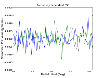
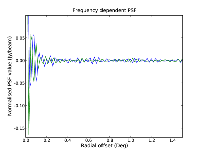
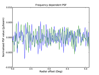
Figure 3.— Cuts through the Point Spread Function (PSF) for the 512-element array. Three different rows shows three different weighting schemes. Natural (Top Row), Robust 0.0 (Middle Row) and Uniform (Bottom Row). The left column zooms into the near side-lobe levels while the right column shows the far-away side-lobe levels. The abscissa shows the degree-offset from the center of the PSF. The two different curves in all the plots shows the PSF variation from two channels separated by 32 MHz in frequency.

We recognize that the choice of optimal weighting scheme depends on a number of parameters based on the array configurations, telescope hardware specifications and also on precise data reduction algorithms used. Hence all the upcoming EoR experiments need an optimal weighting scheme for their individual data reduction procedures. However, exploring the optimal weighting scheme is beyond the scope of this paper. For our work, we have adopted natural weighting scheme.

PSF side-lobe level reduces with increase in Hour Angle coverage. In our simulations we have used six hours of observing time to produce each data-set. However, in the actual experiment the observing time for each data-set may be less than that. Hence the PSF side-lobe level will also degrade accordingly.

4. Foreground Source Model - GSM

Our foreground sky model only includes point sources. No extended emission from galactic foreground is included as a part of the sky model. Recently, there has been extensive research regarding the foreground source removal dealing with sources below $S_{cut}=1$ Jy level. Most of these analysis implicitly assume that foreground sources above the $S_{cut}$ level are being removed perfectly. But in reality any imperfect calibration will introduce artifacts in the residual data after source removal. Hence in this paper our main aim is to explore the level of accuracy needed in these calibration procedures in order to ensure the residual errors from the strong foreground source removal do not obscure the detection of the signal from cosmic reionization. The choice of $S_{cut}$ level is not totally arbitrary and will be discussed in the final section of this paper.

The sky model is derived from the LogN-LogS distribution of sources and is termed as the Global Sky Model (GSM) from now onwards. Since our GSM only includes sources above 1 Jy, we follow the source count from the 6C survey at MHz (Hales et al. 1988). The source count from the 6C survey is given as:

$$N(>S_{Jy})=3600~{}S_{Jy}^{-2.5}Jy^{-1}str^{-1}$$ (5)

For a field-of-view of $15^{o}$ the total number of sources ($>1$ Jy) equates to $\sim 170$, following the above power-law distribution. The entire flux range between 1 - $10^{3}$ Jy was divided into several bins. The source population in each of these bins has been predicted following the above LogN-LogS distribution. In order to assign fluxes to individual sources inside a bin, a Gaussian random number generator has been used. The strongest source in our GSM is $\sim 200$ Jy. The center of the field is chosen such that it coincides with one of the cold spots in the foreground galactic emission seen from the southern hemisphere. Southern Sky is chosen since both the upcoming arrays MWA and PAPER are being constructed in Western Australia. The exact field center used for the GSM is 4 hours in Right Ascension and -26 degree in Declination. In order to assign a position to each of these sources within the field-of-view, another Gaussian random number generator has been used which predicted the offset from the field center for respective sources. In the GSM all the foreground sources are flat spectrum, i.e. with zero spectral index ($\alpha=0$).

Figure 4 shows the CLEANed image of the GSM used for all of the simulations. The CLEAN algorithm used in this process is a wide-field variant of the well-known Clark-CLEAN algorithm, which uses w-projection algorithm for 3-dimensional imaging.

In practice, the upcoming EoR telescopes should be using a similar Global Sky Model (GSM) but created from the existing source catalogs available for the part of the sky and frequency ranges of their observations. These telescopes will use the GSM as the preliminary sky model in order to detect and subsequently remove the bright foreground sources in the observed data-set.

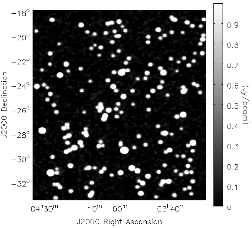
Figure 4.— Image of the Global Sky Model centered on RA=4h and DEC=$-26^{o}$. Clark-CLEAN has applied to this image using w-projection (256 planes) and Natural Weighting.

5. EoR Signal extraction - Data Reduction Procedure

All the simulations have been performed within the CASA package . As mentioned before, simulations for both 512-elements as well as 128-elements have been conducted and compared in the later sections.

The $15^{o}$ field-of-view will include $\sim 170$ bright sources ($>1$ Jy). The individual flux densities of these foregrounds are $\sim 10^{5}-10^{7}$ time higher than the signal from cosmic reionization that these instruments are aiming to detect. So the challenge lies in calibration and subsequent removal of such bright sources from the raw data-sets. In order to add to the constraints, the data rates of most of these telescopes (e.g. $\sim 19$ GB/s for MWA; Mitchell et al. (2008)) will not allow them to store the raw visibilities produced by the correlator. Hence real-time calibration and imaging needs to be done in order to reduce the data volume and store the final product in the form of image cubes (Mitchell et al. 2008). The critical steps include removal of the bright sources above the $S_{cut}$ level from the data-sets in these iterative rounds of real-time calibration and imaging procedure. As a result the residual image-cubes will not be dominated by these bright sources and the rest of the foregrounds can be removed in the image domain.

However, the accuracy of the foreground source removal strategies are strongly dependent on the data reduction procedure. The likely data reduction procedure which will be followed by the upcoming telescopes can be outlined as :

• The raw data-sets from the correlator will go through real-time calibration and subsequent removal of the bright sources based on some Global Sky Model (GSM), down to $S_{cut}$ level, in the UV domain.

• The residual data-sets will be imaged and stored as a cube for the future processing and removal of sources which are below $S_{cut}$.

However, due to imperfect calibration during the process of real-time calibration and source removal if any systematic error is incorporated in the residual image-cubes they cannot be minimized by simply averaging over a large number of such residual image-cubes. Hence to understand the level of accuracy required in the calibration procedure to reduce the residual systematic errors in the data-set is critical.

Here, we outline the reduction pathway that have been followed throughout the paper :

• The observed visibilities ($V_{ij}^{Obs}$ or $V_{ij}^{GSM_{perfect}}$) are simulated for 6 hours ($\pm 3$ hours in Hour-angle) from the GSM (with no position or flux error) and the array configuration from Table: 1.

• Model visibilities ($V_{ij}^{mod}$) are also generated using the same GSM but they are now corrupted with either GSM position errors or with residual calibration errors.

• Model visibilities are subtracted from the observed visibilities to residual visibilities ($V_{ij}^{res}=V_{ij}^{obs}-V_{ij}^{mod}$). This step will be referred to as UVSUB (Cornwell et al. 1992).

• We fit a third order polynomial in frequency to the dirty image-cube ($I^{res}$) formed from $V_{ij}^{res}$. This step will be referred to as IMLIN (Cornwell et al. 1992).

After the IMLIN step, we investigate the RMS noise in the residual image cube. We have tried to use different orders of polynomial for the IMLIN step but our conclusions did not change significantly. This may be mainly due to the fact that the only frequency dependent term in these simulations is the PSF. However, it should be mentioned in this context that on using higher order polynomials in the IMLIN step we will be taking out relevant structures at those scales in the frequency space (McQuinn et al. 2006). Since the reionization signal is a spectral signature with a width $\lesssim 2.5$ MHz (size of the largest possible CSS), using a very higher order polynomial in the IMLIN might remove the signature itself.

We have also explored UVLIN (Cornwell et al. 1992), which fits a polynomial in the UV domain to $V_{ij}^{res}$. But UVLIN works perfectly only within a small field-of-view depending on the channel width in frequency (Cornwell et al. 1992). Hence, in our proposed reduction pathway we are using UVSUB followed by IMLIN only.

6. Error Propagation

In this section we describe the effects of different errors arising from radio interferometric data processing and how they propagate and show up as artifacts in the final residual image. Here, we consider effects of the errors arising from the imperfect GSM and residual calibration errors on removal of strong foregrounds.

6.1. Error due to approximate GSM - Simulations

The source positions in the Global Sky Model (GSM) are accurate up to a level, e.g. the NVSS catalog has an accuracy of $\sim 6$ arc-seconds in positions of the sources detected (Condon et al. 2002). The real-time calibration procedure for MWA like telescopes might implement some method to iteratively solve for the positions of bright sources taking the initial value from the GSM, e.g. Asp-CLEAN (Bhatnagar & Cornwell 2004). An iterative scheme will also converge with some residual position and flux errors in the model. Hence, any error in the final GSM position or flux will contribute to imperfect source removal. The resultant artifact will limit the dynamic range in the residual data-set and obscure the detection of the faint signal from reionization. The main aim of the simulations in this section is to determine the accuracy of the GSM (position and flux) required in order to reach the required RMS noise level. The GSM position errors considered in the following simulations are actually systematic residual errors after the iterative position determination. Here, we deal with residual GSM errors in position and will also mention briefly the effect of the GSM flux errors in the residual data-set.

In order to introduce the position error in the GSM we have added an error term in the Right Ascension ($\alpha$) of each of the sources in the GSM. This error term is derived from a Gaussian distribution:-

$$\epsilon(\alpha)=\frac{1}{\sigma\sqrt{2\pi}}e^{\frac{\alpha^{2}}{2\sigma^{2}}}$$ (6)

where $\sigma$ denotes the error level in the position, i.e. for NVSS catalog $\sigma=6$ arc-seconds.

The steps in the simulation performed in order to explore the effect of the GSM error in position is as follows:

1. $V_{ij}^{Obs}$ are simulated.

2. Predict model visibilities from the GSM model with source-position error ($V_{ij}^{GSM_{imperfect}}$).

3. Subtract the model visibilities from the observed visibilities to get $V_{ij}^{Res}=V_{ij}^{GSM_{perfect}}-V_{ij}^{GSM_{imperfect}}=V_{ij}^{GSM_{error}}$.

4. Make $I^{res}$ and apply IMLIN as mentioned befor.e

In order to explain the above mentioned steps in detail we refer to figure 5, which demonstrates the procedure of the reduction followed in the simulations involving GSM errors. Figure 5a shows the dirty map (peak value: $\sim 2\times 10^{-3}$ Jy/beam) from the residual visibilities where the model visibilities where corrupted with a GSM position error of 0.01 arc-second. Figure 5b (peak value: $\sim 8\times 10^{-5}$ Jy/beam) is generated after applying IMLIN to the residual image. The gray-scale color-bars represent the variation of the intensity in two images.

6.2. Position Error in the GSM - Results

Here we discuss the implications of the results from the simulations with the GSM errors. Figure 6a represents the variation in the RMS noise level of three regions in : [1] True Image of $V_{ij}^{Obs}$ (figure 4), [2] Image of $V_{ij}^{Res}$ after UVSUB (figure 5a) and [3] Image after IMLIN (figure 5b). The GSM position errors used in this case is 0.01 arc-second.

In figure 6b, the RMS noise value in three different parts of the field-of-view have been plotted as a function of different residual GSM position errors. The RMS values quoted here are from the images of residual visibilities after UVSUB [2]. Hence the solid line denotes the trend in the decrease of the RMS noise in the UVSUB image with the decrease in the GSM position error. The magnitude of the position error (value of $\sigma$ as in equation 6) has been varied from 6 arc-seconds (as in NVSS catalog) down to an extremely low value of $10^{-4}$  arc-seconds. The original simulations were performed with 128-element array and the resulting RMS values are scaled down by factor of 5 in order to represent the same for the 512-element array. This scaling property has already been discussed in details in section-3 of this paper. According to the figure 6b it is evident that an accuracy of 0.1 arc-second in GSM position is needed to achieve the required RMS noise in order to detect the reionization signal after removal of strong foreground point sources. The solid curve in figure 6b represents the mean curve of the RMS noise level variation and has a mean slope of $\sim 1$ in the log-log space. This means that a decrease in the RMS noise level by another order of magnitude is possible on achieving an extra order of magnitude accuracy in the GSM position estimates.

Voronkov & Wieringa (2004) have shown similar results in demonstrating the effect of the pixelation error on the dynamic range of the image. Recently, Cotton & Uson (2008) have shown that a image made from a data-set using the VLA (27-element) obtains a dynamic range limitation of $10^{5}$ when the sources are shifted by 0.01 pixel in the image plane. This result is similar to the result quoted in figure 6b, where it is evident that GSM position error of 1 arc-second ($\sim 0.01$ pixel) results in an RMS noise of $\sim 10^{-4}$ Jy/beam corresponding to a dynamic range (DR) of $\sim 10^{6}$. The better PSF side-lobe level in 512-element array over VLA27-element array causes an extra order of magnitude gain in the dynamic range in the case of the former.

Here, we have considered only systematic residual GSM position errors which are the same from one day to the another. This will not reduce after averaging over residual image-cubes from successive days of observations. The real-time calibration system might implement an iterative scheme (e.g. Asp-CLEAN, Bhatnagar & Cornwell 2004) to determine the source positions. However, unless the systematic error determined by any such scheme is smaller than 0.1 arcsecond, averaging over long lengths of time will not mitigate the errors due to imperfect GSM. The GSM position error limit that we report in this paper is thus also applicable for the specifications of the accuracy that any such scheme delivers.

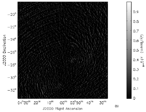
Figure 5.— (a)Dirty UVSUBed image of the field made from $V_{ij}^{res}$ after the imperfect GSM ($V_{ij}^{GSM_{imperfect}}$) has been subtracted from the perfect data-set ($V_{ij}^{obs}$). (b) The image of the field after the IMLIN has been applied to the UVSUBed image in figure a.

6.3. Flux Error in the GSM - Results

In this section we discuss the results of introducing GSM flux error in our simulations. GSM flux errors have been derived from a Gaussian random distribution (similar to equation 6) with mean zero and $\sigma\sim 0.1\%$ of flux values of respective sources. Similar to the steps of simulations discussed in section 6.1, the GSM model with flux error is used to corrupt model visibilities. The residual image cube shows sources with flux values of $\lesssim 0.1\%$ of the original sources in the same position. Since the GSM contains only sources between 1 Jy and $\sim 200$ Jy, the maximum residual flux density in the residual image is $\lesssim 0.2$ Jy/beam and can be denoted as sources below the $S_{cut}$ limit (Mitchell et al. 2008). The removal of such sources are beyond the scope of this paper.

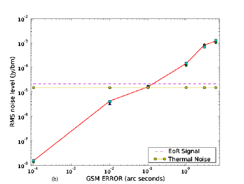
Figure 6.— (a) The RMS noise variation in three different parts of the images formed in the 3 steps of data reduction : [1] True Image (Figure 4) $\rightarrow$ [2] UVSUB image (Figure 5a) $\rightarrow$ [3] IMLIN image (Figure 5b). The GSM position error of 0.01 arc-seconds is used here. (b) The variation of RMS noise in the image plane with the GSM error in position. Both the figures also include the theoretical prediction for the EoR signal level ($22~{}\mu$ Jy/beam) and the thermal noise ($15.4~{}\mu$ Jy/beam) after $5\times 10^{3}$ hours of observations.

Flux errors might be as high as $\sim 1\%$, as quoted for most of the source catalogs such as NVSS. The residuals will show up as sources with flux density as high as few Jy/beam. In this case the residuals are well above the level of the $S_{cut}$ and perfect removal of such sources in the subsequent IMLIN step still remains a challenge.

6.4. Effect of Residual Calibration Errors - Simulations

This section deals with the effect of residual calibration error in the foreground source subtraction from the raw data-set coming out of the upcoming EoR instruments.

The antenna dependent complex gains can be defined as:

$$V_{ij}^{Corr}(t)=g_{i}(t)g_{j}^{*}(t)V_{ij}^{o}(t)$$ (7)

where $g_{i}$ ’s are the antenna dependent complex gains, $V_{ij}^{Corr}$ are the corrupted visibilities and $V_{ij}^{o}$ are the true visibilities or $V_{ij}^{GSM_{perfect}}$ in our case; $t$ denotes time variation.

The model for the complex gains used in the simulations is given by:

$$g_{i}(t)=(1+a_{i}+\delta a_{i}(t))exp(i(\phi_{i}+\delta\phi_{i}(t))$$ (8)

where $a_{i}$, $\phi_{i}$, $\delta a_{i}(t)$ and $\delta\phi_{i}(t)$ are for amplitudes ($a$) and phases ($p$). The gains in both amplitude and phase are derived from individual Gaussian random distribution as in equation 6.

The process of simulation is as follows :

1. $V_{ij}^{Obs}$ are simulated.

2. Model visibilities are predicted from a perfect GSM and are corrupted with $g_{i}(t)\&g_{j}(t)$ to compute $V_{ij}^{Corr}$

3. In UVSUB we get : $V_{ij}^{Res}=V_{ij}^{GSM_{perfect}}(g_{i}g_{j}^{*}-1)$.

4. Make $I^{Res}$ and apply IMLIN as mentioned before.

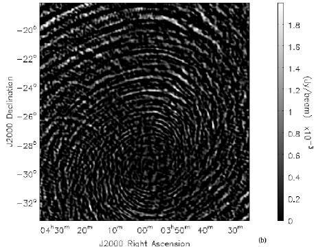
Figure 7.— (a) Dirty UVSUBed image of the field made from the $V_{ij}^{res}$, after the model visibilities corrupted with residual calibration errors ($V_{ij}^{Corr}$) has been subtracted from the perfect data-set ($V_{ij}^{Obs}$). (b) The image of the field after the IMLIN has been applied to the UVSUBed image in figure a.

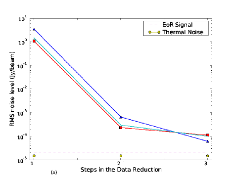
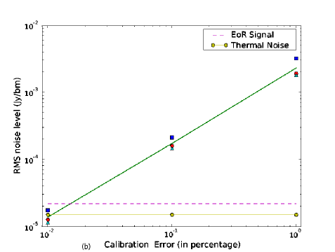
Figure 8.— (a) The RMS noise variation in three different parts of the images formed in the 3 steps of data reduction : [1] True Image (Figure 4) $\rightarrow$ [2] UVSUB image (Figure 7a) $\rightarrow$ [3] IMLIN image (Figure 7b). The calibration error used here is $0.1\%$ in amplitude or 0.1 degree in phase. (b) The variation of RMS noise in the image plane with the Residual Calibration error. The values denote the amplitude gain error in percentage or similar error in degree for the phase gain. Both the figures also include the theoretical prediction for the EoR signal level ($22~{}\mu$ Jy/beam) and the thermal noise ($15.4~{}\mu$ Jy/beam) after $5\times 10^{3}$ hours of observations.

The model for the complex antenna-dependent gain errors (equation 7) includes two terms for amplitude ($a_{i}$) and phase $\phi_{i}$ gains, which are constant for each antenna throughout each day of observing (6 hours). Along with them there are also two small additive random offsets $\delta a_{i}~{}\&~{}\delta\phi_{i}$, which vary within a single day of observation. Following Perley (1999), it has been determined through several simulations that the constant offsets ($a_{i},\phi_{i}$) are the dominant terms compared to the time dependent terms. Moreover, since the time variation for $\delta a_{i}~{}\&~{}\delta\phi_{i}$ are derived from a Gaussian distribution similar to equation 6, the effect of these terms decreases upon averaging over time. Hence, in our simulations we have only included the constant gain errors $a_{i}~{}\&~{}\phi_{i}$ and redefined equation 8 as :

$$g_{i}(t)\sim(1+a_{i})e^{i\phi_{i}}$$ (9)

It is certainly evident that some variant of the self calibration algorithm will be implemented in the real-time calibration procedure for the upcoming MWA like telescopes in order to facilitate the bright foreground source removal. In our simulations, we have not implemented any form of calibration algorithm. Instead, we have used the measurement equations with residual calibration errors in order to explore the accuracy with which any calibration procedure must work in order to achieve the desired RMS noise limit and detect the signal from reionization.

6.5. Effect of Residual Calibration Errors - Results

Figure 7 demonstrates the three steps followed to simulate the effect of the residual calibration errors in the EoR data-set. Figure 7a shows the dirty image of the residual UVSUB data and Figure 7b shows the image after IMLIN. Both these figures are from the simulation with $0.1\%$ amplitude error or $0.1$ degree phase error.

Figure 8a shows the variation in the RMS noise level in the three regions of the images made using : [1] $V_{ij}^{Obs}$ (figure 4), [2] $V_{ij}^{Res}$ in UVSUB (figure 7a) and [3] after IMLIN (figure 7b). It is clear from figure 8a that the RMS noise level reached near the bright sources after the UVSUB stage is $\sim 10^{-3}$ Jy/beam, corresponding to a dynamic range of $\sim 10^{5}$. Perley (1999) calculated the dynamic range limitation due to a time independent amplitude error in all the baselines that will be introduced to a point source data. If we denote the visibility function ($V_{ij}$) as :

$$V_{ij}(\vec{u})=(1+a)e^{i\phi}$$ (10)

where $a~{}\&~{}\phi$ are the amplitude and phase errors respectively, the dynamic range of the image is limited to :

$$DR\sim\frac{\sqrt{N(N-1)}}{\sqrt{2(a^{2}+\phi^{2})}}$$ (11)

where N is the number of antennas. In our case, $N=512$, $a=0.1\%$ and $\phi=0.1$ degree. These values yield a dynamic range of $\sim 10^{5}$, which agrees with the dynamic range we obtained from our simulations.

Figure 8b denotes the RMS noise value in different parts of the UVSUBed image as a function of different residual calibration errors. The three different residual calibration errors considered here are $0.01\%$, $0.1\%$ and $1\%$ in amplitude or 0.01 degree, 0.1 degree and 1 degree in phase respectively. The resultant curve in the log-scale has a slope of $\sim 1.1$. This indicates that in order to achieve the desired RMS noise level to detect the reionization signal, the residual calibration errors should be $\sim 0.01\%$ in amplitude or $\sim 0.01$ degree in phase. In practice, it is extremely challenging to achieve such accuracy with a real-time calibration procedure. Here, we have only considered systematic residual calibration errors which will not vary from one day to the other.

As before, these simulations were originally performed for the 128-element array and then the RMS noise values were scaled down by a factor $\sim 5$ following the scaling property that has been discussed in initial sections. However, we have also repeated the simulations for the 512-element array with residual calibration error of $0.1\%$ in amplitude or 0.1 degree in phase and found the results consistent with our scaled values.

6.6. Reducing the effect of the residual calibration error

In the previous section it is clearly shown that even the low systematic residual calibration errors restrict the dynamic range in the residual image to $10^{5}$, whereas the desired dynamic range is $\sim 10^{8}$ in order to detect the signal from reionization.

The obvious next step to follow is to add the UVSUBed image cubes from successive days in order to check whether the residual calibration error reduces as $\propto 1/\sqrt{N_{days}}$, where $N_{days}$ denotes the number of days over which the UVSUB images has been added and each day consists of 6 hours of observations. We can demonstrate the same from the expression of the residual visibilities ($V_{ij}^{Res}=V_{ij}^{GSM_{perfect}}(g_{i}g_{j}^{*}-1)$). If the calibration procedure is able to remove all systematic gain errors from the corrupted data contributing to residual calibration errors that are purely random from day to day, then they will reduce upon averaging.

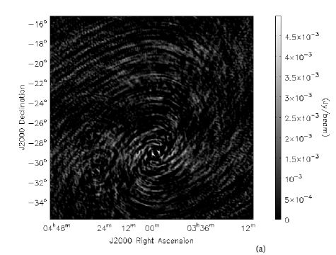
Figure 9.— (a) Dirty UVSUBed image of the field made from the $V_{ij}^{res}$, after the model visibilities corrupted with residual calibration errors ($V_{ij}^{Corr}$) has been subtracted from the perfect data-set ($V_{ij}^{Obs}$). (b) The averaged dirty image of the field after averaging 20 days of individual UVSUBed image, such as in figure a.

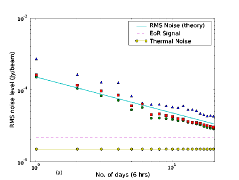
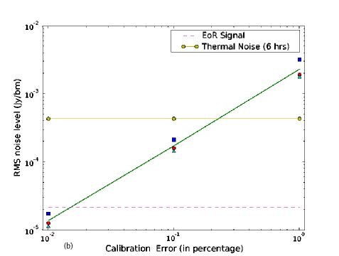
Figure 10.— (a) The RMS noise variation in three different part of the field shown as a function of the days of integration. The solid line denotes the theoretical curve, showing a $\propto 1/\sqrt{N_{days}}$ dependence of the RMS noise reduction. The figure also includes the theoretical prediction for the EoR signal level ($22~{}\mu$ Jy/beam) and the thermal noise ($15.4~{}\mu$ Jy/beam) after $5\times 10^{3}$ hours of observations. (b) The variation of RMS noise in the image plane with the Residual Calibration error. The values denote the percentage error in the amplitude gain and similar error in degree for the phase gain. The thermal noise quoted here is $433~{}\mu$ Jy from 6 hours of integration (1 day).

Figure 9 demonstrates the effect of the averaging over 20 days of UVSUBed images with the residual calibration errors of $0.1\%$ in amplitude or $0.1$ degree in phase. Figure 9a denotes the dirty image after the first day and figure 9b denotes the averaged image after 20 days. The figures demonstrate a significant reduction in the RMS noise level after 20 days of averaging. Figure 10a shows the reduction in the RMS noise level in different parts of the image on averaging over $20$ days. The solid line denotes the theoretical noise curve that follows $\propto 1/\sqrt{N_{days}}$. Hence, the reduction in RMS noise on averaging over different days is consistent with the theoretical prediction ($\propto 1/\sqrt{N_{days}}$).

A UVSUBed image from each day (6 hours) is also limited by the thermal noise, which reduces down as $\propto 1/\sqrt{N_{days}}$. If the residual calibration errors are random between successive data-sets from different days of integration then it should also reduce down as $\propto 1/\sqrt{N_{days}}$. As a result, it should then be sufficient to achieve a resultant RMS noise level in the images below the daily thermal noise limit. From Table 1 we can estimate that the thermal noise limit from 1 day of integration (6 hours) is $\sim 433~{}\mu$ Jy/beam. Figure 9b is the same as figure 8b except that we have plotted the new noise estimates from 6 hours of observation. This figure now explains that the residual calibration errors should be $\sim 0.2\%$ in amplitude or $\sim 0.2$ degree in phase in order to reach below the daily thermal noise limit. Once the RMS noise level in the UVSUBed image is below the daily thermal noise limit, it can reduce down along with the thermal noise in order to detect the faint reionization signal within the time limit set by the telescope sensitivity (i.e. $5\times 10^{3}$ hours).

The most important caveat in the entire analysis is the fact that we assume that the residual calibration errors are not systematic from one day to the next. If there are any systematics left over from day to day (e.g. due to antenna gain errors, antenna primary beam errors, pointing errors, etc) then those will not go down as $\propto 1/\sqrt{N_{days}}$. Moreover, even with these assumptions the much needed accuracy in calibration is alarmingly high.

7. Discussion - Implications on the upcoming arrays

There are few important results and concerns that have come out from the simulations performed in this paper.

The simulations have been performed for both 128-element array and 512-element array. Necessary comparisons between both arrays have been discussed at essential stages of this paper. The comparison between the two configuration can be well explained by a simple scaling relation which is the ratio between the RMS value of the PSF side-lobe levels in two configurations. Hence it was sufficient to perform the 512-element simulations only for the optimal value of the GSM position error and residual calibration error.

The choice of $S_{cut}=1$ Jy in our GSM is not totally arbitrary keeping in mind the fact that the real-time calibration procedure needs to model and remove all the sources down to $S_{cut}$ from the raw UV data-sets within a duration constrained by the instrumental specifications. Since the errors we have discussed in this paper are dominated by the bright sources inside the field-of-view, our analysis will not change significantly by reducing the $S_{cut}$ level and including more and more fainter sources.

Our simulations show two major results about the accuracy required to reach the desired RMS noise level in order to detect the reionization signal :

• GSM position accuracy of $\sim 0.1$ arc-second

• Tolerance of residual calibration errors of $\lesssim 0.2\%$ in amplitude or $\lesssim 0.2$ degree in phase.

In the section dealing with the GSM position errors, we have only discussed about systematic errors which do not change from one day to the next. If the calibration procedure involves some iterative position calibration scheme that will evaluate the source position everyday then the errors from those procedure should vary from one day to the other. Hence, there is a possibility of reaching the desired RMS noise level even with lesser accuracy in the GSM position estimates.

In practice, a better GSM can be obtained a priori from a deep survey of the specific fields to be observed with MWA, LOFAR, etc. using the present facilities like GMRT and WSRT (Bernardi et al. 2009) at 150 MHz. MWA, LOFAR, etc can also improve the existing GSM after sufficient days of observations.

The simulations with calibration errors assume that the image cubes are formed after each day of observations (6 hours). We assume that the calibration errors are incoherent beyond 6 hours and as a result the effect of calibration error will reduce with successive days of integration. If calibration error have shorter coherence time, then lesser accuracy in the calibration can be tolerated in order to reach below the thermal noise limit for the shorter integrations. However, the systematics need to be removed at those timescales to make sure that the residual errors are still random from one data-set to the next. It should be noted that the PSF side-lobe level will also be higher due to shorter integration period, which in turn might make it harder to solve and remove the systematics at a shorter timescales.

The data analysis pipeline adapted in this paper resembles mostly the upcoming MWA telescope. Since the raw visibilities cannot be stored, the calibration and removal of the brightest sources in the real-time calibration pipeline is one of the major step in foreground subtraction (Mitchell et al. 2008). The accuracy in GSM position and residual calibration (discussed in this paper) is critical for extraction of the EoR signal. In other telescopes like LOFAR, where it is possible to store the raw visibilities, the calibration will be carried out through a combination of real-time processing and off-line reprocessing scheme. The ability to store the raw visibilities will allow more accurate calibration of the data in the off-line mode. However, the combination of real-time and off-line calibration pipeline for LOFAR still needs to achieve similar accuracy in calibration (discussed in this paper) in order to reach the desired dynamic range to extract the EoR signal.

In the present paper we have not discussed in great detail the step of polynomial fitting in the image domain. This is mainly because the lack of frequency dependence of the sky model as well as the instrumental gain model. Our simulations do not include thermal noise. In practice, the IMLIN step should be applied to the residual image-cubes, averaged over total number of days required to beat thermal noise. Hence, it should produce similar decrease in the RMS noise level as obtained in this paper on “noise-less” data.

The major feedback from all these simulations that we get is that the raw UV-data should be retained, even considering the huge data-rate issue, until the iterative real-time calibration procedures achieve the desired accuracy. Upcoming telescopes like MWA, PAPER, LOFAR, etc will also be trying to detect the EoR signal in the Power Spectral domain. Hence, a relevant extension of our present work will be to extend these analysis into the power spectral domain. We are also planning to deal with frequency dependent and direction dependent calibration errors in subsequent publications.

References

- Backer et al. (2007) Backer, D. C., Parsons, A., Bradley, R., Parashare, C., Gugliucci, N., Mastrantonio, E., Herne, D., Lynch, M., Wright, M., Werhimer, D., Carilli, C., Datta, A., & Aguirre, J. 2007, in Bulletin of the American Astronomical Society, Vol. 38, Bulletin of the American Astronomical Society, 967–+
- Bernardi et al. (2009) Bernardi, G., de Bruyn, A. G., Brentjens, M. A., Ciardi, B., Harker, G., Jelić, V., Koopmans, L. V. E., Labropoulos, P., Offringa, A., Pandey, V. N., Schaye, J., Thomas, R. M., Yatawatta, S., & Zaroubi, S. 2009, A&A, 500, 965
- Bhatnagar & Cornwell (2004) Bhatnagar, S. & Cornwell, T. J. 2004, A&A, 426, 747
- Bowman et al. (2008) Bowman, J. D., Morales, M. F., & Hewitt, J. N. 2008, ArXiv e-prints
- Briggs et al. (1999) Briggs, D. S., Schwab, F. R., & Sramek, R. A. 1999, in Astronomical Society of the Pacific Conference Series, Vol. 180, Synthesis Imaging in Radio Astronomy II, ed. G. B. Taylor, C. L. Carilli, & R. A. Perley, 127–+
- Carilli et al. (2002) Carilli, C. L., Gnedin, N. Y., & Owen, F. 2002, ApJ, 577, 22
- Condon et al. (2002) Condon, J. J., Cotton, W. D., Greisen, E. W., Yin, Q. F., Perley, R. A., Taylor, G. B., & Broderick, J. J. 2002, VizieR Online Data Catalog, 8065
- Cornwell et al. (1992) Cornwell, T. J., Uson, J. M., & Haddad, N. 1992, A&A, 258, 583
- Cotton & Uson (2008) Cotton, W. D. & Uson, J. M. 2008, A&A, 490, 455
- Di Matteo et al. (2002) Di Matteo, T., Perna, R., Abel, T., & Rees, M. J. 2002, ApJ, 564, 576
- Fan et al. (2006a) Fan, X., Carilli, C. L., & Keating, B. 2006a, ARA&A, 44, 415
- Fan et al. (2006b) Fan, X., Strauss, M. A., Becker, R. H., White, R. L., Gunn, J. E., Knapp, G. R., Richards, G. T., Schneider, D. P., Brinkmann, J., & Fukugita, M. 2006b, AJ, 132, 117
- Furlanetto et al. (2006) Furlanetto, S. R., Oh, S. P., & Briggs, F. H. 2006, Phys. Rep., 433, 181
- Gleser et al. (2008) Gleser, L., Nusser, A., & Benson, A. J. 2008, MNRAS, 391, 383
- Hales et al. (1988) Hales, S. E. G., Baldwin, J. E., & Warner, P. J. 1988, MNRAS, 234, 919
- Harker et al. (2009) Harker, G., Zaroubi, S., Bernardi, G., Brentjens, M. A., de Bruyn, A. G., Ciardi, B., Jelić, V., Koopmans, L. V. E., Labropoulos, P., Mellema, G., Offringa, A., Pandey, V. N., Schaye, J., Thomas, R. M., & Yatawatta, S. 2009, MNRAS
- Jelić et al. (2008) Jelić, V., Zaroubi, S., Labropoulos, P., Thomas, R. M., Bernardi, G., Brentjens, M. A., de Bruyn, A. G., Ciardi, B., Harker, G., Koopmans, L. V. E., Pandey, V. N., Schaye, J., & Yatawatta, S. 2008, MNRAS, 389, 1319
- Komatsu et al. (2008) Komatsu, E., Dunkley, J., Nolta, M. R., Bennett, C. L., Gold, B., Hinshaw, G., Jarosik, N., Larson, D., Limon, M., Page, L., Spergel, D. N., Halpern, M., Hill, R. S., Kogut, A., Meyer, S. S., Tucker, G. S., Weiland, J. L., Wollack, E., & Wright, E. L. 2008, ArXiv e-prints
- Labropoulos et al. (2009) Labropoulos, P., Koopmans, L. V. E., Jelic, V., Yatawatta, S., Thomas, R. M., Bernardi, G., Brentjens, M., de Bruyn, G., Ciardi, B., Harker, G., Offringa, A., Pandey, V. N., Schaye, J., & Zaroubi, S. 2009, ArXiv e-prints
- Liu et al. (2008) Liu, A., Tegmark, M., & Zaldarriaga, M. 2008, ArXiv e-prints
- Lonsdale et al. (2009) Lonsdale, C. J., Cappallo, R. J., Morales, M. F., Briggs, F. H., Benkevitch, L., Bowman, J. D., Bunton, J. D., Burns, S., Corey, B. E., deSouza, L., Doeleman, S. S., Derome, M., Deshpande, A., Gopalakrishna, M. R., Greenhill, L. J., Herne, D., Hewitt, J. N., Kamini, P. A., Kasper, J. C., Kincaid, B. B., Kocz, J., Kowald, E., Kratzenberg, E., Kumar, D., Lynch, M. J., Madhavi, S., Matejek, M., Mitchell, D., Morgan, E., Oberoi, D., Ord, S., Pathikulangara, J., Prabu, T., Rogers, A. E. E., Roshi, A., Salah, J. E., Sault, R. J., Udaya Shankar, N., Srivani, K. S., Stevens, J., Tingay, S., Vaccarella, A., Waterson, M., Wayth, R. B., Webster, R. L., Whitney, A. R., Williams, A., & Williams, C. 2009, ArXiv e-prints
- McQuinn et al. (2006) McQuinn, M., Zahn, O., Zaldarriaga, M., Hernquist, L., & Furlanetto, S. R. 2006, ApJ, 653, 815
- Mitchell et al. (2008) Mitchell, D. A., Greenhill, L. J., Wayth, R. B., Sault, R. J., Lonsdale, C. J., Cappallo, R. J., Morales, M. F., & Ord, S. M. 2008, ArXiv e-prints
- Morales et al. (2006a) Morales, M. F., Bowman, J. D., Cappallo, R., Hewitt, J. N., & Lonsdale, C. J. 2006a, New Astronomy Review, 50, 173
- Morales et al. (2006b) Morales, M. F., Bowman, J. D., & Hewitt, J. N. 2006b, ApJ, 648, 767
- Perley (1999) Perley, R. A. 1999, in Astronomical Society of the Pacific Conference Series, Vol. 180, Synthesis Imaging in Radio Astronomy II, ed. G. B. Taylor, C. L. Carilli, & R. A. Perley, 275–+
- Thomas et al. (2008) Thomas, R. M., Zaroubi, S., Ciardi, B., Pawlik, A. H., Labropoulos, P., Jelic, V., Bernardi, G., Brentjens, M. A., de Bruyn, A. G., Harker, G. J. A., Koopmans, L. V. E., Mellema, G., Pandey, V. N., Schaye, J., & Yatawatta, S. 2008, ArXiv e-prints