Generating and Analyzing Constrained Dark Energy Equations of State and Systematics Functions

Abstract

Some functions entering cosmological analysis, such as the dark energy equation of state or systematic uncertainties, are unknown functions of redshift. To include them without assuming a particular form we derive an efficient method for generating realizations of all possible functions subject to certain bounds or physical conditions, e.g. $w\in[-1,+1]$ as for quintessence. The method is optimal in the sense that it is both pure and complete in filling the allowed space of principal components. The technique is applied to propagation of systematic uncertainties in supernova population drift and dust corrections and calibration through to cosmology parameter estimation and bias in the magnitude-redshift Hubble diagram. We identify specific ranges of redshift and wavelength bands where the greatest improvements in supernova systematics due to population evolution and dust correction can be achieved.

I Introduction

The nature of the dark energy accelerating the cosmic expansion is a major mystery of modern physics. The effectively negative pressure giving rise to acceleration can be parametrized through the equation of state, or pressure to energy density, ratio of the dark energy. Observational quantities such as the distance-redshift relation, Hubble expansion rate, or matter density perturbation growth (assuming general relativity) can then be derived in terms of the equation of state (EOS). However, little guidance exists from theory for the form of the EOS.

One of the standard approaches is to adopt a well-tested, nearly unbiased functional form for the EOS. For example, the EOS as a function of scale factor, $w(a)=w_{0}+w_{a}(1-a)$, where $w_{0}$, $w_{a}$ are parameters to be fit, has been shown to be accurate at the $0.1\%$ level in the observable distance for a wide array of dark energy models calib . However, one may prefer to keep the EOS as free as possible. Values in bins of redshift, or some form of eigenmodes or principal components, do not impose assumptions on the form of $w(a)$ (see, e.g., hutstar ; coohut ; tobin ; mhh ; kitching ; mort09 ).

Physics does bound the possible behaviors, though, not allowing full freedom in the bin values or principal component coefficients. One example involves a minimally coupled, canonical scalar field, where for all redshifts the condition must hold that $w\in[-1,+1]$ for positive energy density. Principal components can be applied to many situations, such as the cosmic reionization fraction history or the fraction of a source population in a particular subclass, where values can only lie in $[0,1]$. We generically call such unknown, redshift dependent quantities “state functions”. Some approaches to such situations of “freedom under constraint” exist in the cosmology literature, e.g. mort1 ; tobin ; mhh ; lin0812 ; amara , but here we concentrate on full and computationally efficient solutions.

Going further into the motivation, we consider three reasons for imposing bounds: physicality, efficiency, and prior information. Some physical bounds are absolute, such as an ionization fraction ranging between 0 and 1, while others are more relative, such as the dark energy equation of state ranging between $-1$ and $+1$ for a canonical, minimally coupled scalar field. In fact, there is a certain amount of framework dependence in any analysis – the matter density cannot be less than zero, but the effective matter density can appear less than zero when a universe with a cosmological constant is interpreted in terms of a pure matter universe: this is precisely how the acceleration of the universe was discovered. So while physical bounds are generally valid, results pushing up against the bounds should sound a note of caution; one might then loosen the bounds to check for consistent results. But starting with overly loose or unmotivated bounds has the price of computational inefficiency; in the vast majority of cases one would not scan over a space where the ionization fraction ranged from $-5$ to $+5$, say. Finally, the bounds may arise from prior information such as having measured a calibration offset to be less than some value (as we apply in Sec. V). There is little point in examining the effect of larger variations than allowed by this prior information. These rationales for bounds on the state function then translate directly into the principal component space. We emphasize that only the amplitude, not the freedom in the functional form, is being limited.

When selecting physically valid principal component contributions the two main issues are those of purity – every set of values gives a valid state function – and completeness – every possible valid state function is represented in the selection. In Sec. II we discuss possible methods for generating principal component realizations of the EOS (or any other) function and assess their purity and completeness, especially when only a subset of modes is retained. We present a solution for the optimal – pure and complete – prescription in Sec. III, along with an efficient mathematical shortcut and visualization for implementing it. We then turn to state functions representing systematic uncertainties, whose evolution can cause incorrect cosmological conclusions. In Sec. IV we consider supernova population fractions as the constrained state function and investigate the biases this can impose on cosmological parameters, and how to best constrain these with redshift specific observations. We discuss dust extinction corrections and their interaction with filter calibration errors in Sec. V, and how to control these with wavelength specific measurements. The summary is presented in Sec. VI.

II Realizations of the Equation of State

We begin by phrasing the analysis in terms of the dark energy equation of state, although the results are generally applicable to any state function.

One possible goal for propagating an array of equation of state functions to observational constraints is to place as little prior constraint on the functions as possible, an admission of maximal ignorance in the hope that the observations impose form on chaos. A more restrained approach is to treat the form of deviations from the basic function as free, perhaps representing unknown systematic uncertainties, though bounded in amplitude in some way. The most direct approach then is to describe the deviations $w(z)-w_{b}(z)$ by some value in each small redshift bin, equivalent to expanding in a top hat basis.

This can be transformed into any other orthogonal basis and we can hope that a principal component analysis lets us compress the information in some way, such that a small, tractable number of modes gives a simplified, though still somewhat diverse, functional form. We can write

$$w(z)-w_{b}(z)=\sum_{i}\alpha_{i}\,e_{i}(z)\,,$$ (1)

where we refer to $w(z)-w_{b}(z)$ as the state function, $e_{i}(z)$ as the modes or principal components, and $\alpha_{i}$ as the mode coefficients. Note that the state function is really the deviation from some baseline, and can represent the dark energy equation of state or the cosmic ionization fraction, supernova subclass population fraction, etc. In the top hat basis, $e_{i}(z)$ would simply be 1 within the appropriate redshift bin and 0 outside, and $\alpha_{i}$ would simply be $w_{i}$, the value of the state function within the bin.

The state function may not be allowed to have arbitrary excursions, but can be constrained by physical or theoretical expectations to lie within some bounds. These bounds could be elementary, such as the ionization fraction must lie between 0 and 1, or more physical, such as the equation of state for a minimally coupled, canonical scalar field must possess $w(z)\in[-1,+1]$. We define the bounding function, or envelope, by

$$W_{-}(z)\leq w(z)-w_{b}(z)\leq W_{+}(z)\,.$$ (2)

Given real data, the results should localize within the bounds. One might be tempted to loosen the bounds and allow the data to lead to the proper area of parameter space. However, the data does not always have the required leverage to make this a successful approach. For example, if the equation of state rapidly oscillated between $-10$ and $+10$, this could not be detected in the distance measurements (or such an oscillation in ionization fraction, even to unphysical negative values, might not be seen in cosmic microwave background polarization measurements) but one has spent a lot of effort calculating over an enlarged range. Furthermore, when dealing with systematics, unknown by definition, or projected future measurements, if one does not bound the amplitudes then no real information can be obtained from the results. Thus, one has to balance reasonable, physical bounds and the computational efficiency with the desire not to restrict the input. We take $W_{-}$, $W_{+}$ to be defined with this in mind. The effects on the principal components of increasing the envelope are simply given by scaling $W_{-}$, $W_{+}$ in the formulas derived.

The question then becomes how to best incorporate these bounds in “configuration” (e.g. redshift) space into the coefficients of the principal components (PC) in mode space. For example, to generate realizations of state functions that are viable according to the bounds imposed, we must know how to properly sample the PC coefficients.

Several methods can be attempted, but must be assessed for their (computational) efficiency, purity, and completeness. The obvious, and least efficient method is simply to try values of the coefficients $\{\alpha_{1},\dots,\alpha_{N}\}$ and see if the functions $w(z)$ obey the bounds at each redshift. In practice one must truncate the number of PCs at a finite number, choose a finite range for each $\alpha_{i}$, and with a number of grid points $R$ sampling the coefficient range evaluate $R^{N}$ functions to test whether they lie within the bounds. For a grid of 20 points and 10 PCs, this requires $20^{10}\approx 10^{13}$ evaluations. We call this the scanning strategy. It would be pure and complete, but is not efficient.

A second approach is to ask that each PC contribution to the state function obey the bounds individually. This mode-by-mode strategy has been implemented in mort1 ; tobin ; mhh for example. Projecting a given PC against the state function yields the coefficient:

$$\alpha_{i}={\mathcal{N}}\int dz\,e_{i}(z)\,[w(z)-w_{b}(z)]\,,$$ (3)

where ${\mathcal{N}}=1/\int dz\,e_{i}^{2}(z)$ is the normalization factor. Incorporating the bounds on the state function and breaking the integration region into those redshifts where $e_{i}(z)$ is positive and those where it is negative, one obtains the bounds

$$\alpha_{i}^{-}\leq\alpha_{i}\leq\alpha_{i}^{+}\,,$$ (4)

where

$$\alpha_{i}^{\pm}=({\mathcal{N}}/2)\int dz \,\,\bigl{\{}\,\, [W_{+}(z)+W_{-}(z)]\,e_{i}(z)$$ (5)

$$\pm [W_{+}(z)-W_{-}(z)]\,|e_{i}(z)|\bigr{\}}\,.$$

The main problem with this approach is that the modes are treated independently. So if one saturates the bounds on each coefficient, say, then the generated state function may actually lie outside the envelope. Thus, this method is complete but not pure.

One way to incorporate all the mode information is to consider the integral of the square of the state function mhh . Then

$$\int dz\,[w(z)-w_{b}(z)]^{2}={\mathcal{N}}\sum_{i}\alpha_{i}^{2}\,.$$ (6)

Imposing the bounds on the state function then delivers the constraint

$$\sum_{i}\alpha_{i}^{2}\leq(1/{\mathcal{N}})\int dz\,{\rm max}\{W_{+}^{2}(z),W_{-}^{2}(z)\}\,,$$ (7)

where the maximum is to be evaluated for each redshift. (This generalizes the expression in mhh to when the envelope is not redshift independent.) We call this the integrated method and it defines a sphere in the mode coefficient space. This approach guarantees completeness but not purity, i.e. every viable state function can be generated with this set of coefficients, but nonviable ones can be as well. By itself it lacks a specific prescription for implementing the selection of $\alpha_{i}$’s.

An alternate approach is the “global” method, where coefficients are chosen based on the previous coefficient values. For example, choose the coefficient $\alpha_{1}$ based on the envelope constraint as if this were the only mode, giving

$$\frac{W_{\mp}(z)}{e_{1}(z)}\leq\alpha_{1}\leq\frac{W_{\pm}(z)}{e_{1}(z)}\,,$$ (8)

where the top (bottom) sign holds for $e_{1}(z)>0$ ($<0$). This is applied for all redshifts under consideration and the tightest constraints obtained define the range of $\alpha_{1}$. Once an $\alpha_{1}$ is sampled within the allowed range, one obtains similar bounds on $\alpha_{2}$ using, e.g., $\alpha_{2}\,e_{2}(z)\leq W_{+}(z)-\alpha_{1}\,e_{1}(z)$, and so on. This global method is simpler, not involving any integrals, although it still involves scanning over choices for the coefficients within their allowed range. However, a value for the coefficient $\alpha_{i}$ that has been rejected because it lies outside the bounds of Eq. (8) or similar may actually be valid because another PC counteracts its contribution and pulls the state function back within the envelope. Thus the method is pure, i.e. all generated state functions will be viable, but not complete.

Thus we have generating methods that are pure and complete but inefficient (scanning method), complete (mode-by-mode method), and pure (global method), but no obviously optimal method. We address this lack in the next section, and show how all the methods are related.

III A Pure and Complete Prescription

The physical bounds on the state function are imposed in the redshift space but we need to translate these into PC coefficient space if we want to generate principal component analysis (PCA) realizations of the state function. The problem is that a principal component contributes to the state function over the whole redshift interval considered. Effectively, PCA mixes the values $w_{i}$ from all redshift bins in the bin basis. Therefore what the chosen bound corresponds to – a value for the state function at a particular redshift $z$ – is not localized in coefficient parameter space but is described by a linear combination of many modes weighted by their respective coefficients.

III.1 Hypersurface Picture

However, by making use of the properties of linear transformations, and a particularly clear geometric picture, we can implement an exact, fast method for the translation. Consider the envelope on a single $w_{i}$. This gives a range, or line segment, along the $w_{i}$ axis. Combining the envelopes for all redshift bins, i.e. $w_{i}$ parameters, defines a hypersurface in an $N$ dimensional space, where $N$ is the number of redshift bins. If the bin bounds do not depend on values $w_{i}$ in other bins, i.e. each bin is independent (recall the original motivation was to consider state function behaviors without assuming a functional form), then the surface is a hyperrectangle.

The corners of the hyperrectangle are defined by the values $W_{\pm}(z_{i})$ of the envelope. These $2^{N}$ vertices contain all information on the boundary between the permitted, i.e. viable, instances of state functions $w(z)-w_{b}(z)$ and the disallowed or unviable ones. That is, the boundary defines the pure and complete set.

We defined the vertices as sets of $w_{i}$ coordinates but now let us consider the hypersurface in the PC coefficient space of $\alpha_{i}$ coordinates. Because the PCA is a (normalized) linear transformation of the redshift bin values, the hypersurface is merely rotated, not distorted or expanded. If we are interested in a subset of $M$ modes, smaller than the maximum number $N$ (there cannot be more modes than the original bins used to define the PCs), then this corresponds simply to a projection of the hypersurface onto the subspace of the $M$ PC coefficients. We illustrate the case of a 3 dimensional hyperrectangle projected onto 2 PC coefficients in Figure 1.

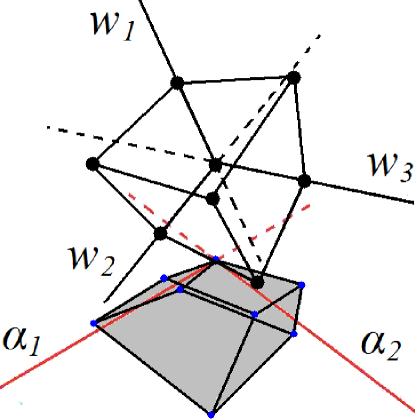
Figure 1: A cube in bin space, corresponding to redshift independent limits on $w(z)-w_{b}(z)$ in 3 redshift bins (i.e. the simplest nontrivial case of an $N$-dimensional hyperrectangle), is projected onto the parameter space of the coefficients of the first two principal components. The small blue dots indicate the projection of the cube vertices. The permitted area in the $\alpha_{1}$-$\alpha_{2}$ plane is indicated by the light grey shading. Note that it does not form a rectangle.

The boundary of the pure and complete set of PC coefficients is defined by connecting the outermost projected vertices ensuring the boundary remains convex. This follows from the linearity of the transform: the hypersurface is convex and so the projection must then itself be convex. (Note the projected figure is not in general rectangular.) The projection can be computed quite quickly through the use of matrix algebra (see the Appendix). Thus a pure and complete set of PC coefficients for viable, and only viable, state functions can be generated efficiently.

If we do a complete projection over all $N$ dimensions except one, say $\alpha_{j}$, we obtain the absolute minimum and maximum bounds on $\alpha_{j}$. These bounds are equivalent to those found with the mode-by-mode method, Eq. (4). Furthermore, since distances are conserved under the linear transformation, the maximum distance in bin space, i.e. the longest diagonal of the hyperrectangle, must also be the maximum distance in PC coefficient space. A (hyper)sphere with this diameter circumscribes the allowed set and corresponds to the sphere of the integrated method, Eq. (7). From the fact that the hypersphere circumscribes the hyperrectangle, it is clear that this method generates a complete, but not pure, set.

The degree of impurity or incompleteness for the methods can be tied to the ratios of areas (or hypervolumes) between the geometric figure defined by the methods and the true hyperrectangle. If the PC coefficients are highly independent of each other (of course the mode vectors $e_{i}$ themselves are orthogonal), then we expect the mode-by-mode method, where we ignored the effect of $\alpha_{j}$ on $\alpha_{i}$, to be a good approximation, i.e. nearly pure and complete. Taking zero correlation between coefficients defines a rectangle in the $\alpha_{i}$-$\alpha_{j}$ plane, for any $\alpha_{i}$, $\alpha_{j}$. As the coefficient parameters become more correlated, the mode-by-mode method should become less efficient at finding only the viable state functions, i.e. less pure. Geometrically, the filling factor of the true hyperrectangle projection will decrease.

Figure 2 illustrates this relation between correlation and filling factor. The top panel shows the projection onto the space spanned by the coefficients of PC modes 1 and 17. Since $e_{1}$ and $e_{17}$ have their main weights at very different redshifts, the coefficients $\alpha_{1}$ and $\alpha_{17}$ are substantially uncorrelated, and indeed the filling factor is high (but not perfect). The bottom panel displays the equivalent projection for modes 1 and 2. Here the overlap of the modes in redshift is greater and so the coefficients are more correlated; the filling factor is noticeably decreased. Therefore the mode-by-mode method is not efficient when considering the dominant modes.

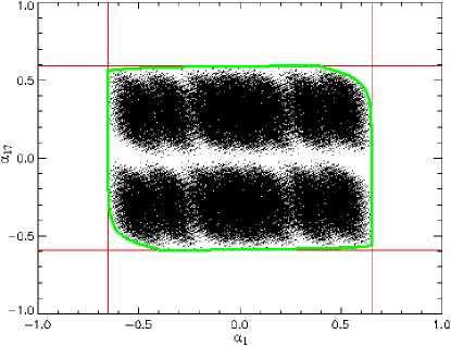
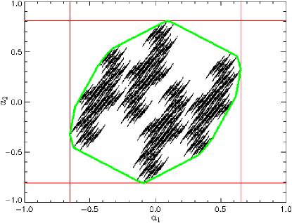
Figure 2: Projections onto PCA coefficient planes are shown for the 17 mode case. The light, red vertical and horizontal lines indicate the mode-by-mode bounds of Eq. (4). The dots give the projection of the $2^{17}$ vertices of the hyperrectangle, and the thick, green polygon gives the outer boundary, defining the interior region of pure and complete viable state functions. [Top panel] The $\alpha_{1}$-$\alpha_{17}$ plane in parameter space has low correlation between these modes, so the filling factor of the approximate bounds is high. [Bottom panel] The $\alpha_{1}$-$\alpha_{2}$ plane has strong correlations because the PCs overlap substantially in redshift, so the filling factor is low.

By contrast, the exact hyperrectangle projection method is highly efficient. For 10 modes, say, there are $2^{10}\approx 10^{3}$ vertices to evaluate (the projection takes negligible computational time using the method in the Appendix). Contrast this with the previous $10^{13}$ evaluations needed for direct scanning.

If we were to increase the number of redshift bins (i.e. bin modes, holding the redshift range constant), this allows for more and more PC modes. However, since most of these additional modes would be less and less correlated with a given mode, we effectively have a convergence in the behavior of the parameters, i.e. the projected boundary in a given $\alpha_{i}$-$\alpha_{j}$ plane.

In summary, we have presented an efficient, pure, and complete method of obtaining the boundary defining the set of viable state functions. The relation to previous (not simultaneously pure and complete) methods is illustrated in Figs. 3-4. The outer rectangle gives the prescription of the mode-by-mode approach; the thick interior polygon shows the exact solution using the projection of the hyperrectangle; and the light shaded interior non-rectangle illustrates the global method, representing a cut through the hyperrectangle at $\alpha_{i>2}=0$. Since the exact solution can be generated efficiently there is no need to use the over- (global) or under- (mode-by-mode) approximation.

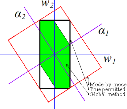
Figure 3: Three different approaches to obtaining the principal component coefficients for a constrained state function are illustrated, here for the first and second coefficients and the simplest case with only 2 modes. The true viable region is the thick black rectangle in $w_{1}$-$w_{2}$. The shaded, green interior polygon shows the pure but incomplete global approximation, while the exterior thin, red rectangle shows the complete but impure mode-by-mode approximation. We do not show the circle circumscribing the outer rectangle that corresponds to the complete but impure integrated approximation.

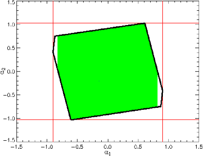
Figure 4: As Fig. 3 but for 3 binned $w$ modes projected onto the plane of the first two PC coefficients. Here we suppress the axes. The light, red vertical and horizontal lines show the mode-by-mode limits; the thick, black polygon defines the exact, pure and complete function space, and the green, shaded region is the global approximation.

While we have solved the problem of obtaining efficiently the constraint on the region of principal component space that is viable given some bounds on the state function, we have to ask whether this is really the best path for analyzing the effect of various state functions. To scan over all viable PCs we would select from the PC coefficients within the allowed region. If the probability of the state function in the bin basis was uniform within the bounds, then because of the linearity of the principal component transformation the interior volume in PC coefficient space can also be uniformly sampled. However, in general we would have some correlation

$$\langle\alpha_{i}\alpha_{j}\rangle=e_{ip}\,e_{jq}\,\langle w_{p}w_{q}\rangle\,,$$ (9)

where angle brackets denote the ensemble average and $p$, $q$ are redshift bin indices (implicitly summed) while $i$, $j$ are component mode indices.

Writing this in matrix notation,

$$A=EWE^{T}\,,$$ (10)

where $W$ is the correlation of the state function (e.g. equation of state values in redshift bins) and $A$ is the correlation that then must be imposed on the selection of PC coefficients. Note that when the bounds on the state function are redshift dependent – as when some data constraint knowledge is incorporated – then even a diagonal $W$ does not lead to a diagonal $A$.

III.2 Restricting Modes

If we keep only $M$ modes in PC space then, because the $\alpha_{i}$ axes are not in general aligned with the bin basis $w_{i}$ axes, the PCs will still span the redshift range but will not be able to describe the full range of $w(z)$ behaviors within the true bounds. That is, we diminish the completeness if we restrict the number of PC modes. Note this can be treated in the hyperrectangle picture as slices through the $N$-rectangle at fixed values of the neglected $N-M$ parameters (see the Appendix for more details). Figure 5 shows an example of the diminished state function space accessed when limiting to 4 modes (out of 17). Moreover, the impurity of the mode-by-mode method becomes more severe, with Fig. 6 showing that using less than the full number of modes can yield up to 70% of the generated forms of the state function being spurious, i.e. ones that invalidly exceed the bounds, under the restriction to the first $M$ modes.

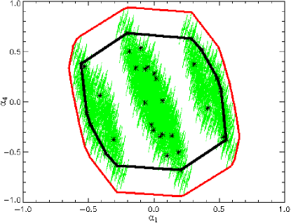
Figure 5: Restricting the number of PC modes kept in the analysis will lose completeness in the state function forms allowed. The light, green dots show the projection of the full set of hyperrectangle corners, with the light, red outer polygon giving the pure and complete bounds in $\alpha_{1}$-$\alpha_{4}$ space. The black dots and black polygon show the case when only the first 4 modes are kept. The region in between the polygons represents viable, but lost state functions.

Figure 6: When not all PC modes are kept then the purity of the mode-by-mode method decreases. The curve shows the range purity – the product of the bounds on each PC coefficient for the exact method when only $M$ modes are retained vs. when all modes are. This is also equivalent to the ratio of the $M$ mode range area to the mode-by-mode method’s area.

In the end, then, because of the coefficient correlations and the completeness issues, little advantage accrues in fact to the use of PCA for the scanning over functional forms. It is more efficient (and innately pure and complete) simply to carry out the analysis in the original state function space where the constraints originated. A standard redshift bin basis allows the freedom needed to model the form of the state function, and the constraints can be imposed naturally without complicating the generation of realizations. In the next sections we demonstrate the real world application of the bin basis state functions to problems involving calculating the effects on cosmology results when confronted with unknown systematics functions.

IV Systematics: Supernova Population Drift

The use of constrained functions, and their impact on parameter estimation or the science results, enters into myriad areas of cosmology. This is a particularly important issue for systematic uncertainties, where we do not know the form of the residual error function. We therefore consider the example of the population fraction of a certain type of source as a key element of the cosmology calculation and take as the state function the uncertainty in our knowledge of it. By definition the function is constrained to take values in the range $[0,1]$. If the source is a standardized distance indicator such as Type Ia supernovae (SN) and we posit that the populations represent subclasses with slightly different intrinsic magnitudes, then any variation with redshift in the population fractions will appear as magnitude evolution and, if unrecognized, bias the cosmological parameter estimation. This is known as population drift (for theoretical discussion and observational limits see coping ; sullivan ; conley07 ; bronder ; howell08 ; sullivan09 ).

In lin0812 , the effects of population drift as a bias or increased dispersion (if adding fit parameters) on cosmology were investigated for a class of state functions depending as a power law in redshift (also see virey ). Here we can analyze every form of population drift and investigate which are the most dangerous. In addition we refine our quantification of the cosmology bias and explore in what redshift ranges the population drift systematic is most biasing.

Population drift as a systematic relies on two elements: an actual difference in intrinsic magnitudes between the subclasses and a redshift dependence in the difference. A mere constant difference is absorbed into the absolute magnitude nuisance parameter $\mathcal{M}$. For simplicity, we illustrate the basic results for a two population model, where the SN have a fraction $f_{1}(z)$ with intrinsic magnitude $M_{1}$ and a fraction $f_{2}(z)$ with intrinsic magnitude $M_{2}$. We can consider $f_{1}$ as representing all the populations we recognize and $f_{2}=1-f_{1}$ as an aggregate of those unrecognized. Then the unrecognized systematics appears as a magnitude evolution

$$\Delta m(z)=\Delta M\,[f(z)-f(0)]\,,$$ (11)

where $\Delta M=M_{2}-M_{1}$ and $f=f_{2}$ is now our state function. The constraint on the state function, by definition of the population fraction, is $f\in[0,1]$.

Propagating this systematic through to the cosmology parameters is straightforward. For a parameter set $\vec{p}=\{p_{i}\}$, the bias is (see, e.g., linbias )

$$\delta\vec{p}=(U^{T}C^{-1}U)^{-1}\,U^{T}C^{-1}\,\Delta O\,,$$ (12)

where $O$ is the observable, $U=\partial O/\partial\vec{p}$, $C$ the error covariance matrix for the observables and $\Delta O$ is a systematic offset in observable $O$. The term in parentheses is simply the Fisher matrix, and so its inverse is the parameter covariance matrix. In the case we are currently considering the observables $O$ are SN magnitudes at various redshifts and $\Delta O$ is the magnitude offset of Eq. (11). For a diagonal error covariance matrix the equation takes a simpler form

$$\delta p_{i}=\Delta M\,(F^{-1})_{ij}\sum_{k=1}^{N}f(z_{k})\frac{1}{\sigma^{2}(m_{k})}\frac{\partial m_{k}}{\partial p_{j}}\,.$$ (13)

Here $F$ is the Fisher matrix, say $4\times 4$ with respect to $\mathcal{M}$, $\Omega_{m}$, $w_{0}$, and $w_{a}$, where $\Omega_{m}$ is the present matter density in units of the critical density. There are $N$ data points, each with an associated redshift $z_{k}$.

We can now explore the effect of any form for $f(z)$, subject only to the constraint $0\leq f(z)\leq 1$. We do not need to assume a functional form for $f$, rather we want to allow it complete freedom under constraint. As we saw in the previous section, no real advantage accrues to a principal component analysis – all the information exists and is more accessible using a redshift bin basis. In fact, PCA when keeping only a more limited number of modes loses information and the bin basis allows for greater efficiency in scanning the allowed state function parameter space.

Before we calculate the bias we examine in more detail how to assess it quantitatively. The bias $\delta p_{i}$ itself is only informative together with the cosmological parameter uncertainties. If the estimated uncertainty on the parameters is large, then the relative effect of a particular bias is lower, meaning that the (mis)estimated model is still within some acceptable confidence level contour. For each parameter $p_{i}$, lin0812 employed the risk statistic kendall

$${\rm Risk}(p_{i})=\sqrt{\sigma_{p_{i}}^{2}+\delta p_{i}^{2}}$$ (14)

as a measure of the influence of the bias. However, the overall cosmology is biased by the vector $\delta\vec{p}$. One could imagine that each parameter bias relative to the dispersion is small, but in a direction such that $\delta\vec{p}$ is oriented along the thin part (minor axis) of the confidence level contour; then a small shift could actually be a large bias relative to the contour, i.e. in terms of the $\Delta\chi^{2}$. Following shapiro (cf. dodelson ) therefore, we use as our bias statistic

$$\Delta\chi^{2}=\boldsymbol{\delta p}\,\mathbf{F}^{(r)}\,\boldsymbol{\delta p}^{T}\,,$$ (15)

where $\boldsymbol{\delta p}$ is the vector of parameter biases we consider and $\mathbf{F}^{(r)}$ is the reduced Fisher matrix, marginalized over all parameters except those in whose biases we are interested. For example, if we consider biases in the $w_{0}$-$w_{a}$ contour, then $\mathbf{F}^{(r)}$ is the inverse of the $2\times 2$ submatrix of the covariance matrix containing $w_{0}$ and $w_{a}$. In the case of a single parameter, $\Delta\chi^{2}=(\delta p/\sigma_{p})^{2}$ and Risk $=\sigma_{p}\sqrt{1+\Delta\chi^{2}}$.

We can now scan over all possible population drifts $f(z)-f(0)$ and evaluate the bias effects on the cosmological parameters. We write $f$ in the redshift bin basis, initially with 17 bins uniform between $z=0-1.7$. For the Fisher matrix we take simulated data based on the SNAP SN redshift and error distribution snap , plus a Planck-inspired constraint on the reduced distance to CMB last scattering of 0.2%. The fiducial cosmology is $\Lambda$CDM with matter density $\Omega_{m}=0.28$.

Table 1 describes the population evolution functions computed to deliver the maximum bias in $\Delta\chi^{2}$. The results have a very simple form: a single or double sharp transition in redshift. This can be understood through analyzing Eq. (13). The bias is a linear transformation of $f$, hence for a maximum bias $f$ is driven to the extreme value that complements the sign of the term $\beta_{i}\equiv(F^{-1})_{ij}\,\partial m_{k}/\partial p_{j}$, for each $z_{k}$. To maximize $\delta p_{i}$, when $\beta_{i}>0$ then $f$ should be 1, while when $\beta_{i}<0$ then $f$ should be 0. This will give coherent addition of the terms in the sum and so deliver the largest $\delta p_{i}$. Thus $f$ should simply be a series of tophats over those redshifts where $\beta_{i}(z_{k})$ is positive. For the parameter $\Omega_{m}$, $\beta_{\Omega_{m}}$ crosses once through 0 so $\delta\Omega_{m}$ is maximized by a population function that has a single transition, at $z\approx 0.7$. Thus the most potent evolution function $f$ – the one having the strongest consequence for cosmology estimation – has a step appearing at $z=0.7$ and extending to the maximum redshift. For $w_{0}$ or $w_{a}$, the respective $\beta$’s cross twice through 0 so $f$ forms a tophat extending from $z\approx 0.2$ (respectively 0.1) to $z\approx 1.0$.

Parameters	$z_{\rm trans}$	max $\Delta\chi^{2}_{\Delta M=0.01}$	$\Delta M\,(1\,\sigma)$
$\Omega_{m}$	0.7	$0.92$	$0.010$
$w_{0}$	0.2, 1.0	$1.35$	$0.0086$
$w_{a}$	0.1, 1.0	$1.35$	$0.0086$
$w_{0},w_{a}$	0.1, 1.0	$1.36$	$0.013$
$\Omega_{m},w_{0},w_{a}$	0.1, 0.9	$1.39$	$0.016$

Table 1: For each set of parameters we consider the form of population evolution that maximizes the cosmology bias in terms of $\Delta\chi^{2}$. The $z_{\rm trans}$ column gives the redshift of the maximizing step function in $f$, delivering a maximum bias $\Delta\chi^{2}$ scaled to the case where $\Delta M=0.01$, shown in the next column. Note $\Delta\chi^{2}$ will scale as $\Delta M^{2}$. The last column shows the value of $\Delta M$ that will shift the derived cosmology by $1\sigma$ from the true cosmology.

This has a number of crucial implications. First, since the state function with the maximal effect arises from a sharp transition, we see that it was prescient to use the bin basis for the population function. Had we transformed to principal component space, or some smooth orthogonal basis such as the Chebyshev polynomials considered by lin0812 ; amara , then we would have had difficulty approximating the true solution with a finite number of modes. Second, the sensitivity to population evolution at specific redshifts guides the survey design to obtain especially detailed measurements at these redshifts. The results indicate that as observations make the transition from local ($z<0.1$) SN to low redshift ($z\gtrsim 0.2$) SN, they must comprehensively collect and study the SN properties so as to ensure a firm like-to-like comparison and not allow for unrecognized populations. Similarly, the transition from $z<1$ to $z>1$ SN is key, so a transition from ground-based observing to the space-based observing necessitated at $z>1$ could be problematic. A homogeneous survey extending across this transition would have far better control over the systematic uncertainty.

These results hold as well when considering simultaneously bias in multiple parameters in the $\Delta\chi^{2}$ formalism. The population $f$ enters Eq. (15) quadratically and so the bias is still maximized by the extreme values of $f$, i.e. top hats in redshift. The transition locations do not shift appreciably when considering bias in the two parameter space of $w_{0}$-$w_{a}$ nor the three parameters $\Omega_{m}$, $w_{0}$, $w_{a}$ simultaneously. Furthermore, the transition locations are robust to changing the step functions to more gradual slopes.

The last column of Table 1 shows the magnitude of $\Delta M$ that in the worst case of population evolution causes a $1\sigma$ misestimation of the cosmology. This is where the scaling of the state function bounds enters: the shape, i.e. redshift dependence of the population function, is unaffected by amplitude of the bounds, but the absolute level is determined by the bounds. If we consider twice as large values for $\Delta M$ (or if we were to unphysically allow $f$ to range from 0 to 2), then $\Delta\chi^{2}$ just scales with $\Delta M^{2}$. If we want to be sure that population drift cannot cause a $>1\sigma$ shift in the equation of state parameters, we need to be able to recognize SN subclasses differing by 0.0086 mag or more.

Figure 7 shows the relation between the maximum number of standard deviations $\sigma$ by which the cosmology is distorted, as a function of difference in absolute magnitudes $\Delta M$ between the populations, for the full set of cosmological parameters. While $\Delta\chi^{2}$ scales as $\Delta M^{2}$, the number of $\sigma$ this bias corresponds to only scales as $\Delta M$ in the one parameter case. We see that for three parameters the $\sigma$ remains nearly linear for large $\Delta M$ but does not improve as rapidly for $\Delta M<0.015$.

Figure 7: For the maximally biasing population drift the cosmological parameter set $\{\Omega_{m},w_{o},w_{a}\}$ is biased by $1\sigma$ for a population magnitude difference $\Delta M=0.016$ mag. The curve shows by how many $\sigma$ the best fit cosmology is biased as a function of $\Delta M$.

Beyond the maximum $\Delta\chi^{2}$, we can investigate other properties of the biasing. For example, we can explore further the direction of the systematic shift caused in the cosmology parameters, the relation of the forms of the population drift, i.e. the number of steps or oscillations, to the bias, and the overall statistics of the biasing.

We begin with the effect on the equation of state estimation caused by the systematic error. Figure 8 shows the specific form of bias induced in the equation of state by the 10 worst case population drifts. The worst biases all distort the cosmology in the same way: making a cosmological constant look like a rapidly varying equation of state. Indeed, this is characteristic not just of population drift but of any sharp transition in the SN magnitudes, such as from patching together two redshift samples with an unrecognized offset (local to low redshift samples, or ground-based to space-based). This points up the need for tight crosscalibration, and ideally a continuous, homogeneous data set, as well as the need for caution in interpreting an apparent behavior of the equation of state crossing $w=-1$: exactly what is expected from such a systematic.

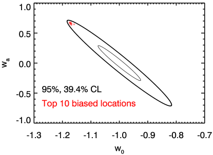
Figure 8: The biases induced for $\Delta M=0.02$ by the worst population evolution functions – those that induce the 10 largest $\Delta\chi^{2}$ – are plotted in the $w_{0}$-$w_{a}$ plane as x’s. Note how they congregate at the extreme end of the major axis of the confidence contour. The inner ellipse indicates the 39% confidence level contour (so $\sigma(w_{0})$, $\sigma(w_{a})$ are given by direct projection to the respective axis), while the outer ellipse shows the 95% cl joint likelihood contour.

The influence of the forms of the population evolution function on the bias generated in the cosmology parameters can be investigated through looking at the statistics of the $\Delta\chi^{2}$ distribution. For example, while the maximum bias is generated from a population function with one or two steps at sensitive redshifts, we expect a large number of transitions to have relatively little effect since such an oscillatory behavior does not resemble the effect of a cosmological parameter. The sum of the terms in Eq. (13) effectively cancels out. Thus certain types of systematics are fairly benign, such as quasi-periodic k-correction errors daviskim ; hsiao . Figure 9 shows the range of $\Delta\chi^{2}$ generated as a function of the number of transitions in $f$ between redshift bins. As expected, as the number of transitions gets large, the bias decreases. Similarly, when the step amplitude is small then the bias is negligible so the $\Delta\chi^{2}$ distribution ranges between 0 and the maximum for each number of transitions.

Figure 9: The range of possible biases $\Delta\chi^{2}$ in the cosmology likelihood contour for $\Omega_{m}$-$w_{0}$-$w_{a}$ is plotted vs. the number of transitions (changes in value between the 17 redshift bins) in the population evolution.

The location in redshift of the features in the population function also are important. As we saw in Table 1, $z\approx 0.1$ and $z\approx 1$ were key regions for sensitivity to bias. In Fig. 10 we plot the redshift locations giving not just maximum bias, but greater than a certain percentage of maximum bias (still keeping full steps, i.e. $f=0$ or 1). We see that down to 50% of the maximum possible bias the culprits are still population evolution around these sensitive redshifts. This suggests that surveys designed to recognize population subclasses through especially comprehensive measurements around these redshifts can remove the top half of possible cosmology bias, improving the systematics by a factor two.

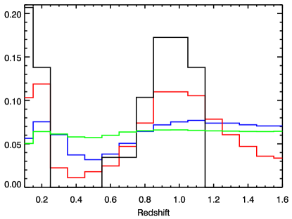
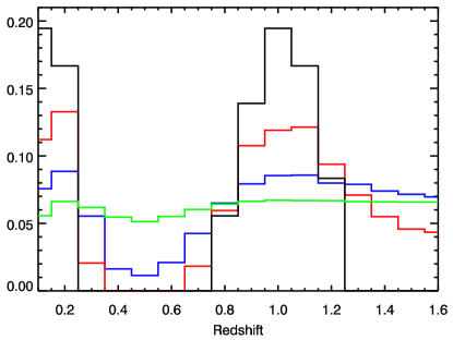
Figure 10: The histograms show the redshift locations of the most sensitive steps in the population function $f$ for various cuts in $\Delta\chi^{2}$. In order from highest to lowest peak the cuts are 90%, 75%, 50%, 25% of the maximum possible $\Delta\chi^{2}$. The top panel considers the $\Delta\chi^{2}$ bias for the cosmology likelihood contour in the $\Omega_{m}$-$w_{0}$-$w_{a}$ space while the bottom panel is for the $w_{0}$-$w_{a}$ space. Note that the most sensitive redshifts are robust to lower levels of bias, down to 50% of maximum, and to the parameter space considered.

If we consider every possible form of the population function, randomly scanning over the number of steps and locations of transitions, then most of these will have little effect on the cosmology. The mean bias, or $\langle\Delta\chi^{2}\rangle$ will therefore be small. For example, the mean is only 0.08 for the $w_{0}$-$w_{a}$ contour. This is simply due to combinatorics: there are many more ways of having, say, 8 steps over 17 bins than 1 step – some 24000 times more possibilities – and multistep functions will have little impact on the cosmology. Furthermore the random location of the steps will also dilute the mean bias. However, random population evolution is not the issue; for survey design we have to consider the worst case scenario, i.e. which systematics can give the most egregious misestimation of the cosmology results, and how to control this. The results indicate that experiments should be guided by requirements to recognize subtypes with magnitude differences down to $\sim 0.01$ mag (Fig. 7), and with particularly comprehensive measurements around $z\approx 0.1$ and $z\approx 1$ (Fig. 10).

V Systematics: Dust Correction and Calibration

The analysis of the constrained state function in terms of population drift was particularly straightforward because of the linear relation between the function $f(z)$ and the observable $m(z)$. To illustrate a more complicated application we consider the systematic uncertainty due to dust extinction correction in supernova distances. This is currently one of the dominant systematics conley ; kowalski ; hicken ; nobili ; goobar09 and uses measurements in multiple wavelength bands, or filters, to correct for the dust effects. However, if the different filters have some uncertainty in their calibrations then this propagates through to the relative fluxes or colors and then to the dust correction kimmiquel . We use a simple, two band version of this as an illustration of a nonlinear, constrained systematic.

We take the systematic to arise from zeropoint calibration errors in each filter, and the constraint can arise from subsidiary measurements such as on standard stars or instrumental calibration (see, e.g., stubbs ) that limit the zeropoint offsets to lie within $\Delta Z\in[Z_{-},Z_{+}]$. Again, it is the relative zeropoint differences, or colors, that cause bias; uniform offsets do not affect cosmology. Because the flux from sources at different redshifts peaks in different wavelength bands, the zeropoint errors will induce a redshift dependent error in the magnitude and hence a bias in the cosmology parameter estimation. In addition, because the use of multiple bands to define the dust correction leads to an interdependence of SN at different redshifts, a correlated error matrix enters kimmiquel .

In the two band toy model for dust correction, the corrected magnitude $\tilde{m}$ is related to the magnitudes measured in two neighboring bands by

$$\tilde{m}_{i}=(1+R)\,m_{i}-R\,m_{i+1}\,,$$ (16)

where $R$ is the extinction ratio. We use as the two bands the restframe $B$ and $V$ bands for each supernovae, take $R=2.1$ (somewhat emphasizing the effect), and consider only calibration zeropoint error contributions to the dust correction, not any intrinsic SN color variation. This simple model is sufficient to illustrate the effects of a nondiagonal error covariance matrix

$$C = BEB^{T}$$ (17)

$$B = (1+R)\,\delta_{ij}-R\,\delta_{i,j-1}\,,$$ (18)

where $E$ is the pre-correction, possibly diagonal, error covariance matrix.

The Fisher matrix is formed using the nondiagonal error covariance matrix $C$ and we then calculate the parameter bias due to zeropoint offsets $\Delta Z_{k}$ in the magnitudes by means of Eq. (12). We consider 8 filters logarithmically spaced in wavelength, with centers at $\lambda_{0}\,(1+a_{\star})^{k-1}$, for $k=1-8$, taking $\lambda_{0}=4400$Å and $a_{\star}=0.15$ so the maximum redshift corresponds to 1.66 omnibus . Our state function is $\Delta Z$, which can be both positive and negative within the bounds, and we scan over all possible forms within the bounds and analyze the cosmology bias.

Table 2 presents the results in the same format as the previous case in Table 1. However here the steps are in band zeropoints not population fractions and the locations are listed in terms of the filter numbers. The important quantity is $\Delta Z_{\rm rel}$ between filters (recall that an overall zeropoint error has no cosmology effect), and needs to be constrained to the $\sim 0.01$ level. The furthest red filters, used for the highest redshift SN, are among the most sensitive to bias and should be tightly calibrated with instrumental and standard star measurements.

Parameters	Transitions	max $\Delta\chi^{2}_{\Delta Z=0.01}$	$\Delta Z_{\rm rel}\,(1\sigma)$
$\Omega_{m}$	2-3, 7-8	$4.07$	0.0098
$w_{0}$	1-2, 4-5, 7-8	$2.79$	0.012
$w_{a}$	1-2, 4-5, 7-8	$2.99$	0.012
$w_{0},w_{a}$	3-4, 7-8	$4.12$	0.015
$\Omega_{m},w_{0},w_{a}$	3-4, 7-8	$4.55$	0.018

Table 2: For each set of parameters we consider the form of filter zeropoint errors that maximize the bias in terms of $\Delta\chi^{2}$. The transitions column gives the filter transitions of the maximizing function in $\Delta Z$, delivering a maximum bias $\Delta\chi^{2}$ scaled to the case where the zeropoint calibration is bounded by $|\Delta Z|=0.01$, shown in the next column. The last column shows the value of $\Delta Z_{\rm rel}$ between two filters that will shift the derived cosmology by $1\sigma$ from the true cosmology.

As in the previous case in Sec. IV, the shape, i.e. wavelength dependence of the zeropoint calibration, is unaffected by amplitude of the bounds on the calibration state function, but the absolute level is determined by the bounds. If we consider twice as large values for $\Delta Z$, then $\Delta\chi^{2}$ just scales with $\Delta Z^{2}$.

Any filter zeropoint step affects SN in some redshift range, and hence the overall cosmology. Thus an improvement in the knowledge of a filter offset $\Delta Z_{k}$ reduces the maximum $\Delta\chi^{2}$ bias. Figure 11 shows the effect of more tightly calibrating a given filter. We see the greatest improvement for the end bands – which are used for the lowest redshift, anchoring SN and the highest redshift, lever-arm SN – and the middle bands, which are used near the sensitive $z\approx 1$ region. Thus survey design that provides particularly comprehensive calibration for these bands will see a large payoff in systematics control.

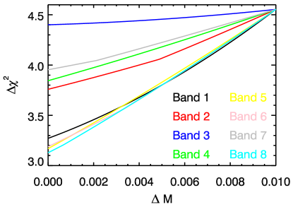
Figure 11: The maximum $\Delta\chi^{2}$ bias is plotted as a function of the bound on individual filter band zeropoint offsets. The greatest improvement in systematics control comes from improving the calibration uncertainty $\Delta Z$ for bands 1, 5, 6, 8 which correspond to the most cosmologically sensitive redshift leverages, near $z\approx 0$, $1$, $1.7$.

VI Conclusions

Modeling unknown functions in cosmology is pervasive, whether these are functions that carry the physics we are directly interested in, such as the dark energy equation of state history, or functions describing subsidiary effects that we wish to subtract out, such as intermediate astrophysics or modeling of uncertainties. If the functional form is assumed, then this becomes parameter fitting or “self-calibration” but it is interesting and important to investigate the results when any viable function is allowed. The viability is subject only to some constraints placed on the bounds of the function through theoretical or measurement input.

We investigated two main issues for cosmological analysis in the presence of unknown but constrained functions. First, we demonstrated a computationally efficient, pure and complete method for determining the viable space of principal component coefficients, with a simple geometric picture in terms of a hyperrectangle in the $N$-dimensional basis space. This improves on the efficiency of the previous mode-by-mode method by a factor 3, while guaranteeing purity, i.e. validity of the selected functions. Conversely, compared to the also pure and complete direct scanning method, the projected hyperrectangle method gains in efficiency by factors of $10^{10}$ or greater.

For many astrophysical problems the orthogonal bin basis (in redshift or wavelength) is well suited. We evaluated two “real world” systematics issues with this method, one in redshift and one in wavelength. The first dealt with unrecognized population evolution in a subclass of standard candles. Rather than assuming a form of evolution we analyzed the effects of all possible functional forms lying within some bounds. The results provide quantitative guidance to controlling the worst cosmology biases arising from the systematic uncertainties. In particular, we find that the regions $z\approx 0.1$ and $z\approx 1.0$ can benefit most from comprehensive observations to limit unrecognized subclasses (at the $\sim 0.01$ mag level); surveys homogeneous over these redshift regions have improved control over cosmology misestimation.

The second application concerned dust extinction corrections for Type Ia supernovae, where measurements in multiple wavelength bands can fit for dust but also correlate supernovae at different redshifts. We analyzed the case where systematic uncertainties existed in the filter calibrations, bounded by instrumental or standard star observations, and propagated all possible functional forms into cosmology biases. Again we found which specific forms were most damaging and that measurements designed to control such errors could remove the worst biases. In particular, those bands used for the lowest and highest supernovae, and ones relevant around $z\approx 1.0$, should be most comprehensively calibrated (to the $\sim 0.01$ mag level relatively) for a more robust survey.

Appendix: Efficient Projection and Boundary Definition

Since the dark energy physics of interest mostly translates into descriptions of the EOS in redshift bin space, our bounds on the state function are given in this space. In this Appendix we will detail, through a geometrical understanding, a fast method for analyzing how these bounds in bin space may be carried into bounds on coefficients in principal components space. The bounds on $w(z)$ directly form the space of the permitted sets of these coefficients, but picking a pure and complete set of coefficients in PC space is not so simple.

The value for the EOS, say, at a particular redshift $z$ is not described by just one mode as in the bin space case, but by a linear combination of many modes weighted by their respective coefficients. To scan the whole coefficient space within the bounds given in redshift space requires an impractical amount of computational power, as discussed in Sec. II. We need a more clever method of obtaining the desired results.

For a set of independent state function bounds on $\{w_{i}\}$, the permitted space in bin space is bounded by a hyperrectangle, or orthotope. The coordinates of the corners are given by any combination $W_{1}^{\pm},W_{2}^{\pm},\dots,W_{N}^{\pm}$ where $W_{i}^{\pm}$ denotes the maximum and minimum values allowed for bin $i$, and $N$ is the number of bins. This fixes the $2^{N}$ corners. This orthotope structure contains all the needed information on the boundary of the allowed space no matter the basis.

Let us first address how to determine the viable region for any set of principal component coefficients, $\alpha_{1},\dots,\alpha_{m}$. The permitted space is simply the projection of the orthotope onto the subspace spanned by these components. The nodes of the boundary in PC space are found by projecting the vectors going from the origin to the corners of the orthotope. Denoting these ($N$-dimensional) vectors as $\mathbf{c_{i}}$ and the projected ($m$-dimensional) node vectors in the $\mathbf{S}=[e_{1},\dots,e_{m}]$ PC space as $\mathbf{p_{i}}=(p_{i1},\dots,p_{im})$, where $p_{i1},\dots,p_{im}$ are the coordinates of $\mathbf{p_{i}}$ with respect to the axes $\alpha_{1},\dots,\alpha_{m}$, we find

$$\mathbf{p_{i}}=(\mathbf{S}^{T}\mathbf{S})^{-1}\mathbf{S}^{T}\mathbf{c_{i}}\,.$$ (19)

Consider now the case where we keep only a subset of PC modes, i.e. we do not marginalize over the other modes but fix their coefficients, e.g. to 0. Information is lost by not using the complete basis in the expansion, but sometimes data or practicalities do not enable us to know or measure all modes. Therefore, we must sometimes sample with only a subset $M$ of modes. The new permitted space of PC coefficients is the intersection of the $M$-dimensional space with the original $N$-dimensional space. This subspace is completely defined by the boundary points, found by looking at the intersections between the $M$-dimensional space of interest and the $N$-dimensional bounded bin space (cf. the black dots in Fig. 5). However, the allowed space is not generally a $M$-rectangle; for example, a plane cutting through a cube can have a boundary with six corners unless it is specially oriented. This has the consequence that there is no $M$-dimensional basis that will generally be pure and complete (i.e. there are no orthogonal axes spanning the space). Only the original bin basis in $N$-dimensions can provide a pure and complete description of the valid state functions.

To describe the actual procedure for evaluating the allowed region in PC space we rephrase the issue more mathematically. The determination of the coefficient bounds is solved by considering the intersection of the subspace $\mathbf{C_{a}}$, spanned by the principal components keeping the selected number of coefficients constant, with the orthotope. In the $3$ dimensional case, with a 2 dimensional subspace, the boundaries are of $3-2$ dimensions, i.e. lines, having parametric form $\mathbf{I}_{a}+(\mathbf{I}_{b}-\mathbf{I}_{a})t$ and the plane is parameterized by $\mathbf{P}_{0}+(\mathbf{P}_{1}-\mathbf{P}_{0})u+(\mathbf{P}_{2}-\mathbf{P}_{0})v$, where $t$, $u$, $v$ are real numbers, and $\mathbf{I}_{i}$ and $\mathbf{P}_{j}$ are points on the line and in the plane, respectively. Setting $\mathbf{D}=[\mathbf{I}_{a}-\mathbf{P}_{0}]$, $\mathbf{A}=[\mathbf{I}_{a}-\mathbf{I}_{b},\mathbf{P}_{1}-\mathbf{P}_{0},\mathbf{P}_{2}-\mathbf{P}_{0}]$, and $\mathbf{L}=[t,u,v]$ we find

$$\mathbf{D^{-1}A=L}\,.$$ (20)

In the higher dimensional case the solution has the identical form. Geometrically, $\mathbf{I}$ represents vectors going from the origin to the corners of the orthotope (so $t\in[0,1]$) and $\mathbf{P}$ are non-colinear points in $\mathbf{C_{a}}$. The matrix manipulations can be computed easily so solving for the allowed region in PC space is highly efficient and quick.

References

- (1) R. de Putter & E.V. Linder, JCAP 0810, 042 (2008) [arXiv:0808.0189]
- (2) D. Huterer & G. Starkman, Phys. Rev. Lett. 90, 031301 (2003) [arXiv:astro-ph/0207517]
- (3) D. Huterer & A. Cooray, Phys. Rev. D 71, 023506 (2005) [arXiv:astro-ph/0404062]
- (4) R. de Putter & E.V. Linder, Astropart. Phys. 29, 424 (2008) [arXiv:0710.0373]
- (5) M.J. Mortonson, W. Hu, D. Huterer, Phys. Rev. D 79, 023004 (2009) [arXiv:0810.1744]
- (6) T.D. Kitching & A. Amara, MNRAS 398, 2134 (2009) [arXiv:0905.3383]
- (7) M.J. Mortonson, arXiv:0908.0346
- (8) M.J. Mortonson & W. Hu, ApJ 672, 737 (2008) [arXiv:0705.1132]
- (9) E.V. Linder, Phys. Rev. D 79, 023509 (2009) [arXiv:0812.0370]
- (10) T.D. Kitching, A. Amara, F.B. Abdalla, B. Joachimi, A. Refregier, MNRAS 399, 2107 (2009) [arXiv:0812.1966]
- (11) D. Branch, S. Perlmutter, E. Baron, P. Nugent, arXiv:astro-ph/0109070
- (12) M.Sullivan et al., ApJ 648, 868 (2006) [arXiv:astro-ph/0605455]
- (13) D.A. Howell, M. Sullivan, A. Conley, R.G. Carlberg, ApJ 667, L37 (2007) [arXiv:astro-ph/0701912]
- (14) T.J. Bronder et al., A&A 477, 717 (2008) [arXiv:0709.0859]
- (15) D.A. Howell et al., ApJ 691, 661 (2009) [arXiv:0810.0031]
- (16) M. Sullivan et al., ApJ 693, L76 (2009) [arXiv:0901.2476]
- (17) S. Linden, J-M. Virey, A. Tilquin, A&A 506, 1095 (2009) [arXiv:0907.4495]
- (18) E.V. Linder, Astropart. Phys. 26, 102 (2006) [arXiv:astro-ph/0604280]
- (19) M.G. Kendall, A. Stuart, J.K. Ord, Advanced Theory of Statistics (Oxford U. Press: 1987)
- (20) C. Shapiro, ApJ 696, 775 (2009) [arXiv:0812.0769]
- (21) S. Dodelson, C. Shapiro, M. White, Phys. Rev. D 73, 023009 (2006) [arXiv:astro-ph/0508296]
- (22) A.G. Kim, E.V. Linder, R. Miquel, N. Mostek, MNRAS 347, 909 (2004) [arXiv:astro-ph/0304509]
- (23) T.M. Davis, B.P. Schmidt, A.G. Kim, PASP 118, 205 (2006) [arXiv:astro-ph/0511017]
- (24) E.Y. Hsiao et al., ApJ 663, 1187 (2007) [arXiv:astro-ph/0703529]
- (25) A. Conley et al., ApJ 664, L13 (2007) [arXiv:0705.0367]
- (26) M. Kowalski et al., ApJ 686, 749 (2008) [arXiv:0804.4142]
- (27) M. Hicken et al., ApJ 700, 1097 (2009) [arXiv:0901.4804]
- (28) S. Nobili et al., ApJ 700, 1415 (2009) [arXiv:0906.4318]
- (29) J. Nordin, A. Goobar, J. Jonsson, JCAP 0802, 008 (2008) [arXiv:0801.2482]
- (30) A.G. Kim & R. Miquel, Astropart. Phys. 24, 451 (2006) [arXiv:astro-ph/0508252]
- (31) C.W. Stubbs et al., ASP Conf. Series 364, 373 (2007) [arXiv:astro-ph/0609260]
- (32) G. Aldering et al., arXiv:astro-ph/0405232