A Low-Overhead Energy Detection Based Cooperative Sensing Protocol for Cognitive Radio Systems

Abstract

Cognitive radio and dynamic spectrum access represent a new paradigm shift in more effective use of limited radio spectrum. One core component behind dynamic spectrum access is the sensing of primary user activity in the shared spectrum. Conventional distributed sensing and centralized decision framework involving multiple sensor nodes is proposed to enhance the sensing performance. However, it is difficult to apply the conventional schemes in reality since the overhead in sensing measurement and sensing reporting as well as in sensing report combining limit the number of sensor nodes that can participate in distributive sensing. In this paper, we shall propose a novel, low overhead and low complexity energy detection based cooperative sensing framework for the cognitive radio systems which addresses the above two issues. The energy detection based cooperative sensing scheme greatly reduces the quiet period overhead (for sensing measurement) as well as sensing reporting overhead of the secondary systems and the power scheduling algorithm dynamically allocate the transmission power of the cooperative sensor nodes based on the channel statistics of the links to the BS as well as the quality of the sensing measurement. In order to obtain design insights, we also derive the asymptotic sensing performance of the proposed cooperative sensing framework based on the mobility model. We show that the false alarm and mis-detection performance of the proposed cooperative sensing framework improve as we increase the number of cooperative sensor nodes.

I Introduction

Cognitive radio and dynamic spectrum access are important emerging technologies [1, 2, 3] which may represent a new paradigm shift in more effective use of limited radio spectrum. For instance, some of the license spectrum (such as UHF/VHF band) is under-utilized [4, 5] and this motivated the standardization of Wireless Regional Area Network (WRAN) in IEEE 802.22 [6] to exploit unused spectrum dynamically. One important technical challenge in realizing the vision of cognitive radio systems is to maintain and control potential interference to primary users in the licensed spectrum [7, 8]. There are in general two approaches in cognitive radio systems to realize efficient spectrum sharing, namely a static approach and a dynamic approach. In the static approach (more conservative), the transmit power of the secondary system is limited such that the worst case interference to the primary users is controlled to an acceptable target [9, 10] (protection contour) regardless of the instantaneous activity of the primary system. While this approach is simple, it failed to exploit the dynamic activity and the location of the primary users. In the dynamic approach, the secondary system will sense the activities of the primary system and transmits only during the activity gaps of the primary system. This approach allows better utilization of the shared spectrum especially when the primary system has bursty traffic. As a result, this dynamic approach is commonly adopted as the basic framework in cognitive radio systems.

One core component behind dynamic spectrum access is the sensing of primary user activity in the shared spectrum. For instance, the accuracy of sensing reports from secondary nodes are critical to the functioning of the cognitive radio systems. Imperfect sensing may cause either false alarm or mis-detection problems. When we have false alarm in the sensing report, the secondary system will be over-conservative because it falsely assumed the primary user is active. When we have mis-detection in the sensing report, the secondary system may induce strong interference to the primary users in the shared spectrum. In practice, providing an accurate sensing measurement on the activity of primary users may be challenging for the following reasons. For instance, the secondary system may not have knowledge of the signal structure as well as channel states of the primary users. Hence, the sensing detection is usually done in a non-coherent manner [11, 12]. In addition, in order to maintain a reasonably low interference level to primary system, the secondary nodes shall be able to detect the existence of very weak primary signals [11, 12]. To improve the accuracy of the dynamic spectrum sensing, classical detection theory suggests that the sensing performance can be improved by increasing the sensing time [12, 13, 14]. The sensing performance can be further enhanced by distributive sensing involving multiple sensor nodes. In [15, 16, 17, 18, 19], a distributed sensing and centralized decision framework has been proposed. In [16], each sensor node makes a hard-decision on the primary user activity and feedback the local decisions to the base station. The base station (BS) makes a final decision by majority voting. In [17], the authors proposed a similar framework except that each sensor node feedback the soft sensing measurement and combined at the BS. This framework is also adopted in the IEEE 802.22 sensing architecture. In [12], an asymptotic relationship between the target non-coherent sensing performance and the number of sensing samples needed was derived in the low SNR regime. In [18, 19], the authors proposed type-based distributed sensing schemes for the multi-access channels as well as wireless sensor networks.

While distributive sensing is a promising solution to enhance the sensing performance in cognitive radio systems, there are several important open issues to be addressed as elaborated below.

• Overhead in sensing measurement and sensing reporting In the above works, the overheads in sensing measurement and sensing reporting were ignored. For instance, in 802.22 systems, the BS shall poll a consumer premise equipment (CPE) to perform sensing measurement and report the sensing result in a round robin fashion. Yet, each sensing measurement incur system overhead in the sense that the entire secondary system has to remain silent during the sensing measurement. In addition, reporting of sensing results reliably requires additional overheads. In fact, the issue of sensing report overhead is not too related to hard-decision or soft-decision. Previous literatures have assumed that the reporting links are perfect and the one-bit hard decision result can be delivered to the BS perfectly. However, in practical systems, to reliably deliver one-bit sensing information (even for hard decision) actually involves a lot of overheads, including reliable channel coding, packet preamble, CRC checking bits etc. Moreover, if we allow all the primary detected sensor nodes to report the sensing measurement simultaneously, the BS may not be able to separate them since the packet collision may happens. In other words, the sensing measurement report (BLM-REP) messages from various sensors have to be delivered to the BS sequentially. Typical ways to enforce this is for the BS to poll the CPEs to report sensing measurement as implemented in the 802.22.

• Overhead in sensing report combining In all the above works, the BS has to combine a large number of distributive sensing measurements from secondary CPEs in the cognitive radio systems. This will incur storage issues as well as the processing complexity which scales linearly with the number of sensing measurements.

Recent discoveries propose pioneering methods to reduce the potential overhead based on the threshold-based cooperative sensing [20, 21] or sequential detection [22, 23] and to improve the throughput of the cognitive transmission [24, 25], but the reporting link is assumed to be perfect which is in general difficult to implement in practical systems. In [26, 27], the authors considered the imperfect reporting channels and the energy detection problem with AWGN reporting channel is addressed in [28]. In this paper, we shall propose a low overhead and low complexity energy detection based cooperative sensing framework for the cognitive radio systems which addresses the above issues. The proposed framework consists of two parts, namely the cooperative sensing scheme and the power scheduling algorithm. The cooperative sensing scheme greatly reduces sensing reporting overhead of the secondary systems. Unlike conventional distributive sensing schemes, the required sensing reporting overhead do not scale with the number of cooperative sensor nodes. Furthermore, the BS does not need extra complexity in combining multiple sensing reports from the cooperative sensor nodes. The power scheduling algorithm dynamically allocates the transmission power of the cooperative sensor nodes based on the channel statistics of the links to the BS as well as the quality of the sensing measurement. In order to obtain design insights, we also derive the asymptotic sensing performance of the proposed cooperative sensing framework based on the mobility model. We show that the false alarm and mis-detection performance of the proposed cooperative sensing framework improve as we increase the number of cooperative sensor nodes. In the low SNR region, to achieve a target false alarm and mis-detection probability, the number of sensor nodes required scales in the order of $\mathcal{O}\big{(}\Sigma_{r}(1+\sqrt{1+\Sigma_{s}})^{2}/\rho_{r}^{2}\rho_{s}^{2}\big{)}$ where $\rho_{r},\Sigma_{r}$ represents the mean and variance of the average received SNR of the “sensor node”-“BS” links and $\rho_{s},\Sigma_{s}$ represents the mean and variance of the average received SNR for the “primary user”-“sensor node” links respectively. We also compare our proposed cooperative sensing scheme with conventional distributive sensing schemes. Under similar system overhead, the proposed scheme can have substantial performance enhancement and has important practical significance.

The rest of the paper is organized as follows. Section II introduces the system model. In Section III, we outline the low-overhead cooperative sensing scheme for cognitive radio systems and discuss the problem formulation of the power allocation in Section IV. We propose our power allocation algorithm by solving the optimization problem in Section V and derive the asymptotic performance analysis in Section VI. In Section VII, we give some numerical results and discussions. Conclusions are given in Section VIII.

II System Model

In this section, we shall elaborate on the channel model of the proposed energy detection based cooperative sensing framework. Consider a cognitive radio system with a single BS of secondary system and multiple sensor nodes as shown in Fig. 1. Each node is equipped with single antenna. To make it precise, we consider a cognitive radio system containing $K$ sensor nodes, each making observations on a deterministic source signal $\theta$ of the primary user within the licensed spectrum, where $\theta=1$ when the primary user is active and $\theta=0$ otherwise. For notation convenience, we define the $k^{th}$ sensing link to be the channel between the primary user and the $k^{th}$ sensor node and define the $k^{th}$ reporting link to be the channel between the $k^{th}$ sensor node and the BS as shown in Fig. 1.

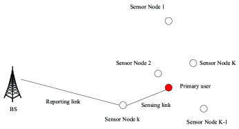
Figure 1: System model of the proposed cooperative sensing framework in the cognitive radio systems.

Denote $h_{k}^{s}$ to be the channel coefficient of the $k^{th}$ sensing link. Each sensor node observes for $T$ units of time and the time average received signal power can be described by

$$|x_{k}|^{2}=\frac{1}{T}\int_{t=0}^{T}{\big{|}h_{k}^{s}\theta x_{p}\sqrt{P_{pu}}+n_{k,t}^{s}\big{|}}^{2}\textrm{d}t$$ (1)

where $h_{k}^{s}$ are Rayleigh fading coefficients with zero mean and variance $\Sigma_{k}^{s}$, $x_{p}$ denotes the transmitted symbols of the primary user with normalized power and $P_{pu}$ denotes the transmitted power by the primary user. The noise $n_{k,t}^{s}$ is additive complex Gaussian random variable with zero mean and normalized variance.

Denote $h_{k}^{r}$ to be the channel coefficient of the $k^{th}$ reporting link and $\mathcal{X}_{k}$ to be the transmitted signal at the $k^{th}$ sensor node. The corresponding received signal at the BS is given by

$$Y=h_{k}^{r}\mathcal{X}_{k}+n_{r}$$ (2)

where $n_{r}$ is additive complex Gaussian random variable with zero mean and normalized variance, and $h_{k}^{r}$ are Rayleigh fading coefficients with zero mean and variance $\Sigma_{k}^{r}$.

The following assumptions are made through the rest of the paper. Firstly, the $k^{th}$ sensor node has perfect instantaneous channel state information (CSI) knowledge of the $k^{th}$ reporting link through the transmitted preamble by the BS. Secondly, we assume the BS only has statistical information (variances of the CSI) of the reporting links and the sensing links.

III Cooperative Sensing Scheme

In this section, we shall describe the low overhead and low complexity energy detection based cooperative sensing scheme. For easy illustration, we first define the observation chances and the static period as follows. An observation chance is defined to be the time duration which allows all the sensor nodes to perform sensing and reporting for one time. A static period is defined to be the period when the channel statistics of the sensing links $\{\Sigma_{k}^{s}\}$ and the reporting links $\{\Sigma_{k}^{r}\}$ remain the same, which contains many observation chances as shown in Fig. 2.

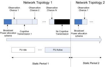
Figure 2: A timing diagram comparison for the static period and the observation chance.

Consider a BS monitoring the behavior of the primary user with the help of $K$ sensor nodes. During each static period, the BS shall sense the primary user activity on the current channel. The proposed cooperative sensing scheme can be briefly described as follows.

Step 1

In each static period, the BS shall determine the optimal power allocation scheme and the corresponding threshold based on the channel statistics of the reporting links and the sensing links. Before the BS of the secondary system transmits, it shall broadcast the downlink sensing request message (the power allocation scheme shall be only broadcast once for each static period and the preamble shall be delivered for each observation chance) to $K$ sensor nodes.

Step 2

Upon receiving the request message, each sensor node shall sense the activity of the primary user for $T$ units of time and obtain a local sensing measurement of $|x_{k}|^{2}$ and the instantaneous CSI knowledge of the reporting link from the preamble.

Step 3

Using the estimated CSI knowledge between the BS and the sensor nodes, all the $K$ sensor nodes amplify and forward a pre-equalized version of the sensing measurement to the BS. Specifically, the transmitted signal at the $k^{th}$ sensor node, $\mathcal{X}_{k}$, is given by

$$\mathcal{X}_{k}=\textrm{conj}(h_{k}^{r})|x_{k}|^{2}\sqrt{\alpha_{k}}$$ (3)

where $\textrm{conj}(\cdot)$ denotes the complex conjugate operation. The sensing results are then RF combined in the air interface and the observation $X$ at the BS is given by

$$X = \frac{\sum_{k=1}^{K}h_{k}^{r}\mathcal{X}_{k}+n_{r}}{K}$$ (4)

$$= \frac{\sum_{k=1}^{K}|h_{k}^{r}|^{2}|x_{k}|^{2}\sqrt{\alpha_{k}}+n_{r}}{K}$$

where $\alpha_{k}$ stands for the amplify-and-forward (AF) gain of the $k^{th}$ sensor node.

Step 4

Using the observation $X$, the BS shall determine the activity of the primary user. Since the BS only has the statistical information of the reporting links and the sensing links, coherent detection cannot be applied and we consider the envelop detection (energy detection). Specifically, the BS shall compare the observation result $X$ with a threshold $\mathcal{T}_{0}$ and determine the activity of the primary user according to (7)

$$\hat{\theta}=g(X)=\left\{\begin{array}[]{l l}1,&X\geq{\mathcal{T}}_{0}\\ 0,&\textrm{otherwise}\end{array}\right.$$ (7)

Step 5

The BS shall start the transmission in the current static period if the primary user is measured to be idle in the current observation chance and wait for the next observation chance otherwise.

In the current literatures, the conventional distributed sensing scheme requires the BS to poll each of the sensor nodes and collect the corresponding sensing reports in a round robin fashion. The BS shall then combine the sensing reports from different sensor nodes to make the final decision. Fig. 3 compares the timing diagram of the proposed cooperative sensing scheme and the conventional distributed sensing scheme. Comparing with the conventional distributed sensing scheme, the proposed cooperative sensing scheme has the following advantages.

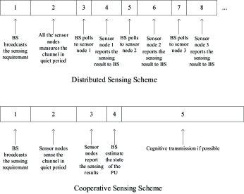
Figure 3: Comparison between the traditional distributed sensing scheme and the proposed cooperative sensing scheme.

• Reduced System Overhead of Reporting. In the conventional distributed sensing scheme, the BS applies the polling scheme to get the reports from multiple sensor nodes. Reporting overhead is proportional to the number of active sensor nodes participating in the sensing. Using the proposed cooperative sensing scheme, the number of active sensor nodes in the cooperative sensing system is no longer limited by the reporting signaling overhead since the sensor nodes in the proposed scheme report the result simultaneously. Hence, the proposed scheme can support much more active sensor nodes than the conventional distributed sensing scheme with the same system overhead.

• Reduced System Overhead in Quiet Period. Using the proposed cooperative sensing scheme, independent measurements from multiple sensor nodes can be exploited. As a result, for the same performance as the conventional distributed sensing scheme, the system quiet period can be substantially reduced.

• Reduced Overhead in Sensing Report Combining. To achieve the benefits of the multiple sensor nodes, the distributed sensing scheme shall combine all the sensing reports from different sensor nodes using Maximum Ratio Combining (MRC). The processing complexity is proportional to the number of sensor nodes in the distributed sensing scheme. Using the proposed cooperative sensing scheme, the MRC is done automatically over the radio interface during the reporting phase of sensing measurement. As a result, no processing complexity at the BS is incurred.

IV Problem Formulation

Based on the proposed energy detection based cooperative sensing scheme, we shall first define the system performance and then formulate the power scheduling problem as a multi-object optimization problem.

IV-A Definition of System Performance

Since the power allocation is done at the BS side, it can only be a function of the statistics of CSI information, i.e. the variances of the reporting links $\{\Sigma_{k}^{r}\}$ and the variances of the sensing links $\{\Sigma_{k}^{s}\}$. For notation convenience, we first have the following definition on power allocation (AF gain) Scheme and the system performance, namely, the probability of mis-detection and the probability of false alarm as follows.

Definition 1 (Power Allocation (AF Gain) Scheme)

A power allocation (AF gain) scheme $\mathbf{a}$ is defined as the AF gain coefficients assigned for $K$ active sensor nodes. Mathematically, the power allocation (AF gain) scheme can be written as $\mathbf{a}=[\alpha_{1},\alpha_{2},\ldots,\alpha_{K}]^{T}$. The power allocation (AF gain) vector $\mathbf{a}$ has to satisfy the following transmission power constraint.

$$\mathbb{E}_{\mathbf{H}}\big{[}|\mathcal{X}_{k}|^{2}\big{]}=\mathbb{E}_{\mathbf{H}}\big{[}|h_{k}^{r}|^{2}|x_{k}|^{4}\alpha_{k}\big{]}\leq P_{k},\ \forall k$$ (8)

where $\mathbf{H}=\{h_{k}^{r},h_{k}^{s}\}$ denotes the instantaneous CSI information of the reporting links and the sensing links.

Definition 2 (Probability of Mis-Detection)

Given the statistics of CSI information $\{\Sigma_{k}^{r},\Sigma_{k}^{s}\}$, the power allocation (AF gain) scheme $\mathbf{a}$ and the threshold $\mathcal{T}_{0}$, the probability of mis-detection is defined to be the probability that the BS cannot detect the transmission of primary user when the primary user is in active state. Mathematically, the probability of mis-detection $P_{MD}$, as a function of power allocation (AF gain) scheme $\mathbf{a}$ and the threshold $\mathcal{T}_{0}$, can be described as

$$P_{MD}(\mathbf{a},\mathcal{T}_{0})=Pr\big{(}\hat{\theta}=0|\theta=1,\{\Sigma_{k}^{r},\Sigma_{k}^{s}\},\mathbf{a},\mathcal{T}_{0}\big{)}$$ (9)

Definition 3 (Probability of False Alarm)

Given the statistics of CSI information $\{\Sigma_{k}^{r},\Sigma_{k}^{s}\}$, the power allocation (AF gain) scheme $\mathbf{a}$ and the threshold $\mathcal{T}_{0}$, the probability of false alarm is defined to be the probability that the BS reports the transmission of primary user erroneously when the primary user is in idle state. Mathematically, the probability of false alarm $P_{FA}$, as a function of power allocation (AF gain) scheme $\mathbf{a}$ and the threshold $\mathcal{T}_{0}$, can be described as

$$P_{FA}(\mathbf{a},\mathcal{T}_{0})=Pr\big{(}\hat{\theta}=1|\theta=0,\{\Sigma_{k}^{r},\Sigma_{k}^{s}\},\mathbf{a},\mathcal{T}_{0}\big{)}$$ (10)

The events of mis-detection and false alarm are undesired in the cognitive radio systems, since the mis-detection causes the interference to the primary user which is not allowed and false alarm reduces the opportunities of utilizing the unoccupied channels. Hence, how to reduce the average probability of mis-detection and false alarm simultaneously is the major objective of this paper. In the next section, we shall formulate the power allocation design into an multi-objective optimization problem.

IV-B Problem Formulation

In order to minimize the average probability of mis-detection and false alarm simultaneously, we shall first calculate the probability of mis-detection and false alarm, which is summarized in the following lemma.

Lemma 1

For sufficiently large $K$ and $T$, the probability of mis-detection and false alarm is given by:

$$Pr\big{(}\hat{\theta}=0|\theta=1,\{\Sigma_{k}^{r},\Sigma_{k}^{s}\},\mathbf{a},\mathcal{T}_{0}\big{)}=Q\big{(}\frac{\mu_{1}-\mathcal{T}_{0}}{\sigma_{1}}\big{)}$$ (11)

$$Pr\big{(}\hat{\theta}=1|\theta=0,\{\Sigma_{k}^{r},\Sigma_{k}^{s}\},\mathbf{a},\mathcal{T}_{0}\big{)}=Q\big{(}\frac{\mathcal{T}_{0}-\mu_{0}}{\sigma_{0}}\big{)}$$ (12)

with

$$\mu_{0} = \frac{\sum_{k=1}^{K}\textrm{SNR}_{k}^{r}}{K}$$

$$\sigma_{0}^{2} = \frac{3\sum_{k=1}^{K}{\textrm{SNR}_{k}^{r,2}}+1}{K^{2}}$$

$$\mu_{1} = \frac{\sum_{k=1}^{K}\textrm{SNR}_{k}^{r}(\textrm{SNR}_{k}^{s}+1)}{K}$$

$$\sigma_{1}^{2} = \frac{3\sum_{k=1}^{K}{\textrm{SNR}_{k}^{r}}^{2}(\textrm{SNR}_{k}^{s,2}+\frac{2}{3}\textrm{SNR}_{k}^{s}+1)+1}{K^{2}}$$

where $\textrm{SNR}_{k}^{s}=P_{pu}\Sigma_{k}^{s}$ denotes the received SNR at the $k^{th}$ node from the primary user, $\textrm{SNR}_{k}^{r}=\sqrt{\alpha_{k}}\Sigma_{k}^{r}$ denotes the ratio of the received signal over the transmitted signal from $k^{th}$ sensor node, and $Q(\cdot)$ denotes the standard Gaussian complementary c.d.f. [29].

Proof:

Please refer to Appendix A for the proof. ∎

Based on the relationship between the system performance (i.e. the probability of missing and false-alarm), the power allocation (AF gain) scheme and the threshold, the optimal power allocation (AF gain) scheme $\mathbf{a}^{*}$ and the optimal threshold $\mathcal{T}_{0}^{*}$ can be described by the following multi-objective optimization problem.

$$(\mathbf{a}^{*},\mathcal{T}_{0}^{*}) = \arg\min_{(\mathbf{a},\mathcal{T}_{0})}\left(\begin{array}[]{l}P_{MD}\big{(}\mathbf{a},\mathcal{T}_{0}\big{)}\\ P_{FA}\big{(}\mathbf{a},\mathcal{T}_{0}\big{)}\end{array}\right)$$ (15)

$$= \arg\min_{(\mathbf{a},\mathcal{T}_{0})}\left(\begin{array}[]{l}Q\big{(}\frac{\mu_{1}-\mathcal{T}_{0}}{\sigma_{1}}\big{)}\\ Q\big{(}\frac{\mathcal{T}_{0}-\mu_{0}}{\sigma_{0}}\big{)}\end{array}\right)$$ (18)

V Power Scheduling Algorithm

In this section, our target is to find the optimal power allocation scheme based on solving the optimization problem given by (18). To measure the efficiency of the multi-objective situation, Pareto Optimality, is widely used to describe those tradeoff relations. A solution can be considered Pareto optimal if there is no other solution that performs at least as good on every criteria and strictly better on at least one criteria. Mathematically, $(\mathbf{a}^{*},\mathcal{T}_{0}^{*})$ is Pareto optimal if we cannot find a solution $(\hat{\mathbf{a}},\hat{\mathcal{T}_{0})}$ such that

$$\left(\begin{array}[]{l}P_{MD}\big{(}\hat{\mathbf{a}},\hat{\mathcal{T}_{0}}\big{)}\\ P_{FA}\big{(}\hat{\mathbf{a}},\hat{\mathcal{T}_{0}}\big{)}\end{array}\right)\preceq\left(\begin{array}[]{l}P_{MD}\big{(}\mathbf{a}^{*},\mathcal{T}_{0}^{*}\big{)}\\ P_{FA}\big{(}\mathbf{a}^{*},\mathcal{T}_{0}^{*}\big{)}\end{array}\right)$$ (23)

where $\preceq$ denotes the element-wise inequality. As a result, we solve the multi-objective optimization problem (18) by characterizing the optimal trade-off curve, which is a set of Pareto optimal values for a multi-criteria problem. To solve for Pareto optimal solution, we can scalarize the multi-objective optimization problem (18) as follows [30]

$$\min_{\mathbf{a},\mathcal{T}_{0}} Q\big{(}\frac{\mu_{1}-\mathcal{T}_{0}}{\sigma_{1}}\big{)}+\beta Q\big{(}\frac{\mathcal{T}_{0}-\mu_{0}}{\sigma_{0}}\big{)}$$ (24)

s.t. $$\mathbb{E}_{\mathbf{H}}\big{[}|h_{k}^{r}|^{2}|x_{k}|^{4}\alpha_{k}\big{]}\leq P_{k},\ \forall k,\quad\mathbf{a}\succeq 0$$

where $\beta$ is the corresponding weight, which balances the tradeoff between the probability of mis-detection and false alarm.

V-A Optimal Value of the Threshold $\mathcal{T}_{0}^{*}$

We shall first optimize the threshold $\mathcal{T}_{0}$ in problem (24). Specifically, the optimal threshold $\mathcal{T}_{0}^{*}$ is given by the following optimization problem.

$$\mathcal{T}_{0}^{*}=\arg\min_{\mathcal{T}_{0}}\ Q\big{(}\frac{\mu_{1}-\mathcal{T}_{0}}{\sigma_{1}}\big{)}+\beta Q\big{(}\frac{\mathcal{T}_{0}-\mu_{0}}{\sigma_{0}}\big{)}$$ (25)

Since the above optimization problem is an unconstrained minimization problem, we can differentiate the objective function with respect to (w.r.t.) the threshold $\mathcal{T}_{0}$ and calculate the optimal value $\mathcal{T}_{0}^{*}$ by setting the first-order derivative equal to zero. As a result, the optimal choice of the threshold $\mathcal{T}_{0}^{*}$ shall satisfy the following relation. $\frac{1}{\sqrt{2\pi}}\bigg{(}\exp\big{(}-\frac{1}{2}(\frac{\mu_{1}-\mathcal{T}_{0}^{*}}{\sigma_{1}})^{2}\big{)}(-\frac{1}{\sigma_{1}})+\beta\exp\big{(}-\frac{1}{2}(\frac{\mathcal{T}_{0}^{*}-\mu_{0}}{\sigma_{0}})^{2}\big{)}\frac{1}{\sigma_{0}}\bigg{)}=0$. Equivalently, the optimal value of the threshold $\mathcal{T}_{0}^{*}$ has the following relations.

$$\exp\big{(}-\frac{1}{2}(\frac{\mu_{1}-\mathcal{T}_{0}^{*}}{\sigma_{1}})^{2}\big{)}\frac{1}{\sigma_{1}}=\beta\exp\big{(}-\frac{1}{2}(\frac{\mathcal{T}_{0}^{*}-\mu_{0}}{\sigma_{0}})^{2}\big{)}\frac{1}{\sigma_{0}}$$ (26)

With some mathematical manipulation, we have

$$(\frac{\mathcal{T}_{0}^{*}-\mu_{0}}{\sigma_{0}})^{2}-(\frac{\mu_{1}-\mathcal{T}_{0}^{*}}{\sigma_{1}})^{2}=2\ln(\frac{\beta\sigma_{1}}{\sigma_{0}})$$ (27)

The optimal threshold $\mathcal{T}_{0}^{*}$ is hence given by

$$\mathcal{T}_{0}^{*} = \frac{\sigma_{1}^{2}\mu_{0}-\sigma_{0}^{2}\mu_{1}}{\sigma_{1}^{2}-\sigma_{0}^{2}}+\frac{\sigma_{0}\sigma_{1}}{\sigma_{1}^{2}-\sigma_{0}^{2}}$$ (28)

$$\times\sqrt{(\mu_{1}-\mu_{0})^{2}+2(\sigma_{1}^{2}-\sigma_{0}^{2})\ln(\beta\sigma_{1}/\sigma_{0})}$$

Substitute (27) into the optimization problem (24), we have

$$\min_{\mathbf{a}} Q\Big{(}\sqrt{(\frac{\mathcal{T}_{0}^{*}-\mu_{0}}{\sigma_{0}})^{2}-2\ln(\frac{\beta\sigma_{1}}{\sigma_{0}})}\Big{)}+\beta Q\big{(}\frac{\mathcal{T}_{0}^{*}-\mu_{0}}{\sigma_{0}}\big{)}$$ (29)

s.t. $$\mathbb{E}_{\mathbf{H}}\big{[}|h_{k}^{r}|^{2}|x_{k}|^{4}\alpha_{k}\big{]}\leq P_{k},\ \forall k,\quad\mathbf{a}\succeq\mathbf{0},$$

$$\textrm{Eqn.}\ \eqref{eqn:thre_1}$$

V-B Optimal Power Allocation Scheme

The objective function in the optimization problem (29) is a monotonic decreasing function with respect w.r.t. $(\mathcal{T}_{0}^{*}-\mu_{0})/\sigma_{0}$ for $\mathcal{T}_{0}^{*}\geq\mu_{0}$. Hence, we can transform the original minimization problem into the following maximization problem.

$$\max_{\mathbf{a}} \frac{\mathcal{T}_{0}^{*}-\mu_{0}}{\sigma_{0}}$$ (30)

s.t. $$\mathbb{E}_{\mathbf{H}}\big{[}|h_{k}^{r}|^{2}|x_{k}|^{4}\alpha_{k}\big{]}\leq P_{k},\ \forall k,\quad\mathbf{a}\succeq\mathbf{0},$$

$$\textrm{Eqn.}\ \eqref{eqn:thre_1}$$

In fact, to solve the optimization problem (30) is non-trivial since the problem is non-convex in $\mathbf{a}$. Consider the Lagrangian dual of (30) given by [31]:

$$L(\mathbf{a},\mathbf{\Gamma})=\frac{\mathcal{T}_{0}^{*}-\mu_{0}}{\sigma_{0}}-\sum_{k=1}^{K}\gamma_{k}\Big{(}\mathbb{E}_{\mathbf{H}}\big{[}|h_{k}^{r}|^{2}|x_{k}|^{4}\alpha_{k}\big{]}-P_{k}\Big{)}$$

where $\mathbf{\Gamma}=[\gamma_{1},\gamma_{2},\ldots,\gamma_{K}]$ are the dual variables. Define the dual objective $g(\mathbf{\Gamma})$ as a maximization of the Lagrangian $g(\mathbf{\Gamma})=\max_{\mathbf{a}}L(\mathbf{a},\mathbf{\Gamma})$. The dual optimization problem is

$$\min_{\mathbf{\Gamma}} g(\mathbf{\Gamma})$$

s.t. $$\mathbf{\Gamma}\succeq\mathbf{0}$$ (31)

While the standard way of solving constrained optimization problem is to form a Lagrangian dual, it is important to make sure that the duality gap between the original problem and the dual problem is zero. We first have the following important theorem on the duality gap of the problem.

Theorem 1

The non-convex optimization problem (30) and its dual problem (31) has a zero duality gap [30], i.e., the primal problem (30) and the dual problem (31) have the same optimal value.

Proof:

Please refer to Appendix B for the proof. ∎

Theorem 1 establishes the relationship between the primal optimization problem (30) and its dual problem. Since it has a zero duality gap, we can solve the primal optimization problem (30) by solving its dual problem (31), which is a standard convex optimization problem w.r.t. the Lagrangian variables $\mathbf{\Gamma}$. By substituting the expression of $\mathcal{T}_{0}^{*}$, $g(\mathbf{\Gamma})$ in the optimization problem (31) becomes

$$\max_{\mathbf{a}} \frac{\sigma_{0}(\mu_{0}-\mu_{1})}{\sigma_{1}^{2}-\sigma_{0}^{2}}-\sum_{k=1}^{K}\gamma_{k}\Big{(}\mathbb{E}_{\mathbf{H}}\big{[}|h_{k}^{r}|^{2}|x_{k}|^{4}\alpha_{k}\big{]}-P_{k}\Big{)}$$ (32)

$$+\frac{\sigma_{1}\sqrt{(\mu_{1}-\mu_{0})^{2}+2(\sigma_{1}^{2}-\sigma_{0}^{2})\ln(\beta\sigma_{1}/\sigma_{0})}}{\sigma_{1}^{2}-\sigma_{0}^{2}}$$

s.t. $$\mathbf{a}\succeq\mathbf{0}$$

Introduce the slack variable $G$, such that $\big{(}\sigma_{0}(\mu_{0}-\mu_{1})+\sigma_{1}\sqrt{(\mu_{1}-\mu_{0})^{2}+2(\sigma_{1}^{2}-\sigma_{0}^{2})\ln(\beta\sigma_{1}/\sigma_{0})}\big{)}/(\sigma_{1}^{2}-\sigma_{0}^{2})\geq G$ and the optimization problem (32) can be transferred as follows.

$$\max_{\mathbf{a},G} G-\sum_{k=1}^{K}\gamma_{k}\Big{(}\mathbb{E}_{\mathbf{H}}\big{[}|h_{k}^{r}|^{2}|x_{k}|^{4}\alpha_{k}\big{]}-P_{k}\Big{)}$$ (35)

s.t. $$\sigma_{1}^{2}\big{(}(\mu_{1}-\mu_{0})^{2}+2(\sigma_{1}^{2}-\sigma_{0}^{2})\ln(\beta\sigma_{1}/\sigma_{0})\big{)}$$

$$\geq\big{[}G(\sigma_{1}^{2}-\sigma_{0}^{2})+\sigma_{0}(\mu_{1}-\mu_{0})\big{]}^{2}$$

$$\mu_{0}=\frac{\sum_{k=1}^{K}\textrm{SNR}_{k}^{r}}{K},\sigma_{0}^{2}=\frac{3\sum_{k=1}^{K}{\textrm{SNR}_{k}^{r}}^{2}+1}{K^{2}}$$

$$\mu_{1}=\frac{\sum_{k=1}^{K}\textrm{SNR}_{k}^{r}(\textrm{SNR}_{k}^{s}+1)}{K},$$

$$\sigma_{1}^{2}=\frac{\sum_{k=1}^{K}{\textrm{SNR}_{k}^{r}}^{2}(3\textrm{SNR}_{k}^{s,2}+2\textrm{SNR}_{k}^{s}+3)+1}{K^{2}}$$

$$\mathbf{a}\succeq\mathbf{0}$$

Due to the constraint (35), the above optimization problem is still non-convex. To simplify the problem, we can bound the original non-convex constraint (35) by a linear constraint w.r.t. $\mathbf{a}$, e.g. $(\frac{\mu_{1}-\mu_{0}}{\sigma_{0}}-G)^{2}\sigma_{0}^{2}+\sigma_{1}^{2}\Big{(}G^{2}-2\ln\beta+\ln(\frac{\sigma_{1}^{2}}{\sigma_{0}^{2}})\Big{)}\geq\mathbf{C}^{T}\mathbf{a}+d\geq 0$, where $\mathbf{C}$ and $d$ can be determined by $G$, $\beta$ and $\{\textrm{SNR}_{k}^{s}\}$ since $\sigma_{0}^{2}$ and $\sigma_{1}^{2}$ are linear in $\mathbf{a}$ and $\Big{(}G^{2}-2\ln\beta+\ln(\frac{\sigma_{1}^{2}}{\sigma_{0}^{2}})\Big{)}$, $(\frac{\mu_{1}-\mu_{0}}{\sigma_{0}}-G)^{2}$ can be bounded for fixed $G$, $\beta$ and $\{\textrm{SNR}_{k}^{s}\}$. Moreover, since the objective function of the problem (35) is non-increasing in $\mathbf{a}$, the original optimization problem (35) can be well approximated by a standard quasi-convex optimization problem [30] through the relaxization of the non-convex constraint (35). As a result, efficient algorithm such as bisection search algorithms [30] can be used to solve this problem. By solving problem (32), we can obtain the value of $g(\mathbf{\Gamma})$ and find the gradient of $g(\mathbf{\Gamma})$ w.r.t. $\mathbf{\Gamma}$. Hence, problem (31) can be solved through standard gradient search [30] and finally we can obtain the optimal value of the original problem (24).

VI Asymptotic Performance Analysis

In this section, we shall derive the probability of false alarm and mis-detection averaged over multiple static periods based on a mobility model. We assume the channel statistics $\{\Sigma_{k}^{r},\Sigma_{k}^{s}\}$ follows the statistic model with mean and variance of the received $\textrm{SNR}_{k}^{r}$ and $\textrm{SNR}_{k}^{s}$ given by

$$\mu_{\textrm{SNR}_{k}^{r}} = \mathbb{E}_{\Sigma_{k}^{r}}\big{[}\textrm{SNR}_{k}^{r}\big{]}=\sqrt{\alpha_{k}}\Lambda_{r},$$ (36)

$$\sigma^{2}_{\textrm{SNR}_{k}^{r}} = \mathbb{E}_{\Sigma_{k}^{r}}\big{[}(\textrm{SNR}_{k}^{r}-\mu_{\textrm{SNR}_{k}^{r}})^{2}\big{]}=\Sigma_{r},$$ (37)

$$\mu_{\textrm{SNR}_{k}^{s}} = \mathbb{E}_{\Sigma_{k}^{s}}\big{[}\textrm{SNR}_{k}^{s}\big{]}=P_{pu}\Lambda_{s},$$ (38)

$$\sigma^{2}_{\textrm{SNR}_{k}^{s}} = \mathbb{E}_{{\Sigma_{k}^{s}}^{2}}\big{[}(\textrm{SNR}_{k}^{s}-\mu_{\textrm{SNR}_{k}^{s}})^{2}\big{]}=\Sigma_{s},$$ (39)

Denote $P_{e}^{*}\big{(}\{\Sigma_{k}^{r},\Sigma_{k}^{s}\}\big{)}=P_{MD}(\mathbf{a},\mathcal{T}_{0})+\beta P_{FA}(\mathbf{a},\mathcal{T}_{0})$ to be the probability of false alarm and mis-detection error performance of the proposed cooperative sensing scheme under the channel statistics $\{\sigma_{k}^{r},\sigma_{k}^{s}\}$ and the optimal power allocation scheme $\mathbf{a}^{*}$. Hence, the average probability of false alarm and mis-detection error performance $\bar{P}_{e}^{*}$ is given by

$$\bar{P}_{e}^{*}=\mathbb{E}_{\{\Sigma_{k}^{r},\Sigma_{k}^{s}\}}\Big{[}P_{e}^{*}\big{(}\{\Sigma_{k}^{r},\Sigma_{k}^{s}\}\big{)}\Big{]}$$ (40)

We assume the power constraints are uniform over different sensor nodes, i.e. $P_{k}=P$ for all $k$. Meanwhile, we consider an upper bound on the error probability of false alarm and mis-detection by considering a constant AF gain policy, i.e., $\alpha_{k}=\alpha$ with $\alpha=\frac{P}{\mathbb{E}_{\mathbf{H}}[|h_{k}^{r}|^{2}|x_{k}|^{4}]}$. Since the constant AF gain is one of the many schemes in the optimization domain, the error performance obtained is an achievable upper bound $P_{e}^{u}\big{(}\{\Sigma_{k}^{r},\Sigma_{k}^{s}\}\big{)}$ and given by

$$P_{e}^{*}\big{(}\{\Sigma_{k}^{r},\Sigma_{k}^{s}\}\big{)}\leq P_{e}^{u}\big{(}\{\Sigma_{k}^{r},\Sigma_{k}^{s}\}\big{)}$$ (41)

$$= Q(\frac{\mu_{1}-\mathcal{T}_{0}^{*}}{\sigma_{1}})+\beta Q(\frac{\mathcal{T}_{0}^{*}-\mu_{0}}{\sigma_{0}})\big{|}_{\mathbf{a}=\alpha\cdot\mathbf{1}}$$

The following theorem summarizes the upper bound of the false alarm and mis-detection performance.

Theorem 2

The asymptotic expressions for the false alarm and mis-detection performance of the proposed cooperative sensing framework can be upper bounded by

$$\bar{P}_{e}^{*} \leq \frac{1+\beta}{2}\exp\Big{(}-\frac{K}{3(1+\frac{\Sigma_{r}}{\rho_{r}^{2}})}$$ (42)

$$\times\big{(}\frac{1}{\frac{1}{\rho_{s}}+\sqrt{1+\frac{\Sigma_{s}}{\rho_{s}^{2}}+\frac{2}{3\rho_{s}}+\frac{1}{\rho_{s}^{2}}}}\big{)}^{2}\Big{)}$$

where the average SNR of the reporting links $\rho_{r}=\sqrt{\alpha}\Lambda_{r}$ and the average SNR of the sensing links $\rho_{s}=P_{pu}\Lambda_{s}$.

Proof:

Please refer to Appendix C for the proof. ∎

Theorem 2 establishes the relation between the upper bound of the system performance (the false alarm and mis-detection performance) and the system parameters (the number of sensor nodes $K$, the channel quality of the reporting links $\rho_{b},\Sigma_{b}^{2}$ and the channel quality of the sensing links $\rho_{i},\Sigma_{i}^{2}$). In the following subsections, we shall discuss the relations in details, especially in the low SNR regime.

VI-A The Effect of $K$

From the expression of (42), we find that the false alarm and mis-detection performance of the proposed cooperative sensing framework w.r.t. the number of sensor nodes $K$ scales in the order of $\mathcal{O}\big{(}\exp(-K)\big{)}$. Hence, to reduce the error performance of the proposed cooperative scheme by $N$ times, we can simply increase the number of sensor nodes by $\ln N$ times.

VI-B The Effect of the Reporting Links

To characterize the effect of the reporting links, we fix the parameter of $\rho_{i}$ and $\Sigma_{i}^{2}$ and the false alarm and mis-detection error performance to be $\epsilon$. In the low SNR regime of the reporting links, equivalently speaking, $\rho_{r}$ is sufficiently small, the error expression (42) can be approximated as

$$\epsilon\leq\frac{1+\beta}{2}\exp\Big{(}-\frac{K}{3(1+\frac{\Sigma_{r}}{\rho_{r}^{2}})}\big{(}\frac{1}{\frac{1}{\rho_{s}}+\sqrt{1+\frac{\Sigma_{s}}{\rho_{s}^{2}}+\frac{2}{3\rho_{s}}+\frac{1}{\rho_{s}^{2}}}}\big{)}^{2}\Big{)}$$

$$\approx\frac{1+\beta}{2}\exp\Big{(}-\frac{K\rho_{r}^{2}}{3\Sigma_{r}}\big{(}\frac{1}{\frac{1}{\rho_{s}}+\sqrt{1+\frac{\Sigma_{s}}{\rho_{s}^{2}}+\frac{2}{3\rho_{s}}+\frac{1}{\rho_{s}^{2}}}}\big{)}^{2}\Big{)}\qquad\$$

We summarize the effect of the reporting links using the following corollary.

Corollary 1 (The Effect of the Reporting Links)

With respect to the reporting links, to achieve a target false alarm and mis-detection performance $\epsilon$ of the proposed cooperative sensing scheme, the number of sensor nodes $K$ scales in the order of $\mathcal{O}\big{(}\Sigma_{r}/\rho_{r}^{2}\big{)}$ in the low SNR regime.

VI-C The Effect of the Sensing Links

We apply the same approach for the sensing links. In the low SNR region of the sensing links, i.e. $\rho_{s}$ is sufficiently small, the error expression (42) can be approximated as

$$\epsilon\leq\frac{1+\beta}{2}\exp\Big{(}-\frac{K}{3(1+\frac{\Sigma_{r}}{\rho_{r}^{2}})}\big{(}\frac{1}{\frac{1}{\rho_{s}}+\sqrt{1+\frac{\Sigma_{s}}{\rho_{s}^{2}}+\frac{2}{3\rho_{s}}+\frac{1}{\rho_{s}^{2}}}}\big{)}^{2}\Big{)}$$

$$\approx\frac{1+\beta}{2}\exp\Big{(}-\frac{K}{3(1+\frac{\Sigma_{r}}{\rho_{r}^{2}})}\big{(}\frac{\rho_{s}}{1+\sqrt{1+\Sigma_{s}}}\big{)}^{2}\Big{)}\qquad\qquad\quad\ \$$

We summarize the effect of the sensing links using the following corollary.

Corollary 2 (The Effect of the Sensing Links)

With respect to the sensing links, to achieve a target false alarm and mis-detection performance $\epsilon$ of the proposed cooperative sensing scheme, the number of sensor nodes $K$ scales in the order of $\mathcal{O}\big{(}(1+\sqrt{1+\Sigma_{s}})^{2}/\rho_{s}^{2}\big{)}$ in the low SNR regime.

VII Simulation Results

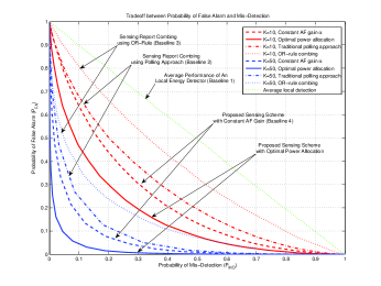
Figure 4: Tradeoff curves between the probability of false alarm and mis-detection. The transmit SNR of the primary user is 30 dB. The mean path loss of the sensing links are $\Lambda_{s}=-30dB$ with variance $\Sigma_{s}=5dB$. The mean path loss of the reporting links are $\Lambda_{r}=-80dB$ with variance $\Sigma_{r}=5dB$. As we can see from the above results, the proposed scheme gives a better tradeoff between the probability of mis-detection and false alarm than other baseline schemes.

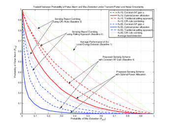
Figure 5: Tradeoff curves between the probability of false alarm and mis-detection under transmit power uncertainties. The mean transmit SNR of the primary user is 30 dB, which is known to all the sensing nodes. The actual transmit SNR of the primary user is frustrated from 30dB to 50dB and the exact value is unknown to all the sensing nodes. The mean path loss of the sensing links are $\Lambda_{s}=-30dB$ with variance $\Sigma_{s}=5dB$. The mean path loss of the reporting links are $\Lambda_{r}=-80dB$ with variance $\Sigma_{r}=5dB$. The noise variances are frustrated from $-5dB$ to $5dB$. As we can see from the above results, under the transmit power uncertainties of the primary systems, the proposed scheme can still work properly and perform better than other baselines.

In this section, we verify our analytical results via simulations. We assume both the noise variance and the channel statistics are assumed to be constant and known at the BS for each static period. Each sensor node has the same channel statistics and experience independent fading. Moreover, each observation chance is chosen to be 2ms and the static period is assumed to be sufficiently long for 10 observation chances. For easy illustration, we define some baseline systems, namely the baseline 1: local detection scheme, the baseline 2: traditional distributed sensing scheme, the baseline 3: OR-Rule combining sensing scheme, and the baseline 4: proposed cooperative sensing scheme with constant AF gain $\alpha$. In baseline 1, we plot the average local detection performance, i.e. the average performance of an energy detector over different sensing positions. In baseline 2, the BS applies polling scheme to each of the sensing node for the sensing report and perform the final decision based on majority voting scheme. In baseline 3, all the sensing node shall report one-bit local decision simultaneously and the BS performs the final decision based on the OR-Rule. For simplicity, we assume perfect reporting links for baselines 2 and 3, i.e. the local decision results of baselines 2 and 3 can be successfully delivered to the BS. On the other hand, for our proposed scheme and baseline 4, the reporting links are modeled by equation (2). Hence, we have more favorable assumptions regarding the reporting links for the baselines. Fig. 4 shows the tradeoff relation between the probability of false alarm $P_{FA}$ and the probability of mis-detection $P_{MD}$. The proposed cooperative sensing scheme performs better than the local detection scheme (baseline 1), the traditional distributed sensing scheme (baseline 2) and the OR-Rule combining sensing schemes (baseline 3) regardless of the power allocation scheme. Meanwhile, the proposed cooperative sensing scheme with optimal power allocation achieves better tradeoff than with constant AF gain scheme (baseline 4). In practise, the actual transmit power of the primary system may difficult to obtain. In Fig. 5, we studies the tradeoff relations when the actual transmit power and the noise variances are unknown to the sensing nodes. Based on the numerical results, we find that the proposed cooperative sensing scheme can still work properly and perform better than other baselines.

Fig. 6 shows the relations between the system performance (i.e. the false alarm and mis-detection error performance) and the number of sensor nodes. Without loss of generality, we choose $\beta$ equals to $1$ and the system performance becomes the sum of the false alarm and mis-detection error probability. As shown in Fig. 6, the system performance of the proposed cooperative sensing scheme with optimal power allocation as well as the constant AF gain allocation scales in the order of $\mathcal{O}\big{(}\exp(-K)\big{)}$ as we have shown in Theorem 2. Fig. 7 and Fig. 8 demonstrate the effects of the reporting links and sensing links. We simulate the number of sensor nodes required to achieve a target probability of false alarm and mis-detection (e.g. we choose $P_{FA}=P_{MD}=0.1$ as specified in IEEE 802.22 [6]) under different qualities of the reporting links and sensing links. As we have shown in the Fig. 7, the number of sensor nodes required is proportional to the qualities of the reporting links $\Sigma_{r}/\rho_{r}^{2}$ as derived in Corollary 1. Fig. 8 illustrates the number of sensor nodes $K$ scales in the order of $\mathcal{O}\big{(}(1+\sqrt{1+\Sigma_{s}})^{2}/\rho_{s}^{2}\big{)}$ w.r.t. the sensing links as derived in Corollary 2.

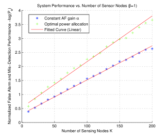
Figure 6: System performance versus number of sensor nodes ($\beta=1$). The simulation points fit very well with the order of growth expression derived. This verifies that the false alarm and mis-detection performance decreases exponentially with respect to the number of sensor nodes $K$ as derived in theorem 2.

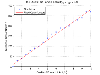
Figure 7: The effect of the reporting links ($P_{FA}=P_{MD}=0.1$). This illustrates the number of sensor nodes required follows $\mathcal{O}(\Sigma_{r}/\rho_{r}^{2})$ as derived in corollary 1.

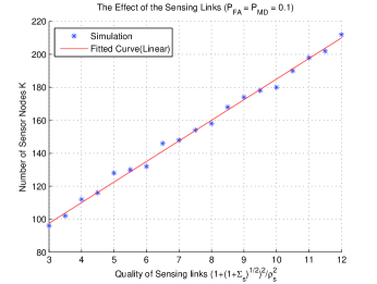
Figure 8: The effect of the sensing links ($P_{FA}=P_{MD}=0.1$). This illustrates the number of sensor nodes required follows $\mathcal{O}\big{(}(1+\sqrt{1+\Sigma_{s}})^{2}/\rho_{s}^{2}\big{)}$ as derived in corollary 2.

VIII Conclusion

In this paper, we proposed a simple cooperative sensing framework for the cognitive radio systems. By applying the proposed cooperative sensing scheme, we formulate the power scheduling algorithm as a multi-objective optimization problem. To describe the relations of the multiple objectives, we characterize the optimal trade-off curve, containing a set of Pareto optimal values for a multi-criteria problem, and derive the asymptotic closed-form expression for the false alarm and mis-detection error performance of the proposed cooperative sensing framework. Simulation results are then evaluated to demonstrate the proposed cooperative sensing framework. We found that the false alarm and mis-detection error performance of the proposed cooperative sensing framework scales in the order of $\mathcal{O}\big{(}\exp(-K)\big{)}$. In order to achieve a target false alarm and mis-detection probability, the number of required sensor nodes scales in the order of $\mathcal{O}\big{(}\Sigma_{r}(1+\sqrt{1+\Sigma_{s}})^{2}/\rho_{r}^{2}\rho_{s}^{2}\big{)}$ in the low SNR regime.

Appendix A Proof of Lemma 1

In order to calculate the probability of mis-detection and false alarm, we shall first try to find the probability density function (p.d.f.) of the received signal $X$ at the BS side. Since the sensing links remain quasi-static throughout the observation chance and the noise variance is completely known at each sensor node, the time average received signal power at the $k^{th}$ sensor node can be expressed as

$$|x_{k}|^{2} = \frac{1}{T}\int_{t=0}^{T}{\big{|}h_{k}^{s}\theta x_{p}\sqrt{P_{pu}}+n_{k,t}^{s}\big{|}}^{2}\textrm{d}t$$ (43)

$$= \frac{1}{T}\Big{(}|h_{k}^{s}\theta x_{p}\sqrt{P_{pu}}|^{2}T+|n_{k}^{s}|^{2}+X_{k}\Big{)}$$

$${\buildrel\text{w.p.1}\over{\longrightarrow}} |h_{k}^{s}|^{2}\theta^{2}P_{pu}+\frac{1}{T}|n_{k}^{s}|^{2}$$

where $n_{k}^{s}$ is the additive white Gaussian noise with mean zero and variance $T$. $X_{k}=2\textrm{Re}\Big{\{}\frac{1}{T}\int_{t=0}^{T}h_{k}^{s}\theta x_{p}\sqrt{P_{pu}}n_{k,t}^{s,*}\textrm{d}t\Big{\}}$ , which is with zero mean and variance $|h_{k}^{s}|^{2}\theta^{2}P_{pu}T$. For sufficiently large $T$, the cross-term $\frac{X_{k}}{T}$ tends to zero with probability 1 (w.p.1). We also assume the noise and primary signals are independent and substitute $|x_{p}|^{2}=1$ in the last step.

At the BS side, the received signal contributed by $k^{th}$ sensor node (denoted by $\hat{\mathcal{X}_{k}}$) is given by

$$\hat{\mathcal{X}_{k}} = h_{k}^{b}\mathcal{X}_{k}=|h_{k}^{r}|^{2}|x_{k}|^{2}\sqrt{\alpha_{k}}$$ (44)

$$= \underbrace{|h_{k}^{r}|^{2}|h_{k}^{s}|^{2}\theta^{2}P_{pu}\sqrt{\alpha_{k}}}_{\textrm{Signal Part}}+\underbrace{\frac{1}{T}|h_{k}^{r}|^{2}|n_{k}^{s}|^{2}\sqrt{\alpha_{k}}}_{\textrm{Noise Part}}$$

The statistical properties of the random variable $\hat{\mathcal{X}_{k}}$ can be evaluated in the following way.

$$\mu_{\hat{\mathcal{X}_{k}}} = \mathbb{E}_{h_{k}^{r},h_{k}^{s},n_{k}^{s}}\big{[}\hat{\mathcal{X}_{k}}\big{]}=\Sigma_{k}^{r}\sqrt{\alpha_{k}}\big{(}\Sigma_{k}^{s}\theta^{2}P_{pu}+1\big{)}$$ (45)

$$\sigma_{\hat{\mathcal{X}_{k}}}^{2} = \mathbb{E}_{h_{k}^{r},h_{k}^{s},n_{k}^{2}}\big{[}(\hat{\mathcal{X}_{k}}-\mu_{\hat{\mathcal{X}_{k}}})^{2}\big{]}$$ (46)

$$= \Sigma_{k}^{r,2}\alpha_{k}(3\Sigma_{k}^{s,2}\theta^{4}P_{pu}^{2}+2\Sigma_{k}^{s}\theta^{2}P_{pu}+3)$$

Using the proposed cooperative sensing scheme, all $K$ sensor nodes are suggested to report their local measurements at the same time and all the reports will naturally combined in the air interface. Applying the central limit theorem [33], the received signal $X$ at the BS side can be approximated by the following equation when $K$ is sufficiently large [12]

$$X\sim\mathcal{N}\bigg{(}\frac{\sum_{k=1}^{K}\mu_{\hat{\mathcal{X}_{k}}}}{K},\frac{\sum_{k=1}^{K}\sigma_{\hat{\mathcal{X}_{k}}}^{2}+1}{K^{2}}\bigg{)}$$ (47)

where $\mathcal{N}(\mu,\sigma^{2})$ denotes the Gaussian distribution with mean $\mu$ and variance $\sigma^{2}$.

Denote $\mu_{1},\sigma_{1}^{2}$ to be the mean and variance of the received signal $X$ when the primary user is in active state and $\mu_{0},\sigma_{0}^{2}$ to be the mean and variance of $X$ when the PU is in idle state, respectively. We can derive the expressions for $\mu_{0},\sigma_{0}^{2},\mu_{1},\sigma_{1}^{2}$ as follows.

$$\mu_{0} = \frac{\sum_{k=1}^{K}\mu_{\hat{\mathcal{X}_{k}}}}{K}=\frac{\sum_{k=1}^{K}\Sigma_{k}^{r}\sqrt{\alpha_{k}}}{K},$$ (48)

$$\sigma_{0}^{2} = \frac{\sum_{k=1}^{K}\sigma_{\hat{\mathcal{X}_{k}}}^{2}}{K^{2}}=\frac{3\sum_{k=1}^{K}{\Sigma_{k}^{r}}^{2}\alpha_{k}+1}{K^{2}}$$ (49)

$$\mu_{1} = \frac{\sum_{k=1}^{K}\mu_{\hat{\mathcal{X}_{k}}}}{K}=\frac{\sum_{k=1}^{K}\Sigma_{k}^{r}\sqrt{\alpha_{k}}(\Sigma_{k}^{s}P_{pu}+1)}{K}$$ (50)

$$\sigma_{1}^{2} = \frac{\sum_{k=1}^{K}\sigma_{\hat{\mathcal{X}_{k}}}^{2}}{K^{2}}$$ (51)

$$= \frac{\sum_{k=1}^{K}{\Sigma_{k}^{r}}^{2}\alpha_{k}(3\Sigma_{k}^{s,2}P_{pu}^{2}+2\Sigma_{k}^{s}P_{pu}+3)+1}{K^{2}}$$

Using these approximations gives the following expressions, we have $Pr\big{(}\hat{\theta}=0|\theta=1,\{\Sigma_{k}^{r},\Sigma_{k}^{s}\},\mathbf{a},\mathcal{T}_{0}\big{)}=1-Q\big{(}\frac{\mathcal{T}_{0}-\mu_{1}}{\sigma_{1}}\big{)}$ and $Pr\big{(}\hat{\theta}=1|\theta=0,\{\Sigma_{k}^{r},\Sigma_{k}^{s}\},\mathbf{a},\mathcal{T}_{0}\big{)}=Q\big{(}\frac{\mathcal{T}_{0}-\mu_{0}}{\sigma_{0}}\big{)}$, where $Q(\cdot)$ denotes the standard Gaussian complementary c.d.f.[29]. Notice that $1-Q(-x)=Q(x)$, we have Lemma 1.

Appendix B Proof of Theorem 1

Since the primal problem (30) is not convex, the standard optimization theory cannot be applied here to prove the zero duality gap. From the result of [31], the primal problem and its dual problem will have zero duality gap when the time-sharing condition is satisfied. The results will hold true even when the primal problem is nonconvex.

Let $P_{1}=\{P_{0,1},P_{1,1},\ldots,P_{K,1}\},P_{2}=\{P_{0,2},P_{1,2},\ldots,P_{K,2}\}$ and $P_{3}=\{P_{0,3},P_{1,3},\ldots,P_{K,3}\}$ be values of power constraints with $P_{3}=\nu P_{1}+(1-\nu)P_{2}$ for some $0\leq\nu\leq 1$. Let $\mathbf{a}_{1}^{*}$, $\mathbf{a}_{2}^{*}$ and $\mathbf{a}_{3}^{*}$ be the optimal power allocation (AF gain) scheme to the primal optimization problem (27) with constraints $P_{1},P_{2}$ and $P_{3}$, respectively. Let $P_{e1}^{*}$ and $P_{e2}^{*}$ be their respective optimal values of the false alarm and mis-detection error performance. To prove the time-sharing property, we need to construct a power allocation (AF gain) scheme $\mathbf{a}_{3}^{*}$ such that it achieves an error equal to or lower than $\nu P_{e1}^{*}+(1-\nu)P_{e2}^{*}$ with a power that is at most $\nu P_{1}+(1-\nu)P_{2}$ for all $\nu$ between zero and one. Such a scheme $\mathbf{a}_{3}^{*}$ may be constructed as follows.

Without loss of generality, we consider the multiple transmission opportunities are divided into two periods with $\nu$ proportion of which corresponding to a power constraint $P_{1}$ and $(1-\nu)$ proportion of which corresponding to a power constraint $P_{2}$. We can apply the power allocation scheme $\mathbf{a}_{1}^{*}$ to the first $\nu$ proportion of channel realizations and $\mathbf{a}_{2}^{*}$ to the rest $(1-\nu)$ proportion. By doing so, the system achieves the value of $(\mathcal{T}_{0}^{*}-\mu_{0})/\sigma_{0}$ at least equal to $\nu P_{e1}^{*}+(1-\nu)P_{e2}^{*}$ and therefore, the time-sharing property holds. From [31, Theorem 1], the primal problem (27) and the dual problem (31) have the same optimal value since the time-sharing condition is satisfied.

Appendix C Proof of Theorem 2

From the expressions of $\mu_{0},\mu_{1},\sigma_{0}^{2}$ and $\sigma_{1}^{2}$, we find that when the number of sensor nodes $K$ is sufficiently large, the following relation holds, $(\mu_{1}-\mu_{0})^{2}\gg 2(\sigma_{1}^{2}-\sigma_{0}^{2})\ln(\beta\sigma_{1}/\sigma_{0})$. Using the above relation, the optimal threshold $\mathcal{T}_{0}^{*}$ from (28) is given by

$$\mathcal{T}_{0}^{*} = \mu_{0}+\frac{\sigma_{0}^{2}(\mu_{0}-\mu_{1})}{\sigma_{1}^{2}-\sigma_{0}^{2}}+\frac{\sigma_{0}\sigma_{1}}{\sigma_{1}^{2}-\sigma_{0}^{2}}$$ (52)

$$\times\sqrt{(\mu_{1}-\mu_{0})^{2}+2(\sigma_{1}^{2}-\sigma_{0}^{2})\ln(\beta\sigma_{1}/\sigma_{0})}$$

$$\approx \mu_{0}+\frac{\sigma_{0}^{2}(\mu_{0}-\mu_{1})+\sigma_{0}\sigma_{1}\sqrt{(\mu_{1}-\mu_{0})^{2}}}{\sigma_{1}^{2}-\sigma_{0}^{2}}$$ (53)

$$= \mu_{0}+\sigma_{0}\frac{\mu_{1}-\mu_{0}}{\sigma_{0}+\sigma_{1}}$$ (54)

Substitute the equation (54) into (41), we have

$$P_{e}^{u}\big{(}\{\Sigma_{k}^{r},\Sigma_{k}^{s}\}\big{)}=(1+\beta)Q(\frac{\mu_{1}-\mu_{0}}{\sigma_{0}+\sigma_{1}})\big{|}_{\mathbf{a}=\alpha\cdot\mathbf{1}}$$ (55)

and the average probability of false alarm and mis-detection is

$$\bar{P}_{e}^{*} \leq \mathbb{E}_{\{\Sigma_{k}^{r},\Sigma_{k}^{s}\}}\Big{[}P_{e}^{u}\big{(}\{\Sigma_{k}^{r},\Sigma_{k}^{s}\}\big{)}\Big{]}$$

$$= \mathbb{E}_{\{\Sigma_{k}^{r},\Sigma_{k}^{s}\}}\Big{[}(1+\beta)Q(\frac{\mu_{1}-\mu_{0}}{\sigma_{0}+\sigma_{1}})\big{|}_{\mathbf{a}=\alpha\cdot\mathbf{1}}\Big{]}$$

$$\leq \mathbb{E}_{\{\Sigma_{k}^{r},\Sigma_{k}^{s}\}}\bigg{[}\frac{1+\beta}{2}\exp\Big{(}-\frac{1}{2}\big{(}\frac{\mu_{1}-\mu_{0}}{\sigma_{0}+\sigma_{1}}\big{)}^{2}\Big{)}\big{|}_{\mathbf{a}=\alpha\cdot\mathbf{1}}\bigg{]}$$

$$\leq \frac{1+\beta}{2}\exp\big{(}-\frac{\gamma^{2}}{2}\big{)}$$ (57)

with $\gamma=\mathbb{E}_{\{\Sigma_{k}^{r},\Sigma_{k}^{s}\}}\bigg{[}\frac{\mu_{1}-\mu_{0}}{\sigma_{0}+\sigma_{1}}\big{|}_{\mathbf{a}=\alpha\cdot\mathbf{1}}\bigg{]}$ where we use the relation $Q(x)\leq\frac{1}{2}\exp(-\frac{x^{2}}{2})$ in the second inequality and the concavity of the function $\exp(-\frac{x^{2}}{2})$ w.r.t. $x$ in the last step.

Applying the statistical model given by (37) to (39), the mean and variance of the received $\textrm{SNR}_{k}^{r}$ and $\textrm{SNR}_{k}^{s}$ under the constant AF gain scheme are given by $(\sqrt{\alpha}\Lambda_{r},\Sigma_{r})$ and $(P_{pu}\Lambda_{s},\Sigma_{s})$, respectively. $\mu_{0},\mu_{1},\sigma_{0}^{2}$ and $\sigma_{1}^{2}$ under the constant AF gain policy $\mathbf{a}=\alpha\cdot\mathbf{1}$ are thus given by

$$\mu_{0} = T\sqrt{\alpha}\Lambda_{r},$$

$$\sigma_{0}^{2} = \frac{3T^{2}(\alpha\Lambda_{r}^{2}+\Sigma_{r})}{K},$$

$$\mu_{1} = T\sqrt{\alpha}\Lambda_{r}(P_{pu}\Lambda_{s}+1),$$

$$\sigma_{1}^{2} = \frac{T^{2}(\alpha\Lambda_{r}^{2}+\Sigma_{r})\big{(}3P_{pu}^{2}\Lambda_{s}^{2}+3\Sigma_{s}+2P_{pu}\Lambda_{s}+3\big{)}}{K}$$

where we have substituted the mean and variance of the received $\textrm{SNR}_{k}^{b}$ and $\textrm{SNR}_{k}^{i}$. Hence, we can evaluate the expression of $\gamma$ as follows.

$$\gamma\approx\sqrt{\frac{K}{3(1+\frac{\Sigma_{r}}{\alpha\Lambda_{r}^{2}})}}\cdot\frac{P_{pu}\Lambda_{s}}{1+\sqrt{P_{pu}^{2}\Lambda_{s}^{2}+\Sigma_{s}+\frac{2P_{pu}\Lambda_{s}}{3}+1}}$$ (58)

Combine (57) and (58), we have Theorem 2.

References

- [1] J. Mitola and G. Q. Maguire, “Cognitive radio: making software radios more personal,” IEEE Personal Commun. Mag., vol. 6, no. 4, pp. 13 – 18, Aug. 1999.
- [2] S. Haykin, “Cognitive radio: brain-empowered wireless communications,” IEEE J. Sel. Areas Commun., vol. 23, no. 2, pp. 201 – 220, Feb. 2005.
- [3] V. K. Bhargava and E. Hossain, Cognitive Wireless communication networks. New York: Springer-Verlag, 2007.
- [4] R. W. Brodersen, A. Wolisz, D. Cabric, S. M. Mishra, and D. Willkomm, CORVUS: a cognitive radio approach for usage of virtual unlicensed spectrum. Berkeley, CA: Univ. California Berkeley, Jul. 2004, white paper.
- [5] FCC 04-113, FCC, May 2004. [Online]. Available: http://hraunfoss.fcc.gov/edocs_public/attachmatch/FCC-04-113A1.pdf
- [6] IEEE 802.22/D0.1, Draft Standard for Wireless Regional Area Networks Part22: Cognitive Wireless RAN Medium Access Control (MAC) and Physical Layer (PHY) specifications: Policies and procedures for operation in the TV Bands, IEEE standard, IEEE, May 2006.
- [7] V. R. Cadambe and S. A. Jafar, “Interference alignment and the degrees of freedom for the K user interference channel,” IEEE Trans. Inf. Theory, 2007, to be published.
- [8] N. Devroye, P. Mitran, and V. Tarokh, “Achievable rates in cognitive radio channels,” IEEE Trans. Inf. Theory, vol. 52, no. 5, pp. 1813 – 1827, May 2006.
- [9] X. H. C. Wang, H. H. Chen, and J. Thompson, “Performance analysis of cognitive radio networks with average interference power constraints,” in Proc. of Communications, IEEE International Conference on, 2008, May 2008, pp. 3578 – 3582.
- [10] K. Hamdi, W. Zhang, and K. B. Letaief, “Uplink scheduling with qos provisioning for cognitive radio systems,” in Proc. of IEEE Wireless Communications and Networking Conference, 2007, Mar. 2007, pp. 2592 – 2596.
- [11] A. Sahai, N. Hoven, and R. Tandra, “Some fundamental limits on cognitive radio,” in Proc. of 42nd Allerton Conf. Communications, Control and Computing, Monticello, IL, Oct. 2004.
- [12] R. Tandra and A. Sahai, “SNR Walls for Signal Detection,” IEEE J. Sel. Areas Commun., vol. 2, no. 1, pp. 4 – 17, Feb. 2008.
- [13] S. M. Kay, Fundamentals of statistical signal processing: detection theory, 2nd ed. Englewood Cliffs: Prentice-Hall, 1998, vol. 2.
- [14] H. V. Poor, An introduction to signal detection and estimation, 2nd ed. New York: Springer, Mar. 1998.
- [15] J. Unnikrishnan and V. V. Veeravalli, “Cooperative sensing for primary detection in cognitive radio,” IEEE J. Sel. Areas Signal Process., vol. 2, no. 1, pp. 18 – 27, Feb. 2008.
- [16] E. Visotsky, S. Kuffner, and R. Peterson, “On collaborative detection of TV transmissions in support of dynamic spectrum sharing,” in Proc. of 1st IEEE Int. Symp. New Frontiers in Dynamic Spectrum Access Networks, 2005, pp. 338 – 345.
- [17] S. M. Mishra, A. Sahai, and R. W. Brodersen, “Cooperative sensing among cognitive radios,” in Proc. of 1st IEEE Int. Conf. Communications, vol. 4, 2006, pp. 1658 – 1663.
- [18] A. Anandkumar and L. Tong, “Type-based random access for distributed detection over multiaccess fading channels,” IEEE Trans. Signal Process., vol. 55, no. 10, pp. 5032 – 5043, Oct. 2007.
- [19] K. Liu and A. M. Sayeed, “Type-based decentralized detection in wireless sensor networks,” IEEE Trans. Signal Process., vol. 55, no. 5, pp. 1899 – 1910, May 2007.
- [20] C. Sun, W. Zhang, and K. B. Letaief, “Cooperative spectrum sensing for cognitive radios under bandwidth constraints,” in Proceedings of IEEE Wireless Communications and Networking Conference (WCNC), Hong Kong, Mar. 2007, pp. 1 – 5.
- [21] J. Lunden, V. Koivunen, A. Huttunen, and H. V. Poor, “Censoring for collaborative spectrum sensing in cognitive radios,” in Conference Record of the Forty-First Asilomar Conference on Signals, Systems, and Computers, Pacific Grove, CA, Nov. 2007, pp. 772 – 776.
- [22] S. Chaudhari, V. Koivunen, and H. V. Poor, “Distributed autocorrelation-based sequential detection of ofdm signals in cognitive radios,” in 3rd International Conference on Cognitive Radio Oriented Wireless Networks and Communications (CrownCom), Singapore, May 2008, pp. 1 – 6.
- [23] A. Taherpour, Y. Norouzi, M. Nasiri-Kenari, A. Jamshidi, and Z. Zeinalpour-Yazdi, “Asymptotically optimum detection of primary user in cognitive radio networks,” IET Communications, vol. 1, no. 6, pp. 1138 – 1145, Dec. 2007.
- [24] E. Peh and Y.-C. Liang, “Optimization for cooperative sensing in cognitive radio networks,” in Proceedings of IEEE Wireless Communications and Networking Conference (WCNC), Hong Kong, Mar. 2005, pp. 27 – 32.
- [25] Y.-C. Liang, Y. Zeng, E. C. Peh, and A. T. Hoang, “Sensing-throughput tradeoff for cognitive radio networks,” IEEE Trans. Wireless Commun., vol. 7, no. 4, pp. 1326 – 1337, Apr. 2008.
- [26] B. Chen, R. Jiang, T. Kasetkasem, and P. K. Varshney, “Channel aware decision fusion in wireless sensor networks,” IEEE Trans. Signal Process., vol. 52, no. 12, pp. 3454 – 3458, Dec. 2004.
- [27] R. Jiang and B. Chen, “Fusion of censored decisions in wireless sensor networks,” IEEE Trans. Wireless Commun., vol. 4, no. 6, pp. 2668 – 2673, Nov. 2005.
- [28] Z. Quan, S. Cui, and A. H. Sayed, “Optimal linear cooperation for spectrum sensing in cognitive radio networks,” IEEE J. Sel. Areas Signal Process., vol. 2, no. 1, pp. 28 – 40, Feb. 2008.
- [29] J. G. Proakis, Digital Communication. McGraw-Hill, 2000.
- [30] S. Boyd and L. Vandenberghe, Convex Optimization. Cambridge University Press, 2003.
- [31] W. Yu and R. Lui, “Dual methods for nonconvex spectrum optimization of multicarrier systems,” IEEE Trans. Commun., vol. 54, no. 7, pp. 1310 – 1322, Jul. 2006.
- [32] Y. Zeng and Y. C. Liang, “Spectrum-sensing algorithms for cognitive radio based on statistical covariances,” IEEE Trans. Veh. Technol., vol. 58, no. 4, pp. 1804 – 1815, May 2009.
- [33] A. Papoulis and S. U. Pillai, Probability, Random Variables and Stochastic Processes, 4th ed. McGraw-Hill Companies, Inc., 2002.