The $\alpha$ effect in rotating convection with sinusoidal shear

Abstract

Using three-dimensional convection simulations it is shown that a sinusoidal variation of horizontal shear leads to a kinematic $\alpha$ effect with a similar sinusoidal variation. The effect exists even for weak stratification and arises owing to the inhomogeneity of turbulence and the presence of impenetrable vertical boundaries. This system produces large-scale magnetic fields that also show a sinusoidal variation in the cross-stream direction. It is argued that earlier investigations overlooked these phenomena partly because of the use of horizontal averaging and also because measurements of $\alpha$ using an imposed field combined with long time averages give erroneous results. It is demonstrated that in such cases the actual horizontally averaged mean field becomes non-uniform. The turbulent magnetic diffusion term resulting from such non-uniform fields can then no longer be neglected and begins to balance the $\alpha$ effect.

1 Introduction

Shear can play an important role in hydromagnetic dynamos. This is especially true of dynamos in astrophysical bodies that generate magnetic fields on scales larger than the scale of the turbulent motions. Those types of dynamos are generally referred to as large-scale dynamos. Simulations confirm that shear can be the sole driver of dynamo action (Brandenburg, 2005; Yousef et al., 2008a, b; Brandenburg et al., 2008a), but there is no consensus as to what is the underlying mechanism for producing such large-scale fields. In addition to shear there are also other possible mechanisms producing large-scale magnetic fields. One important contender is the $\alpha$ effect (Steenbeck et al., 1966), which quantifies the effect of kinetic helicity on magnetic field generation. It can also be the sole driver of large-scale dynamo action (Brandenburg, 2001; Käpylä et al., 2009b).

When both shear and $\alpha$ effect act simultaneously, it becomes even harder to identify the main drivers of large-scale dynamo action. Although shear is generally believed to be advantageous for large-scale dynamo action (e.g. Tobias, 2009), it is conceivable that the two effects ($\alpha$ effect and shear) suppress each other at least partially. This is because, in the presence of stratification or other inhomogeneities, shear itself can produce an $\alpha$ effect (Rogachevskii & Kleeorin, 2003; Rädler & Stepanov, 2006; Käpylä et al., 2009a). Its sign depends on the relative orientation of shear and stratification. The net $\alpha$ depends then on the pseudo scalar $(2\bm{\Omega}+\overline{\bm{W}})\cdot\bm{g}$, where $2\bm{\Omega}$ and $\overline{\bm{W}}$ are the vorticities associated with rotation and large-scale shear flow, respectively.

The issue can be complicated even further if shear is not constant but has a sinusoidal profile, for example (Brandenburg et al., 2001; Hughes & Proctor, 2009). Sinusoidal shear profiles are commonly adopted in numerical simulations where all boundaries are strictly periodic. This has obvious computational advantages and is certainly easier to implement than the so-called shearing-periodic boundary conditions where cross-stream periodicity applies only to positions that follow the shear flow and are thus changing with time (Wisdom & Tremaine, 1988). In helical turbulence with shear there is the possibility of dynamo waves that propagate perpendicular to the plane of the shear. This is clearly borne out by simulations (Käpylä & Brandenburg, 2009). The propagation direction of the dynamo wave is proportional to the product $H_{\rm K}\overline{\bm{W}}$, where $H_{\rm K}$ is the kinetic helicity of the flow. When the shear is sinusoidal, the sign of $\overline{\bm{W}}$ changes in space, so one obtains counter-propagating dynamo waves in the two halves of the domain (Brandenburg et al., 2001). In the presence of helicity, there is also a turbulent pumping effect, whose effective velocity is also in the direction of $H_{\rm K}\overline{\bm{W}}$ (Mitra et al., 2009).

In the cases discussed above the turbulence is driven by a helical body force, which is clearly artificial, but it allows contact to be made with analytic theories of dynamo action in homogeneous media (Moffatt, 1978). A more realistic case is one where the turbulence is driven by natural convection in a slab with a temperature gradient in the vertical direction. Many of the features of dynamo action discussed above carry over to this case as well, but an additional complication arises both from the fact that there are impenetrable walls and that the sign of kinetic helicity changes with depth (e.g. Brandenburg et al., 1990; Cattaneo & Hughes, 2006).

In the present paper we deal with both aspects, but we focus in particular on the effects of sinusoidal shear, where we expect at least partial cancellation of the $\alpha$ effect when averaged over horizontal planes. We contrast our work with earlier results that used linear shear, implemented via the shearing-box approximation (Käpylä et al., 2008), as well as the case with no shear (Käpylä et al., 2009b), where only the $\alpha$ effect can operate. The conclusion from these studies is that in the simulation domain there is an $\alpha$ effect of the strength expected from kinematic mean-field theory (Käpylä et al., 2009a, b). There is also a back-reaction of the magnetic field through the Lorentz force, and its strength varies depending on whether or not magnetic helicity is allowed to escape from the domain (Käpylä et al., 2009c). Again, these aspects are now well understood using mean-field theory. The new aspect here is the sinusoidal shear. In a recent paper, Hughes & Proctor (2009) present results from convection simulations with rotation and large-scale shear and report the emergence of a large-scale magnetic field whose growth rate is proportional to the shear rate, similar to the earlier results of Käpylä et al. (2008). They also determine the $\alpha$ effect from their simulations using the so-called imposed-field method and find that $\alpha$ is small and unaffected by the presence of shear. From these results the authors conclude that the dynamo cannot be explained by a classical $\alpha^{2}$ or $\alpha\Omega$ dynamo.

The interpretation of the results of Hughes & Proctor (2009) is potentially in conflict with that of Käpylä et al. (2008). In both cases, convection together with shear was found to produce large-scale fields, but in Käpylä et al. (2008) they are interpreted as being the result of a conventional $\alpha$ effect while in Hughes & Proctor (2009) it is argued that they are due to another mechanism similar to the incoherent $\alpha$–shear effect (Vishniac & Brandenburg, 1997; Sokolov, 1997; Silant’ev, 2000; Proctor, 2007), or perhaps the shear–current effect (Rogachevskii & Kleeorin, 2003, 2004). Moreover, Hughes & Proctor (2009) argue that the $\alpha$ effect is ruled out.

At this point we cannot be sure that there is really a difference in interpretations, because the systems considered by Käpylä et al. (2008) and Hughes & Proctor (2009) are different in at least two important aspects. Firstly, in Hughes & Proctor (2009) there is no density stratification, and since $\alpha$ is supposed to be proportional to the logarithmic density gradient (Steenbeck et al., 1966) the resulting $\alpha$ may indeed vanish. However, due to the impenetrable vertical boundaries, the turbulence is inhomogeneous so that $\bm{\nabla}\ln u_{\rm rms}\neq{\bm{0}}$, which can also lead to an $\alpha$ effect (e.g. Giesecke et al., 2005). Here, $u_{\rm rms}$ is the rms velocity of the turbulence. Secondly, the shear profile changes sign in the horizontal direction. Together with the vertical inhomogeneity this also produces an $\alpha$ effect (Rogachevskii & Kleeorin, 2003; Rädler & Stepanov, 2006), but its contribution is not captured by horizontal averaging and it partially cancels the $\alpha$ effect from rotation. This should be a measurable effect which was not quantified in Hughes & Proctor (2009). Doing this is one of the main motivations behind our present paper.

There is yet another important issue relevant to determining $\alpha$ in a system where the magnetic Reynolds number is large enough to result in dynamo action (Hubbard et al., 2009). Obviously, any successful $\alpha$ effect should produce large-scale magnetic fields. Given enough time, this field should reach saturation. By employing a weak external field one might therefore measure $\alpha$ at a saturated level. Depending on boundary conditions, which were unfortunately not specified in Hughes & Proctor (2009), the saturation can result in a catastrophically quenched $\alpha$ effect. Furthermore, here we show that even in the absence of a dynamo the electromotive force from long time averages reflects not only $\alpha$ due to the uniform imposed field as assumed by Hughes & Proctor (2009), but also picks up contributions from the additionally generated nonuniform fields of comparable magnitude. These caveats in determining $\alpha$ with an externally imposed field were known for some time (Ossendrijver et al., 2002; Käpylä et al., 2006), but they have only recently been examined in detail (Hubbard et al., 2009) and were therefore not addressed by Hughes & Proctor (2009). This gives another motivation to our study.

Here we use a similar simulation setup as Hughes & Proctor (2009) and derive the $\alpha$ effect with the imposed-field method. We show that the value of $\alpha$ determined by the method of resetting the magnetic field after regular time intervals yields a substantially higher value than that reported by Hughes & Proctor (2009). Furthermore, we show that for a sinusoidally varying shear, also the $\alpha$ effect will have a sinusoidal variation in the horizontal direction, hence explaining why Hughes & Proctor (2009) did not see the contribution of shear in their horizontally averaged results.

2 The model

In an effort to compare with the study of Hughes & Proctor (2009), we use a Cartesian domain with $L_{x}=L_{y}=5d$ and $L_{z}=d$ with $0<z<d$, where $d$ is the depth of the convectively unstable layer. We solve the usual set of hydromagnetic equations

$$\frac{\partial\bm{A}}{\partial t} = \bm{U}\times\bm{B}-\eta\mu_{0}\bm{J},$$ (1)

$$\frac{D\ln\rho}{Dt} = -\bm{\nabla}\cdot\bm{U},$$ (2)

$$\frac{D\bm{U}}{Dt} = -\frac{1}{\rho}{\bm{\nabla}}p+{\bm{g}}-2\,\bm{\Omega}\times\bm{U}+\frac{1}{\rho}\bm{J}\times{\bm{B}}$$ (3)

$$\hskip 42.67912pt+\frac{1}{\rho}\bm{\nabla}\cdot 2\nu\rho\mbox{\boldmath${\sf S}$}+\frac{1}{\tau}(\bm{U}-\overline{\bm{U}}^{(0)}),$$

$$\frac{De}{Dt}\! = \!-\frac{p}{\rho}\bm{\nabla}\cdot{\bm{U}}+\frac{1}{\rho}\bm{\nabla}\cdot K\bm{\nabla}T+2\nu\mbox{\boldmath${\sf S}$}^{2}+\frac{\mu_{0}\eta}{\rho}\bm{J}^{2},$$ (4)

where $D/Dt=\partial/\partial t+\bm{U}\cdot\bm{\nabla}$ is the advective time derivative, $\bm{A}$ is the magnetic vector potential, $\bm{B}=\bm{\nabla}\times\bm{A}$ the magnetic field, and $\bm{J}=\mu_{0}^{-1}\bm{\nabla}\times\bm{B}$ is the current density, $\mu_{0}$ is the vacuum permeability, $\eta$ and $\nu$ are the magnetic diffusivity and kinematic viscosity, respectively, $K$ is the heat conductivity, $\rho$ is the density, $\bm{U}$ is the velocity, $\bm{g}=-g\hat{\bm{z}}$ the gravitational acceleration, and $\bm{\Omega}=\Omega_{0}(0,0,1)$ the rotation vector. The fluid obeys an ideal gas law $p=\rho e(\gamma-1)$, where $p$ and $e$ are the pressure and internal energy, respectively, and $\gamma=c_{\rm P}/c_{\rm V}=5/3$ is the ratio of specific heats at constant pressure and volume, respectively. The specific internal energy per unit mass is related to the temperature via $e=c_{\rm V}T$. The rate of strain tensor ${\sf S}$ is given by

$${\sf S}_{ij}={\textstyle{1\over 2}}(U_{i,j}+U_{j,i})-{\textstyle{1\over 3}}\delta_{ij}\bm{\nabla}\cdot\bm{U}.$$ (5)

The last term of equation (3) maintains a shear flow of the form

$$\overline{\bm{U}}^{(0)}=U_{0}\cos\left[\frac{2\pi(x-x_{0})}{L_{x}}\right]\hat{\bm{e}}_{y},$$ (6)

where $U_{0}$ is the amplitude of the shear flow, $x_{0}=-L_{x}/2$ is the position of the left-hand boundary of the domain, and $\tau$ is a relaxation time. Here we use a $\tau=20\sqrt{d/g}$ which corresponds to roughly 3.5 convective turnover times.

In their study, Hughes & Proctor (2009) use the Boussinesq approximation and thus neglect density stratification. Here we use the Pencil Code which is fully compressible. However, in order to stay close to the setup of Hughes & Proctor (2009) we employ a weak stratification: the density difference between the top and the bottom of the domain is only ten per cent and the average Mach number is always less than 0.1. Hence the effects of compressibility are small. The stratification in the associated hydrostatic initial state can be described by a polytrope with index $m=1$. Unlike our previous studies (e.g. Käpylä et al., 2008), no stably stratified layers are present.

The horizontal boundaries are periodic. We keep the temperature fixed at the top and bottom boundaries. For the velocity we apply impenetrable, stress-free conditions according to

$$\partial_{z}U_{x}=\partial_{z}U_{y}=U_{z}=0.$$ (7)

For the magnetic field we use vertical field conditions

$$B_{x}=B_{y}=0,$$ (8)

that allow magnetic helicity to escape from the domain.

Table 1: Summary of the runs. Here ${\rm Ma}=U_{\rm rms}/\sqrt{dg}$, where $U_{\rm rms}$ is the total rms velocity including the shear flow, ${\rm Ma}_{0}=u_{\rm rms}/\sqrt{dg}$, and $\tilde{B}_{\rm rms}=B_{\rm rms}/B_{\rm eq}$, where $B_{\rm eq}=\sqrt{\mu_{0}\rho u_{\rm rms}^{2}}$. We use ${\rm Rm}\approx 18$, ${\rm Co}\approx 2.3$, and ${\rm Ra}=10^{5}$ in all runs.

Run $\rm Ma$ ${\rm Ma}/{\rm Ma_{0}}$ ${\rm Sh}$ $\tilde{B}_{\rm rms}$ Dynamo A0 $0.028$ $1.00$ $0.00$ – no A1 $0.027$ $0.98$ $0.07$ – no A2 $0.028$ $1.01$ $0.14$ $0.70$ yes A3 $0.039$ $1.42$ $0.36$ $1.15$ yes A4 $0.063$ $2.28$ $0.72$ $1.97$ yes A5 $0.096$ $3.47$ $1.45$ $3.99$ yes

2.1 Units, nondimensional quantities, and parameters

Dimensionless quantities are obtained by setting

$$d=g=\rho_{0}=c_{\rm P}=\mu_{0}=1\;,$$ (9)

where $\rho_{0}$ is the density at $z_{\rm m}={\textstyle{1\over 2}}d$. The units of length, time, velocity, density, specific entropy, and magnetic field are then

$$[x]=d\;,\;\;[t]=\sqrt{d/g}\;,\;\;[U]=\sqrt{dg}\;,\;\;$$

$$[\rho]=\rho_{0}\;,\;\;[s]=c_{\rm P}\;,\;\;[B]=\sqrt{dg\rho_{0}\mu_{0}}\;.$$ (10)

The simulations are controlled by the following dimensionless parameters: thermal and magnetic diffusion in comparison to viscosity are measured by the Prandtl numbers

$$\Pr=\frac{\nu}{\chi_{0}},\quad{\rm Pm}=\frac{\nu}{\eta},$$ (11)

where $\chi_{0}=K/(c_{\rm P}\rho_{0})$ is the reference value of the thermal diffusion coefficient, measured in the middle of the layer, $z_{\rm m}$, in the non-convecting initial state. We use $\Pr=0.6$ and ${\rm Pm}=2$ in most models. Note that Hughes & Proctor (2009) use $\Pr=1$ and ${\rm Pm}=5$, but based on earlier parameter studies (Käpylä et al., 2009a, c) we do not expect this difference to be significant. The efficiency of convection is measured by the Rayleigh number

$${\rm Ra}=\frac{gd^{4}}{\nu\chi_{0}}\left(-\frac{1}{c_{\rm P}}\frac{{\rm d}s}{{\rm d}z}\right)_{z_{\rm m}},$$ (12)

again determined from the initial non-convecting state at $z_{\rm m}$. The entropy gradient can be presented in terms of logarithmic temperature gradients

$$\left(-\frac{1}{c_{\rm P}}\frac{{\rm d}s}{{\rm d}z}\right)_{z_{\rm m}}=\frac{\nabla-\nabla_{\rm ad}}{H_{\rm P}},$$ (13)

with $\nabla=(\partial\ln T/\partial\ln p)_{z_{\rm m}}$, $\nabla_{\rm ad}=1-1/\gamma$, and $H_{\rm P}$ being the pressure scale height at $z=z_{\rm m}$.

The effects of viscosity and magnetic diffusion are quantified respectively by the fluid and magnetic Reynolds numbers

$${\rm Re}=\frac{u_{\rm rms}}{\nu k_{\rm f}},\quad{\rm Rm}=\frac{u_{\rm rms}}{\eta k_{\rm f}}={\rm Pm}\,{\rm Re},$$ (14)

where $u_{\rm rms}$ is the root-mean-square (rms) value of the velocity taken from a run where $\overline{\bm{U}}^{(0)}={\bm{0}}$, and $k_{\rm f}=2\pi/d$ is the wavenumber corresponding to the depth of the convectively unstable layer. The strengths of rotation and shear are measured by the Coriolis and shear numbers

$${\rm Co}=\frac{2\Omega}{u_{\rm rms}k_{\rm f}},\quad{\rm Sh}=\frac{S}{u_{\rm rms}k_{\rm f}},$$ (15)

where $S=2\pi U_{0}/L_{x}$.

The size of error bars is estimated by dividing the time series into three equally long parts. The largest deviation of the average for each of the three parts from that over the full time series is taken to represent the error.

Figure 1: Root mean square value of the total magnetic field as a function of time for the runs listed in Table 1.

3 Results

3.1 Dynamo excitation

We first set out to reproduce the results of Hughes & Proctor (2009). To achieve this, we take a run with parameters close to theirs which does not act as a dynamo in the absence of shear (${\rm Sh}=0$). For this baseline simulation we choose the parameters ${\rm Rm}\approx 18$ and ${\rm Co}\approx 2.3$. We then follow the same procedure as Hughes & Proctor (2009) and gradually increase ${\rm Sh}$ whilst keeping all other parameters constant (Table 1) and determine the growth rate $\lambda$ of the magnetic field.

The time evolution of the rms-value of the total magnetic field from our set of runs is presented in Fig. 1. We find no dynamo for ${\rm Sh}=0$ and for weak shear with ${\rm Sh}=0.07$, the growth rate of the field remains virtually the same as in the absence of shear. This can be understood as follows: imposing large-scale shear via a relaxation term effectively introduces a friction term for $U_{y}$ in places where $\bm{U}-\overline{\bm{U}}^{(0)}\neq\bm{0}$, hence lowering the Reynolds number somewhat. However, as the same relaxation time $\tau u_{\rm rms}k_{\rm f}\approx 3.5$ is used in all runs with shear, we are confident that these runs can be compared with each other. As the shear is increased beyond ${\rm Sh}=0.07$, the growth rate first increases roughly directly proportional to the shear rate $S$ (Fig. 2). However, for ${\rm Sh}>0.72$ the increase of the growth rate slows down similarly as in several previous studies (Yousef et al., 2008b; Käpylä et al., 2008; Hughes & Proctor, 2009).

Figure 2: Growth rate $\lambda$ of the total magnetic field, divided by the shear rate $S$ as a function of ${\rm Sh}$.

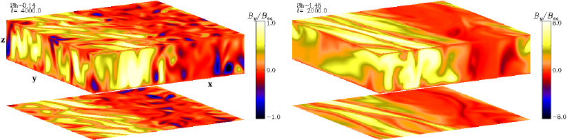
Figure 3: Magnetic field component $B_{y}$ in the saturated state from two runs with weak (left panel, ${\rm Sh}\approx 0.14$, $tu_{\rm rms}k_{\rm f}\approx 700$) and strong shear (right panel, ${\rm Sh}\approx 1.45$, $tu_{\rm rms}k_{\rm f}\approx 350$). The sides of the boxes show the field at the periphery of the domain whereas the bottom (top) panel depicts $B_{y}$ from $z=0.05d$ ($z=0.95d$).

3.2 Field structure

In earlier studies where a homogeneous shear flow was used, the large-scale magnetic field in the saturated state was non-oscillating, showed little dependence on horizontal coordinates, and could hence be well represented by a horizontal average (Käpylä et al., 2008). However, in the present case with sinusoidal shear, the field structure and temporal behaviour can in principle be more complicated. Furthermore, Hughes & Proctor (2009) do not comment on the field structure in their study. In fact, the only evidence of a large-scale field in their paper is given in the form of spectra of the magnetic field.

We find that in our simulations the large-scale field is non-oscillating. It turns out that the magnetic field shows an interesting spatial dependence. In Fig. 3 we show visualizations of the structure of the $B_{y}$ component from the runs with the weakest (${\rm Sh}\approx 0.14$) and the strongest (${\rm Sh}\approx 1.45$) shear in which dynamo action was detected. In both cases it is clear that the strong large-scale fields are concentrated to one side of the computational domain whereas the other side of the box is almost devoid of strong coherent fields. This behaviour is even more striking when the field is averaged over $y$ and $t$; see Fig. 4. In the next section we show that the region of strong large-scale fields coincides with the region where the $\alpha$ effect is strongest.

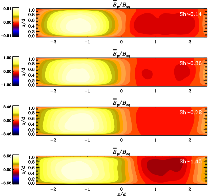
Figure 4: Magnetic field component $B_{y}$ averaged over the saturated state in time and over the $y$-dimension from Runs A2-A5.

3.3 $\alpha$ effect

The origin of large-scale magnetic fields in helical turbulence is commonly attributed to the $\alpha$ effect in turbulent dynamo theory (e.g. Moffatt, 1978; Krause & Rädler, 1980; Rüdiger & Hollerbach, 2004). Results for convection simulations, making use of the test-field method (Käpylä et al., 2009b), suggest that the $\alpha$ effect does indeed contribute to large-scale dynamo action in simulations presented by Käpylä et al. (2008). However, it was also shown that, in order to fully explain the simulation results, additional contributions from the shear–current and $\overline{\bm{\Omega}}\times\overline{\bm{J}}$ effects (Rädler, 1969) appear to be needed.

On the other hand, Hughes & Proctor (2009) claim that in their setup the $\alpha$ effect is small, unaffected by shear, and thus incapable of driving a large-scale dynamo. The setup of Hughes & Proctor (2009) is based on the Boussinesq approximation whereby stratification is not present in their system. However, the impenetrable vertical boundaries also generate an inhomogeneity, which, in a rotating system leads to an $\alpha$ effect of the form (Steenbeck et al., 1966)

$$\alpha_{ij}^{(\Omega)}=\alpha_{1}(\bm{G}\cdot\bm{\Omega})\delta_{ij}+\alpha_{2}(G_{i}\Omega_{j}+G_{j}\Omega_{i}),$$ (16)

where $G_{i}$ denotes the inhomogeneity and $\bm{\Omega}$ is the rotation vector. In Boussinesq convection with rotation the kinetic helicity and thus the $\alpha$ effect are antisymmetric around the midplane of the layer. In such cases it can be useful to average over one vertical half of the layer to obtain an estimate of $\alpha$. We note that mean-field dynamo models have shown that the details of the $\alpha$ profile can also play a significant role (e.g. Baryshnikova & Shukurov, 1987; Stefani & Gerbeth, 2003). In what follows, we show in most cases the full profile of $\alpha$ and present averages over the upper half of the domain only when comparing directly to Hughes & Proctor (2009). Since the simulations in the present paper are weakly stratified, only minor deviations from a perfectly symmetric profile can be expected to occur.

Adding a shear flow of the form presented in equation (6) produces large-scale vorticity $\overline{W}_{z}\propto\sin\tilde{x}$, where $\tilde{x}$ is a shifted and rescaled $x$ coordinate with $\tilde{x}=2\pi(x-x_{0})/L_{x}$. Such vorticity leads to an $\alpha$ effect (see, e.g. Rogachevskii & Kleeorin, 2003; Rädler & Stepanov, 2006),

$$\alpha_{ij}^{(\overline{\bm{W}})}=\alpha_{1}(\bm{G}\cdot\overline{\bm{W}})\delta_{ij}+\alpha_{2}(G_{i}\overline{W}_{j}+G_{j}\overline{W}_{i}),$$ (17)

which, in the present case, leads to $\alpha_{yy}\propto\sin\tilde{x}$. Thus, when both rotation and shear are present, $\alpha=\alpha(x,z)$ is a function of both $x$ and $z$.

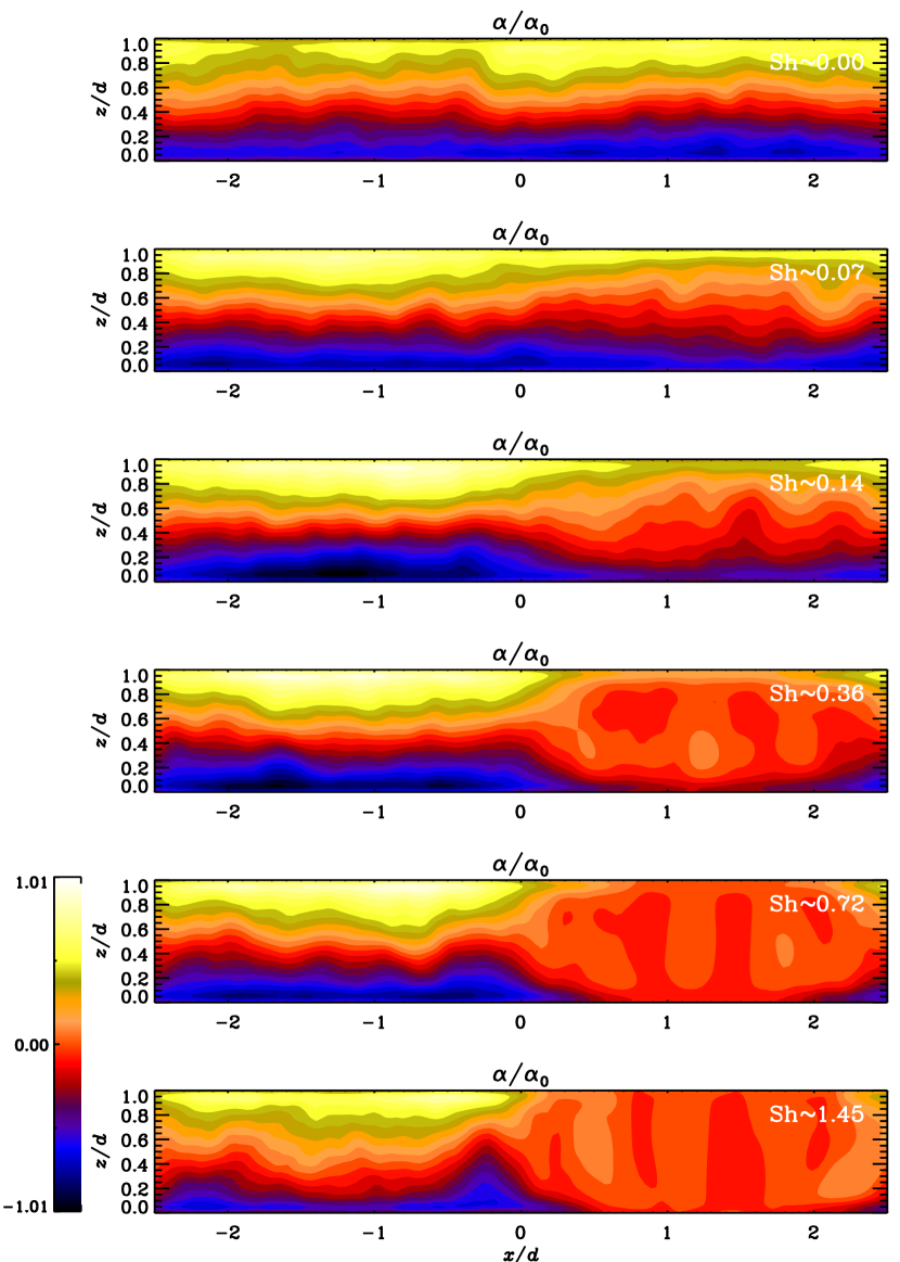
Figure 5: The coefficient $\alpha$, averaged over the $y$-direction and time for Runs A0-A5.

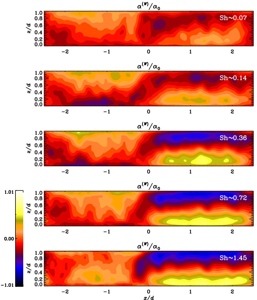
Figure 6: The contribution of shear to the $\alpha$ effect according to equation (21), averaged over the $y$-coordinate and time for Runs A1-A5.

In order to measure the $\alpha$ effect, we impose a weak uniform magnetic field $B_{0}\hat{\bm{e}}_{y}$, with $B_{0}\approx 4\cdot 10^{-5}B_{\rm eq}$, and measure the response of the relevant ($y$) component of the electromotive force. Our $\alpha$ is then obtained from

$$\alpha\equiv\alpha_{yy}=\mathcal{\overline{E}}_{y}/B_{0}.$$ (18)

In contrast to the study of Hughes & Proctor (2009), we do not usually allow the field that is generated in addition to $B_{0}$ to saturate, but reset it after a time interval $\Delta t\approx 10\ tu_{\rm rms}k_{\rm f}$. Such a procedure was first introduced by Ossendrijver et al. (2002) and it was used also in Käpylä et al. (2006) to circumvent the complications that arise due to the additionally generated fields. A more systematic study of Hubbard et al. (2009) showed that only if $\Delta t$ is not too long, the kinematic value of $\alpha$ can be obtained if there is a successful large-scale dynamo present in the system. However, in the present study and also in that of Hughes & Proctor (2009) there is no dynamo in the runs from which $\alpha$ is computed. We find that it is still necessary to use resetting to obtain the correct value of $\alpha$ even in the absence of a dynamo. However, we postpone detailed discussion of this issue to Section 3.4.

Figure 7: The coefficient $\alpha$ averaged over the upper half ($0.5d<z<d$) of the domain from the left ($x<0$, solid line) and right ($x>0$, dashed line) sides of the box.

Our results for $\alpha$ from runs with constant rotation and varying shear are shown in Fig. 5. We find that in the absence of shear, $\alpha$ is a function only of $z$ and has a magnitude of about $0.6\alpha_{0}$, where $\alpha_{0}={\textstyle{1\over 3}}u_{\rm rms}$ is a reference value, and $u_{\rm rms}$ is taken from a run with ${\rm Sh}=0$. When shear is introduced, $\alpha$ increases (decreases) in the regions of the domain where $\sin\tilde{x}>0$ ($\sin\tilde{x}<0$). However, for strong shear, the contribution to $\alpha$ from shear no longer appears to be symmetric around $x=0$. This can be understood in terms of the shear parameter

$$q=-\frac{\partial\overline{U}^{(0)}}{\partial x}/\Omega,$$ (19)

where

$$\frac{\partial\overline{U}^{(0)}}{\partial x}=S\sin\tilde{x}.$$ (20)

The flow is linearly unstable for $q>2$ (Rayleigh instability criterion). Although the maximum value of $q$ in our simulations is about $1.25$ it is clear that for ${\rm Sh}\ga 0.36$ (with $|q|\ga 0.31$), the profile and the magnitude of $\alpha$ are no longer significantly affected by the increasing shear. In order to illustrate this we compute the contribution of $\alpha$ due to shear from runs with ${\rm Sh}\neq 0$ by subtracting the $\alpha$ that was found in the absence of shear using

$$\alpha^{(\overline{W})}=\alpha-\alpha^{(\Omega)},$$ (21)

where $\alpha^{(\Omega)}$ is the $\alpha$ obtained from Run A0 with no shear but only rotation. The results are shown in Fig. 6 and clearly show that for small ${\rm Sh}$ ($\la 0.14$), the shear-induced $\alpha$ shows a sinusoidal variation as a function of $x$. For larger shear the profile of $\alpha^{(\overline{W})}$ is no longer antisymmetric around $x=0$. This could reflect the asymmetry of the results for $q>0$ ($-L_{x}/2<x<0$) and $q<0$ ($0<x<L_{x}/2$), that was found earlier by Snellman et al. (2009) in a somewhat different context of forced turbulence under the influence of rotation and shear. They found that the Reynolds stresses were significantly different in setups with different sign of ${\rm Sh}$ or $q$, and that this asymmetry became more pronounced when the magnitude of shear was increased. Similar behavior has been seen in the magnetohydrodynamic regime by Korpi et al. (2009) in the Reynolds and Maxwell stresses.

We also observe that the magnitude of $\alpha^{(\overline{W})}$ does not significantly change for ${\rm Sh}\ga 0.36$. This could indicate that the $\alpha$ effect due to shear saturates and that a simple relation like equation (17) is no longer valid. This is apparent from Figure 7 which shows $\alpha$ volume-averaged over the upper half of the domain separately for the left and right sides of the box. For weak shear (${\rm Sh}\la 0.2$) we find that $\alpha$ is linearly proportional to shear. For ${\rm Sh}\la 0.4$ the values of $\alpha$ on both sides appear to saturate to constant values. The results thus imply that the coefficients $\alpha_{1}$ and $\alpha_{2}$ in equation (17) should depend on $\overline{\bm{W}}$ when shear is strong. We note that in Hughes & Proctor (2009) also larger values of shear were used. The large vortex seen in the velocity field in their Figure 3 indicates that some of their runs with strong shear could indeed be in the Rayleigh-unstable regime.

With the present data we cannot ascribe the appearance of the large-scale dynamo solely to the $\alpha$ effect. However, the coincidence of regions of strong magnetic fields and large $\alpha$ suggest that the $\alpha$ effect is indeed an important ingredient in generating the large-scale fields.

Table 2: Summary of runs with and without resetting with varying $B_{0}$. Run B1 corresponds to Run A0 in Table 1. ${\rm Co}\approx 2.3$, ${\rm Sh}=0$, and ${\rm Ra}=10^{5}$ in all runs and the imposed field in normalised form is given by $\tilde{B}_{0}=B_{0}/B_{\rm eq}$.

Run ${\rm Rm}$ $\tilde{B}_{0}$ $\overline{\alpha}/\alpha_{0}$ Resetting B1 $18$ $4\cdot 10^{-5}$ $0.39\pm 0.05$ yes B2 $18$ $0.04$ $0.36\pm 0.03$ yes B3 $18$ $0.11$ $0.37\pm 0.05$ yes B4 $18$ $0.39$ $0.63\pm 0.21$ yes B5 $18$ $1.25$ $0.25\pm 0.10$ yes B6 $18$ $4.47$ $0.06\pm 0.05$ yes C1 $18$ $4\cdot 10^{-5}$ $0.09\pm 0.06$ no C2 $18$ $0.04$ $0.12\pm 0.09$ no C3 $18$ $0.12$ $0.09\pm 0.02$ no C4 $18$ $0.37$ $0.12\pm 0.05$ no C5 $18$ $1.27$ $0.08\pm 0.03$ no C6 $18$ $2.22$ $0.06\pm 0.01$ no C7 $18$ $4.10$ $(1.10\pm 0.34)\cdot 10^{-3}$ no D1 $30$ $4\cdot 10^{-5}$ $0.36\pm 0.03$ yes D2 $30$ $4\cdot 10^{-5}$ $-0.03\pm 0.23$ no

3.4 Importance of resetting

It has previously been demonstrated that the imposed field method can yield misleading results if a successful large-scale dynamo is operating in the system and long time averages are employed (Hubbard et al., 2009). In this case, unexpectedly low values of $\alpha$ could be explained by the fact that the system is already in a saturated state. However, many papers have reported small values of $\alpha$ also for systems that do not act as dynamos (e.g. Cattaneo & Hughes, 2006; Hughes & Cattaneo, 2008; Hughes & Proctor, 2009). These results in apparent contradiction with those of Ossendrijver et al. (2002); Käpylä et al. (2006, 2009a) who use either the imposed field method with resetting or the test field method. In these cases the systems must be in a truly kinematic state. Thus, the explanation of Hubbard et al. (2009) does not apply. The purpose of this section is therefore to resolve this puzzle.

We begin the investigation of this issue by performing two sets of simulations where we study the dependence of $\alpha$, as measured using equation (18), on $B_{0}$ with runs where the field is being periodically reset or left to evolve unimpeded (Sets B and C, see Table 2). We take Run A0 with ${\rm Rm}\approx 18$ and no shear as our baseline and vary $B_{0}/B_{\rm eq}$ in the range $4\cdot 10^{-5}\ldots 4$. Our results for $\overline{\alpha}$, defined as the volume average over the upper half of the box,

$$\overline{\alpha}=\frac{2}{L_{z}}\int_{{\textstyle{1\over 2}}L_{z}}^{L_{z}}\frac{{\mathcal{\overline{E}}_{y}}(z)}{B_{0}}dz,$$ (22)

are shown in Fig. 8. We see that, with the exception of the strongest $B_{0}$ case in Set C, the results for both sets are in accordance with a simple quenching formula

$$\overline{\alpha}=\frac{q_{1}\alpha_{0}}{1+q_{2}(B_{0}/B_{\rm eq})^{2}},$$ (23)

where $q_{1}$ and $q_{2}$ are constants which we use as free parameters in the fitting. We find that the value of $\overline{\alpha}$ for weak fields is consistently four times smaller in the cases where no resetting is performed. The values of $\overline{\alpha}$ in the range $B_{0}/B_{\rm eq}\approx 0.04\ldots 1$ are essentially the same as those made for our standard imposed field strength $B_{0}/B_{\rm eq}\approx 4\cdot 10^{-5}$ (see also Table 2). This suggests that the values of $\overline{\alpha}$ in this range represent the kinematic stage and that the factor of four between the results in the different sets arises from the additional inhomogeneous mean magnetic fields generated in the cases where no resetting is performed.

Figure 8: Coefficient $\overline{\alpha}$ according to equation (22) as a function of $B_{0}$ from runs where the field is either being reset (Set B, solid line) or left to evolve on its own (Set C, dashed line). The dotted lines show fits to a quenching formula given in the legend where we use the coefficients $q_{1}=0.4$ ($0.1$) and $q_{2}=0.5$ ($0.2$) in the upper (lower) curve. The diamonds on the left of the vertical axis indicate the values of $\overline{\alpha}$ for $B_{0}/B_{\rm eq}\approx 4\cdot 10^{-5}$.

This is demonstrated in the uppermost panel of Fig. 9 where the additionally generated horizontal magnetic fields, averaged over time and horizontal directions, are shown from Run C1. The origin of these fields can be understood as follows: the imposed field $B_{0}\hat{\bm{e}}_{y}$ induces a $z$-dependent electromotive force in the $y$ direction, i.e. ${\mathcal{\overline{E}}_{y}}(z)$. This leads to the generation of an $x$ component of mean magnetic field via $\dot{\overline{B}}_{x}(z)=\ldots-{\mathcal{\overline{\bm{E}}}}_{y,z}$ which, on the other hand, induces a $z$ dependent electromotive force ${\mathcal{\overline{\bm{E}}}}_{x}(z)$ and hence $\dot{\overline{B}}_{y}(z)=\ldots+{\mathcal{\overline{\bm{E}}}}_{x,z}$. Since these additional fields are functions of $z$, mean currents $\overline{J}_{x}(z)=-\overline{B}_{y,z}$ and $\overline{J}_{y}(z)=\overline{B}_{x,z}$ are also present. We emphasize that these fields arise due to the presence of an imposed field and decay if the imposed field is removed.

Figure 9: Top panel: horizontally averaged horizontal components of the magnetic field from Run C1. Middle panel: vertical profiles of $\alpha(z)$ from the imposed-field method (solid line) and test field calculation with $k=k_{1}$ (dash-dotted line), and $\eta_{\rm t}(z)$ (dashed line). Bottom panel: $y$-component of the electromotive force (solid line) compared with $\alpha\overline{B}_{y}-\eta_{\rm t}\overline{J}_{y}$ (dashed line), and $\alpha\overline{B}_{y}$ (dash-dotted line).

It is now clear that $\alpha$ cannot be determined using equation (18) in this situation because the electromotive force picks up contributions from the generated fields according to

$${\mathcal{\overline{E}}_{y}}(z)=\alpha(z)[\overline{B}_{y}(z)+B_{0}]-\eta_{\rm t}(z)\overline{J}_{y}(z).$$ (24)

Here we omit the off-diagonal components of $\alpha_{ij}$ and $\eta_{ijk}$ whose influence on the final result is marginal. Since the magnetic fields are weak, $\alpha$ and $\eta_{\rm t}$ can be considered as the kinematic values. We use here $\alpha$ as determined from Run B1 (imposed field with resetting) and $\eta_{\rm t}$ obtained from a corresponding test field simulation (see the middle panel of Fig. 9) where the test fields have a $\sin kz$ dependence on $z$ with $k/k_{1}=1$ and $k_{1}=2\pi/d$. For more details about the test field method in the context of convection simulations see Käpylä et al. (2009a). We normalise the turbulent diffusion with a reference value $\eta_{\rm t0}={\textstyle{1\over 3}}u_{\rm rms}k_{\rm f}^{-1}$. The bottom panel of Fig. 9 shows that equation (24) with these $z$-dependent coefficients gives a good fit to the simulation data of ${\mathcal{\overline{E}}_{y}}$ from Run C1 when the actual mean magnetic fields are used. The diffusion term in equation (24) has a noticeable effect only near the boundaries where the current is also largest. These results demonstrate that the interpretation of the electromotive force in terms of equation (18) is insufficient if long time averages are used.

A general comment is here in order. Near boundaries, as well as elsewhere in the domain where the scale of variation of the mean field becomes comparable with the scale of the turbulent eddies, a simple multiplication with turbulent transport coefficients becomes inaccurate and one needs to resort to a convolution with integral kernels. The kernels can be obtained via Fourier transformation using the test-field results for different wavenumbers (Brandenburg et al., 2008b). In the present paper we have only considered the result for the wavenumber $k=2\pi/L_{z}$. This is also the case for the $\eta_{\rm t}$ shown in the middle panel of Fig. 9. The $\alpha$ obtained from the test-field method has a more nearly sinusoidal shape, but with similar amplitude than the profile shown in Fig. 9. This confirms the internal consistency of our result.

Another facet of the issue is highlighted when the magnetic Reynolds number is increased from 18 to 30 (Runs D1 and D2, see Fig. 10). The larger ${\rm Rm}$ value is very close to marginal for dynamo action whereas the smaller value is clearly subcritical. We find that, if resetting is used, the kinematic value of $\overline{\alpha}$ is independent of ${\rm Rm}$ in accordance with mean-field theory. The situation changes dramatically if we let the field evolve without resetting; see the two lower panels of Fig. 10. For Run C1 with ${\rm Rm}\approx 18$ we can still extract a statistically significant mean value of $\overline{\alpha}$ although the scatter of the data is considerable. For Run D2 with ${\rm Rm}\approx 30$ the fluctuations of $\overline{\alpha}$ increase even further so that a very long time average would be needed to obtain a statistically meaningful value. A similar convergence issue has been encountered in the studies by Cattaneo & Hughes (2006); Hughes & Cattaneo (2008); Hughes & Proctor (2009). However, as we have shown above, the interpretation of such values cannot be done without taking into account the additionally generated fields and the effects of turbulent diffusion.

Figure 10: Time series of the coefficient $\overline{\alpha}$ for Runs B1 and D1 (uppermost panel), C1 (middle), and D2 (bottom).

4 Conclusions

We use three-dimensional simulations of weakly stratified turbulent convection with sinusoidal shear to study dynamo action. The parameters of the simulations are chosen so that in the absence of shear no dynamo is present. For weak shear the growth rate of the magnetic field is roughly proportional to the shear rate. This is in accordance with earlier studies. A large-scale magnetic field is found in all cases where a dynamo is excited. The strongest large-scale fields are concentrated in one half of the domain ($x<0$), with a sign change close to $x=0$ and weaker field of opposite sign in the other half ($x>0$) of the box.

In an earlier study, Hughes & Proctor (2009) investigated a similar system and came to the conclusion that the dynamo cannot be explained by $\alpha\Omega$ or $\alpha^{2}$ dynamos due to a low value of $\alpha$ determined using the imposed-field method. However, we demonstrate that their method where long time averages are used yields the kinematic value $\alpha$ only if additionally generated inhomogeneous mean fields are taken into account. Hence, this analysis becomes meaningless without the knowledge of turbulent diffusion. The situation has now changed through the widespread usage of the test-field method to obtain values of $\eta_{\rm t}$ at the same time (see, e.g., Gressel et al., 2008). Furthermore, we show that, if the magnetic field is reset before the additionally generated fields become comparable to the imposed field, the kinematic value of $\alpha$ can be obtained by much shorter simulations and without the complications related to gradients of $\overline{\bm{B}}$ or statistical convergence. These issues were already known for some time (Ossendrijver et al., 2002; Käpylä et al., 2006), but they have generally not been taken into consideration.

Another new aspect is the sinusoidal shear that is expected to lead to a sinusoidal $\alpha$ profile (e.g. Rädler & Stepanov, 2006). In the study of Hughes & Proctor (2009) a volume average of $\alpha$ over one vertical half of the domain is used, which averages out the contribution of $\alpha$ due to shear. We find that, in the absence of shear, $\alpha$ is approximately antisymmetric with respect to the midplane of the convectively unstable layer suggesting that the main contribution to $\alpha$ comes from the inhomogeneity due to the boundaries rather than due to density stratification. When sinusoidal shear is introduced into the system, an additional sinusoidal variation of $\alpha$ in the $x$ direction is indeed present. When the shear is strong enough, the $\alpha$ profile is highly anisotropic. The maximum value of $\alpha$ is close to the expected one, $\alpha_{0}={\textstyle{1\over 3}}u_{\rm rms}$, which is significantly higher than the $\alpha$ in Hughes & Proctor (2009).

We also note that the regions of strong large-scale magnetic fields coincide with the regions where the $\alpha$ effect is the strongest. This supports the idea that the $\alpha$ effect does indeed play a significant role in generating the large-scale field.

References

- Baryshnikova & Shukurov (1987) Baryshnikova, I. & Shukurov, A. 1987, Astron. Nachr., 308, 89
- Brandenburg et al. (1990) Brandenburg, A., Nordlund, Å., Pulkkinen, P., Stein, R.F., Tuominen, I. 1990, A&A, 232, 277
- Brandenburg (2001) Brandenburg, A. 2001, ApJ, 550, 824
- Brandenburg et al. (2001) Brandenburg, A., Bigazzi, A., & Subramanian, K. 2001, MNRAS, 325, 685
- Brandenburg (2005) Brandenburg, A. 2005, ApJ, 625, 539
- Brandenburg et al. (2008a) Brandenburg, A., Rädler, K.-H., Rheinhardt, M. & Käpylä, P.J. 2008, ApJ, 676, 740
- Brandenburg et al. (2008b) Brandenburg, A., Rädler, K.-H. & Schrinner, M. 2008, A&A, 482, 739
- Cattaneo & Hughes (2006) Cattaneo, F. & Hughes, D. W. 2006, J. Fluid Mech., 553, 401
- Giesecke et al. (2005) Giesecke, A., Ziegler, U. & Rüdiger, G. 2005, Phys. Earth Planet. Int., 152, 90
- Gressel et al. (2008) Gressel, O., Ziegler, U., Elstner, D. & Rüdiger, G. 2008, Astron. Nachr., 329, 619
- Hubbard et al. (2009) Hubbard, A, Del Sordo, F., Käpylä, P. J. & Brandenburg, A. 2009, MNRAS, 389, 1891
- Hughes & Cattaneo (2008) Hughes, D. W. & Cattaneo, F. 2008, J. Fluid Mech., 594, 445
- Hughes & Proctor (2009) Hughes, D. W. & Proctor, M. R. E. 2009, Phys. Rev. Lett., 102, 044501
- Korpi et al. (2009) Korpi, M. J., Käpylä, P. J., Väisälä, M. S. 2009, Astron. Nachr., in press, arXiv:0909.1724
- Käpylä et al. (2006) Käpylä, P. J., Korpi, M. J., Ossendrijver, M. & Stix, M. 2006, A&A, 455, 401
- Käpylä et al. (2008) Käpylä, P. J., Korpi, M. J. & Brandenburg, A. 2008, A&A, 491, 353
- Käpylä et al. (2009a) Käpylä, P. J., Korpi, M. J. & Brandenburg, A. 2009a, A&A, 500, 633
- Käpylä et al. (2009b) Käpylä, P. J., Korpi, M. J. & Brandenburg, A. 2009b, ApJ, 697, 1153
- Käpylä et al. (2009c) Käpylä, P. J., Korpi, M. J. & Brandenburg, A., 2009c, submitted to A&A, arXiv:0911.4120
- Käpylä & Brandenburg (2009) Käpylä, P. J. & Brandenburg, A. 2009, ApJ, 699, 1059
- Krause & Rädler (1980) Krause F., Rädler K.-H. 1980, Mean-field magnetohydrodynamics and dynamo theory (Pergamon Press, Oxford)
- Mitra et al. (2009) Mitra, D., Käpylä, P. J., Tavakol, R. & Brandenburg, A. 2009, A&A, 495, 1
- Moffatt (1978) Moffatt, H. K. 1978, Magnetic field generation in electrically conducting fluids (Cambridge Univ. Press, Cambridge)
- Ossendrijver et al. (2002) Ossendrijver, M., Stix, M., Brandenburg, A. & Rüdiger, G. 2002, A&A, 394, 735
- Proctor (2007) Proctor M. R. E. 2007, MNRAS, 382, L39
- Rädler (1969) Rädler, K.-H., 1969, Monatsber. Dtsch. Akad. Wiss. Berlin, 11, 194
- Rädler & Stepanov (2006) Rädler, K.-H., & Stepanov, R. 2006, Phys. Rev. E, 73, 056311
- Rogachevskii & Kleeorin (2003) Rogachevskii I., Kleeorin N. 2003, Phys. Rev. E, 68, 036301
- Rogachevskii & Kleeorin (2004) Rogachevskii I., Kleeorin N. 2004, Phys. Rev. E, 70, 046310
- Rüdiger & Hollerbach (2004) Rüdiger, G. & Hollerbach, R. 2004, The Magnetic Universe (Wiley-VCH, Weinheim)
- Silant’ev (2000) Silant’ev N. A. 2000, A&A, 364, 339
- Snellman et al. (2009) Snellman, J. E., Käpylä, P. J., Korpi, M. J., & Liljeström, A. J., 2009, A&A, 505, 955
- Sokolov (1997) Sokolov D. D. 1997, Astron. Reports, 41, 68
- Steenbeck et al. (1966) Steenbeck, M., Krause, F., & Rädler, K.-H. 1966, Z. Nat., 21, 369
- Stefani & Gerbeth (2003) Stefani, F. & Gerbeth, G. 2003, Phys. Rev. E, 67, 027302
- Tobias (2009) Tobias S. M., 2009, SSRv, 144, 77
- Vishniac & Brandenburg (1997) Vishniac E. T., Brandenburg A. 1997, ApJ, 475, 263
- Wisdom & Tremaine (1988) Wisdom, J., Tremaine, S. 1988, AJ, 95, 925
- Yousef et al. (2008a) Yousef, T. A., Heinemann, T., Schekochihin, A. A., Kleeorin, N., Rogachevskii, I., Iskakov, A. B., Cowley, S. C., McWilliams, J. C. 2008a, Phys. Rev. Lett., 100, 184501
- Yousef et al. (2008b) Yousef, T. A., Heinemann, T., Rincon, F., Schekochihin, A. A., Kleeorin, N., Rogachevskii, I., Cowley, S. C., McWilliams, J. C. 2008b, Astron. Nachr., 329, 737