Entanglement Entropy in Many-Fermion System

Abstract

In this four-part prospectus, we first give a brief introduction to the motivation for studying entanglement entropy and some recent development. Then follows a summary of our recent work about entanglement entropy in states with traditional long-range order. After that we demonstrate calculation of entanglement entropy in both one-dimensional spin-less fermionic systems as well as bosonic systems via different approaches, and connect them using one-dimensional bosonization. In the last part, we briefly sketch the idea of bosonization in high-dimensions, and discuss the possibility and advantage of approaching the scaling behavior of entanglement entropy of fermions in arbitrary dimensions via bosonization.

I Introduction

Entanglement is the hallmark as well as most counter-intuitive feature of quantum mechanics. Its contradiction with one of the most important concepts in classic physics - locality - has caused skepticism and controversyEinstein et al. (1935) ever since quantum mechanics was formulated. It was only after the genuine insight of Dr. John BellBell (1987), where based on several general assumptions he derived a set of inequalities for two physical observables that any local theory should obey,that the difference between truly quantum entanglement and classic or local correlation can be tested and distinguished experimentally. However, the experiments only become viable after decadesFreedman and Clauser (1972) since these inequalities were formulated. The overwhelming majority of experiments done nowadays support quantum entanglementPeres (1993). Even though there are still critics pointing out that these Bell test experiments are not problem-free, the existence of such experimental problems which are often referred to as ’loopholes’ may affect the validity of the experimental findings, they are still demonstrating that quantum entanglement is physical reality.

Entanglement has attracted more attention due to the development of quantum information and quantum computation scienceNielsen and Chuang (2000) where entanglement is considered major resource of quantum information.

Among various ways of quantifying entanglement, bipartite block entanglement entropy has emerged as a concept of central importance, not only in quantum information science, but recently in other branches of physics as well. In condensed matter/many-body physics the entanglement entropy has been increasingly used as a very useful and in some cases indispensable way to characterize phases and phase transitions, especially in strongly correlated phases Amico et al. (2008).

This bipartite block entanglement entropy is defined as the following. For any given density operator of a pure state $\rho$, we can divide the system into two parts, then we partially trace out either part from the division:

$$\rho_{1}=tr_{2}(\rho),\ \rho_{2}=tr_{1}(\rho).$$ (1)

And the entanglement entropy is defined as von Neumann entropy of the reduced density matrix:

$$E=E_{1}=E_{2}=-tr(\rho_{1}\ln\rho_{1})=-tr(\rho_{2}\ln\rho_{2})$$ (2)

In this context the most important result is perhaps the so-called area lawBombelli et al. (1986); Srednicki (1993), which states that in the thermodynamic limit, the entropy should be proportional to the area of the boundary that divides the system into two blocks. There are a very few important examplesAmico et al. (2008); Wolf (2006); Gioev and Klich (2006) in which the area law is violated, most of which involves quantum criticalityHolzhey et al. (1994); Vidal et al. (2003); Calabrese and Cardy (2004); Refael and Moore (2004); Santachiara et al. (2006); Feiguin et al. (2007); Bonesteel and Yang (2007); the specific manner with which the area law is violated is tied to certain universal properties of the phase or critical point. In some other cases, important information about the phase can be revealed by studying the leading correction to the area lawKitaev and Preskill (2006); Levin and Wen (2006); Fradkin and Moore (2006); for example this is the case for topologically ordered phasesKitaev and Preskill (2006); Levin and Wen (2006).

It is to our particular interest to study the entanglement entropy of many-fermion systems which are most encountered in condensed matter physics. There have been numerous works on this topic, mostly numerical. There are also some analytic results in 1D spin-less fermions, based on conformal field theory argumentHolzhey et al. (1994); Calabrese and Cardy (2004) or fermionic wave functionsIts et al. (2005); Jin and Korepin (2004), giving entanglement entropy $~{}\frac{1}{3}\log L$ where $L$ is the subsystem size. For higher dimensions, WolfWolf (2006) establishes a relation between structure of the Fermi sea and the scaling of the entropy for a finite nonzero Fermi surface:

$$S\sim L^{d-1}\log L.$$ (3)

while Gioev and KlichGioev and Klich (2006) provide an explicit geometric formula for the entropy of free fermions in any dimension $d$ as $L\rightarrow\infty$ by making a connection with Widom’s conjectureWidom (1982):

$$S\sim\frac{L^{d-1}\log L}{(2\pi)^{d-1}}\frac{1}{12}\int_{\partial\Omega}\int_{\partial\Gamma}\lvert n_{x}\cdot n_{p}\rvert dS_{x}dS_{p},$$ (4)

I.1 General Form of Reduced Density Matrix

In this section, we will consider a general formalism for obtaining the reduced density matrix in Fock space.

Consider a general pure state $|\Psi_{0}\rangle$, and we want to divide it into two parts in some orthonormal basis. Let the basis be $|B\rangle$, and the basis of the two divisions are denoted as $|e\rangle$, $|s\rangle$ respectively. Here we use $e$ indicating the environment which we want to trace out and $s$ denoting the subsystem of interest. Then in general we can write:

$$\mbox{$|\Psi_{0}\rangle$}=\sum_{B}c_{B}\mbox{$|B\rangle$}=\sum_{e,s}c_{e,s}\mbox{$|e\rangle$}\otimes\mbox{$|s\rangle$}.$$ (5)

So the density matrix of the whole system is written as:

$$\rho_{0}=\mbox{$|\Psi_{0}\rangle\!\langle\Psi_{0}|$}=\left(\sum_{e_{1},s_{1}}c_{e_{1},s_{1}}\mbox{$|e_{1}\rangle$}\otimes\mbox{$|s_{1}\rangle$}\right)\left(\sum_{e_{2},s_{2}}c_{e_{2},s_{2}}^{*}\mbox{$\langle e_{2}|$}\otimes\mbox{$\langle s_{2}|$}\right).$$ (6)

In order to easily trace out the environment part, we collect the states with the same environment parts, which yields:

$$\rho_{0}=\left(\sum_{e_{1}}(\sum_{s_{1}}c_{e_{1},s_{1}}\mbox{$|s_{1}\rangle$})\otimes\mbox{$|e_{1}\rangle$}\right)\left(\sum_{e_{2}}(\sum_{s_{2}}c_{e_{2},s_{2}}^{*}\mbox{$\langle s_{2}|$})\otimes\mbox{$\langle e_{2}|$}\right).$$ (7)

Then we move on to the calculation of the reduced density matrix by tracing out the environment:

$$\rho_{s}=tr_{e}(\rho_{0})=\sum_{e_{0}}\left(\mbox{$\langle e_{0}|$}(\sum_{e_{1}}(\sum_{s_{1}}c_{e_{1},s_{1}}\mbox{$|s_{1}\rangle$})\otimes\mbox{$|e_{1}\rangle$})(\sum_{e_{2}}(\sum_{s_{2}}c_{e_{2},s_{2}}^{*}\mbox{$\langle s_{2}|$})\otimes\mbox{$\langle e_{2}|$})\mbox{$|e_{0}\rangle$}\right).$$ (8)

Since $|e\rangle$ is chosen to be orthonormal, so $\mbox{$\langle e_{0}|e_{1}\rangle$}=\delta_{e_{0},e_{1}}$. the above equation is reduced to:

$$\begin{split}\rho_{s}&=tr_{e}(\rho_{0})=\sum_{e_{0}}\left((\sum_{s_{1}}c_{e_{0},s_{1}}\mbox{$|s_{1}\rangle$})(\sum_{s_{2}}c_{e_{0},s_{2}}^{*}\mbox{$\langle s_{2}|$})\right)\\ &=\sum_{s_{1},s_{2}}(\sum_{e_{0}}c_{e_{0},s_{1}}c_{e_{0},s_{2}}^{*})\mbox{$|s_{1}\rangle\!\langle s_{2}|$}.\\ \end{split}$$ (9)

So from Eq.9 we can get that the matrix element of the reduced density matrix of subsystem $s$ is:

$$(\rho_{s})_{(s_{1},s_{2})}=\mbox{$\langle s_{1}|\rho_{s}|s_{2}\rangle$}=\sum_{e}c_{e,s_{1}}c_{e,s_{2}}^{*}$$ (10)

According to Eq.5, we can write:

$$(\rho_{s})_{(s_{1},s_{2})}=\sum_{e}c_{e,s_{1}}c_{e,s_{2}}^{*}=\mbox{$\langle\Psi_{0}|\hat{a}^{\dagger}_{s_{2}}\hat{a}_{s_{1}}|\Psi_{0}\rangle$},$$ (11)

where $\hat{a}_{s}$, which we shall call ’state annihilation operator’, is defined within the Hilbert space of the subsystem as $\hat{a}_{s_{0}}\mbox{$|s\rangle$}=\delta_{s_{0},s}\mbox{$|0\rangle$}$, $|0\rangle$ being the vacuum state of the subsystem. The specific form of $\hat{a}_{s_{0}}$ need be addressed in specific systems.

Now we can write the reduced density matrix in a compact form:

$$\rho_{s}=\sum_{s_{1},s_{2}}\mbox{$\langle\Psi_{0}|\hat{a}^{\dagger}_{s_{2}}\hat{a}_{s_{1}}|\Psi_{0}\rangle$}\hat{a}^{\dagger}_{s_{1}}\hat{a}_{s_{2}}$$ (12)

This formalism is general and works for any complete basis of the Fock space of concern.

As long as we are only concerning about the density matrix of the subsystem, we can replace our ’state annihilation operators’ by any complete set of operators that span the complete Hilbert space of the subsystem.

II Entanglement Entropy in States with Traditional Long-Range Magnetic Order

A lot of works have been done on entanglement entropy in various aspects, however, there have been relatively few studies of the behavior of entanglement entropy in states with traditional long-range orderLatorre et al. (2005); Barthel et al. (2006b); Vidal et al. (2007). This is perhaps because of the expectation that ordered states can be well described by mean-field theory, and in mean-field theory the states reduce to simple product states that have no entanglement. In particular in the limit of perfect long-range order the mean-field theory becomes “exact”, and the entanglement entropy should vanish. In this section, we will summarize our recent workDing et al. (2008) on those states and show that this is not the case, and interesting entanglement exists in states with perfect long-range order. We will study two exactly solvable spin-1/2 models: (i) An unfrustrated antiferromagnet with infinite range (or constant) antiferromagnetic (AFM) interaction between spins in opposite sub-lattices, and ferromagnetic (FM) interaction between spins in the same sub-lattice; (ii) An ordinary spin-1/2 ferromagnet with arbitrary FM interaction among the spinsPopkov and Salerno (2005). While the ground states have perfect long-range order for both models, we show that they both have non-zero entanglement entropy that grow logarithmically with the size of the subsystem.

II.1 Antiferromagnetic Spin Model and the Ground State

We consider a lattice model composed of two sub-lattices interpenetrating each other as in Fig. 1, with interaction of infinite range, i.e., every spin interacts with all the other spins in the system, with interaction strength independent of the distance between the spins. Within each sub-lattice, the interaction is ferromagnetic, and between the sub-lattices the interaction is antiferromagnetic; as a result there is no frustration. The Hamiltonian is written as,

$$H=-J_{A}\sum_{i,j\in A}\bm{S}_{i}\cdot\bm{S}_{j}-J_{B}\sum_{i,j\in B}\bm{S}_{i}\cdot\bm{S}_{j}+J_{0}\sum_{i\in A,j\in B}\bm{S}_{i}\cdot\bm{S}_{j},$$ (13)

with $J_{A},J_{B},J_{0}>0$. The ground state of (13) can be solved in the following mannerYusuf et al. (2004). Introduction the following notations

$$\bm{S}_{A}=\sum_{i\in A}\bm{S}_{i},\ \ \ \bm{S}_{B}=\sum_{i\in B}\bm{S}_{i},\ \ \ \bm{S}=\bm{S}_{A}+\bm{S}_{B},$$

then the Hamiltonian can be written as,

$$\begin{split}H&=-J_{A}\bm{S}_{A}^{2}-J_{B}\bm{S}_{B}^{2}+J_{0}\bm{S}_{A}\cdot\bm{S}_{B}\\ &=-J_{A}\bm{S}_{A}^{2}-J_{B}\bm{S}_{B}^{2}+\frac{J_{0}}{2}(\bm{S}^{2}-\bm{S}_{A}^{2}-\bm{S}_{B}^{2}).\\ \end{split}$$ (14)

Then it is not hard to see that the ground state should be:

$$|S_{A}S_{B};Sm\rangle=\bigg{|}\frac{N_{A}}{2},\frac{N_{B}}{2};\bigg{|}\frac{N_{A}}{2}-\frac{N_{B}}{2}\bigg{|},m\bigg{\rangle}.$$ (15)

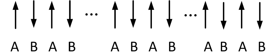
Figure 1: Two-sub-lattice model: two sub-lattices labeled A and B interpenetrating each other.

For simplicity we only consider the simplest case with $N_{A}=N_{B}=N$, thus the total system size is $2N$. Then the ground state is reduced to an antiferromagnetic ground state which has zero total spin,

$$\mbox{$|S_{A}S_{B};Sm\rangle$}=\mbox{$|\frac{N}{2}\frac{N}{2};00\rangle$}.$$ (16)

This ground state has perfect Neel order, as manifested by the spin-spin correlation function,

$$\begin{split}&\langle\bm{S}_{i}\cdot\bm{S}_{j}\rangle={1\over 4},\hskip 11.38092pti,j\in A\hskip 5.69046pt{\rm or}\hskip 5.69046pti,j\in B;\\ &\langle\bm{S}_{i}\cdot\bm{S}_{j}\rangle=-{1\over 4}-{1\over 4N}\rightarrow-{1\over 4},\hskip 5.69046pti\in A\hskip 5.69046pt{\rm and}\hskip 5.69046ptj\in B.\end{split}$$ (17)

II.2 Reduced density matrix and Entanglement Entropy

We divide the system spatially into two subsystems which are labeled 1 and 2 respectively and study the ground state entanglement entropy $E$ between these two subsystems.

Following is a brief summary about how to solve for the explicit form of the reduced density matrix.

First, we further decompose the system into four parts, $\bm{S}_{A_{1}},\ \bm{S}_{A_{2}},\ \bm{S}_{B_{1}},\ \bm{S}_{B_{2}}$, with

$$\begin{cases}\bm{S}_{A_{1}}=\sum_{i\in A\wedge i\in 1}\bm{S}_{i},\ \ \bm{S}_{A_{2}}=\sum_{i\in A\wedge i\in 2}\bm{S}_{i};\\ \bm{S}_{B_{1}}=\sum_{i\in B\wedge i\in 1}\bm{S}_{i},\ \ \bm{S}_{B_{2}}=\sum_{i\in B\wedge i\in 2}\bm{S}_{i}.\end{cases}$$ (18)

Therefore, these operators satisfy the following relations,

$$\begin{cases}\bm{S}_{A}=\bm{S}_{A_{1}}+\bm{S}_{A_{2}},\ \ \ \bm{S}_{B}=\bm{S}_{B_{1}}+\bm{S}_{B_{2}};\\ \bm{S}_{1}=\bm{S}_{A_{1}}+\bm{S}_{B_{1}},\ \ \ \bm{S}_{2}=\bm{S}_{A_{2}}+\bm{S}_{B_{2}}.\\ \end{cases}$$ (19)

Here we note that, as discussed in the previous section, the spin state within each sub-lattice is ferromagnetic. This means that not only must the total spin quantum numbers of $\bm{S}_{A}$ and $\bm{S}_{B}$ take their maximum values, but the total spin quantum numbers of $\bm{S}_{A_{1}},\ \bm{S}_{A_{2}},\ \bm{S}_{B_{1}}$ and $\bm{S}_{B_{2}}$ must also take their maximum values. More importantly, these values are thus fixed, which enables us to treat the operators $\bm{S}_{A_{1}},\ \bm{S}_{A_{2}},\ \bm{S}_{B_{1}}$ and $\bm{S}_{B_{2}}$ as four single spins, and in what follows we shall denote these operators by their corresponding spin quantum numbers. The problem is then that we are given a four spin state in which the spins $S_{A_{1}}$ and $S_{A_{2}}$ are combined into a state with total spin $S_{A}$ and the spins $S_{B_{1}}$ and $S_{B_{2}}$ are combined in a state with total spin $S_{B}$, and then these two states are combined into a total singlet (resulting in the ground state of our long-range AFM model), and we must express this state in a basis in which the spins $S_{A_{1}}$ and $S_{A_{2}}$ are combined into a state with total spin $S_{1}$ and $S_{B_{1}}$ and $S_{B_{2}}$ are combined into a state with total spin $S_{2}$. This change of basis involves the familiar LS-jj coupling scheme. At this point, to obtain the reduced density matrix we only have to re-express the density matrix in bases of $\langle S_{1}m_{1}S_{2}m_{2};Sm|$ by means of LSjj coupling, then trace out either $\langle S_{1}m_{1}|$ or $\langle S_{2}m_{2}|$.

After some algebra we arrive at:

$$\rho_{1}=tr_{(2)}(\rho)=\sum_{S_{1}m_{1}}|\lambda_{S_{1}m_{1}}|^{2}\mbox{$|S_{1}m_{1}\rangle$}\mbox{$\langle S_{1}m_{1}|$}.$$ (20)

where $\lambda_{S_{1},m_{1}}$ is given by

$$\begin{split}\lambda_{S_{1},m_{1}}&=\bigg{[}\frac{(N+1)(N-N_{1})!N_{1}!}{(N-N_{1}-S_{1})!(N-N_{1}+S_{1}+1)!}\\ &\times\frac{(N-N_{1})!N_{1}!}{(N_{1}-S_{1})!(N_{1}+S_{1}+1)!}\bigg{]}^{\frac{1}{2}}.\end{split}$$ (21)

The bipartite entanglement entropy between subsystems 1 and 2 is then given by,

$$E=E_{1}=-\sum_{S_{1},m_{1}}\lvert\lambda_{S_{1}m_{1}}\rvert^{2}\ln(\lvert\lambda_{S_{1}m_{1}}\rvert^{2}).$$ (22)

Here we note that, although $\lambda_{S_{1}m_{1}}$ is written with an explicit $m_{1}$ dependence, the actual expression is independent of $m_{1}$. As a result, we can eliminate the summation over $m_{1}$ from (23) by multiplying by a factor of $2S_{1}+1$. The final expression for the entanglement entropy is then,

$$E=E_{1}=-\sum_{S_{1}}(2S_{1}+1)\lvert\lambda_{S_{1}}\rvert^{2}\ln(\lvert\lambda_{S_{1}}\rvert^{2}).$$ (23)

Next we shall present the asymptotic behavior of this bipartite entanglement entropy in two limiting cases:

• $N_{1}=N_{2}=N$, this case gives the saturated entropy at fixed $N$ since intuitively $E$ should increase with the subsystem size.

• $1\ll N_{1}\ll N$, in this limit we are considering system’s entanglement with its (much larger) environment, and generically we should be able to find that the entropy should be independent of the total system size as $N\rightarrow\infty$, which is indeed what we find.

By extracting the asymptotic behavior of the eigenvalues of the reduced density matrix $\lambda_{S_{1}}$, turning the summation into integral and forcing the normalization condition of those eigenvalues, the entanglement entropy can be analytically calculated:

$$\begin{split}E_{1}\simeq&-\int_{0}^{\infty}A(2S_{1}+1)e^{-S^{2}_{1}(\frac{1}{N-N_{1}}+\frac{1}{N_{1}})}\\ &\times\ln\left(Ae^{-S^{2}_{1}(\frac{1}{N-N_{1}}+\frac{1}{N_{1}})}\right)dS_{1}\\ \simeq&\ln\left(N_{1}-\frac{N_{1}^{2}}{N}+\frac{1}{2}\sqrt{\frac{\pi(N-N_{1})N_{1}}{N}}\right).\end{split}$$ (24)

First let us consider the equal partition case, which presumably gives the upper limit of the entanglement entropy for a given total system size. For simplicity we set $N$ to be even (note that the total system size is $2N$), thus $N_{1}=\frac{N}{2}$, and $\frac{1}{A}=\frac{1}{4}(N+\sqrt{N\pi})$. So the entanglement entropy becomes,

$$\begin{split}E&=\ln\left(\frac{N}{4}+\frac{1}{4}\sqrt{\pi N}\right)\\ &\simeq\ln N-\ln 4\simeq\ln N-1.38629.\\ \end{split}$$ (25)

For the unequal partition case, $1\ll N_{1}\ll N$, we can expand the entropy as follows,

$$\begin{split}E&\simeq\ln\left[N_{1}\left(1-\frac{N_{1}}{N}+\frac{1}{2}\sqrt{\frac{\pi(1-\frac{N_{1}}{N})}{N_{1}}}\right)\right]\\ &=\ln N_{1}+\ln\left(1-\frac{N_{1}}{N}+\frac{1}{2}\sqrt{\frac{\pi(1-\frac{N_{1}}{N})}{N_{1}}}\right)\\ &\simeq\ln N_{1}-\frac{N_{1}}{N}+O\left(\left(\frac{N_{1}}{N}\right)^{2}\right).\end{split}$$ (26)

From this expression we see that when the assumed condition is satisfied the entropy indeed depends only on the subsystem size to leading order.

II.3 Ferromagnetic model and its entanglement entropy

In this section we consider a ferromagnetic (FM) spin-1/2 model on an arbitrary lattice with $N$ sites,

$$H=-\sum_{i\neq j}J_{ij}\bm{S}_{i}\cdot\bm{S}_{j},$$ (27)

with $J_{ij}>0$. The ground state is the fully magnetized state $|SM\rangle$ with $S=N/2$ and $M=-S,-S+1,\cdots,S$, and is clearly long-range ordered: $\langle\bm{S}_{i}\cdot\bm{S}_{j}\rangle=1/4$. However there is a crucial difference between the FM ground state and the AFM ground state studied earlier: the FM ground state has a finite degeneracy, and thus the system exhibits a non-zero entropy even at zero temperature, $E_{0}=\log(2S+1)=\log(N+1)$, resulting from the density matrix of the entire system,

$$\rho=\frac{1}{2S+1}\sum_{M=-S}^{S}|SM\rangle\langle SM|=\frac{1}{N+1}\sum_{M=-S}^{S}|SM\rangle\langle SM|$$ (28)

In this case the entanglement entropy between two subsystems (1 and 2) is defined in the following manner. We first obtain reduced density matrices for subsystems 1 and 2 by tracing out degrees of freedom in 2 and 1 from $\rho$:

$$\begin{split}&\rho_{1}=tr_{(2)}\rho=\frac{1}{N+1}\sum_{M=-S}^{S}tr_{(2)}(|SM\rangle\langle SM|)\\ &=\frac{1}{N+1}\sum_{M=-S}^{S}\rho_{1M},\\ &\rho_{2}=tr_{(1)}\rho=\frac{1}{N+1}\sum_{M=-S}^{S}tr_{(1)}(|SM\rangle\langle SM|)\\ &=\frac{1}{N+1}\sum_{M=-S}^{S}\rho_{2M},\end{split}$$ (29)

and calculate from them the entropy of the subsystems, $E_{1}$ and $E_{2}$. The entanglement entropy is defined asCramer et al. (2006)

$$E=(E_{1}+E_{2}-E_{0})/2.$$ (30)

For the present case $E_{1}$ and $E_{2}$ can be easily obtained from the following observations. (i) Because the total spin is fully magnetized, so are those in the subsystems: $S_{1}=N_{1}/2$ and $S_{2}=N_{2}/2$. Thus this is a two-spin entanglement problem. (ii) Because the total density matrix $\rho$ is proportional to the identity matrix in the ground state subspace, it is invariant under an arbitrary rotation in this subspace. (iii) As a result the reduced density matrix $\rho_{1}$ is also invariant under rotation in the subspace of subsystem 1 with $S_{1}=N_{1}/2$, and is proportional to the identity matrix in this subspace. Thus

$$\begin{split}\rho_{1}&=\frac{1}{N_{1}+1}\sum_{M_{1}=-\frac{N_{1}}{2}}^{\frac{N_{1}}{2}}|\frac{N_{1}}{2}M_{1}\rangle\langle\frac{N_{1}}{2}M_{1}|\\ \end{split}$$ (31)

and $E_{1}=\log(N_{1}+1)$ (in agreement with Ref. Popkov and Salerno (2005)). Similarly $E_{2}=\log(N_{2}+1)$. Thus

$$E=[\log(N_{1}+1)+\log(N_{2}+1)-\log(N+1)]/2.$$ (32)

We find in both the equal partition ($N_{1}=N_{2}=N/2$) and unequal partition ($N_{1}\ll N_{2}=N-N_{1}$) limits, the entropy grows logarithmically with subsystem size $N_{1}$,

$$\lim_{N_{1}\rightarrow\infty}E\rightarrow{1\over 2}\log(N_{1}).$$ (33)

III Entanglement Entropy of One Dimensional Spinless Free Fermions

III.1 Fermionic Wave Function Approach

III.1.1 Reduced Density Matrix of Spinless Free Fermion on a 1D Lattice

Now let us consider the application of this general formalism to the case of free fermions on a one dimensional lattice of infinite length. The subsystem is taken to N consecutive lattice sites. The Hamiltonian is simply:

$$\mathcal{H}=-t\sum_{n}(\hat{c}_{n+1}^{\dagger}\hat{c}_{n}+\hat{c}_{n}^{\dagger}\hat{c}_{n+1}).$$ (34)

The Hamiltonian is simply diagonalized by performing Fourier transformation. let

$$\hat{c}_{n} = \frac{1}{\sqrt{2\pi}}\int_{-\pi}^{\pi}dke^{-ikn}\tilde{c}_{k}$$ (35)

$$\tilde{c}_{k} = \frac{1}{\sqrt{2\pi}}\sum_{n=-\infty}^{\infty}e^{ikn}\hat{c}_{n}.$$ (36)

We get:

$$\mathcal{H}=-2t\int_{-\pi}^{\pi}dk\cos k\tilde{c}_{k}^{\dagger}\tilde{c}_{k}.$$ (38)

The ground state we will be interested in is to fill the vacuum state up to the Fermi momentum:

$$\begin{split}\mbox{$|\Psi_{0}\rangle$}&=\prod_{k=-k_{f}}^{k_{f}}\tilde{c}_{k}^{\dagger}\mbox{$|0\rangle$}=\left(\prod_{k}(\frac{1}{\sqrt{2\pi}}\sum_{n}e^{-ikn}\hat{c}_{n}^{\dagger})\right)\mbox{$|0\rangle$}\\ \end{split}$$ (39)

But the mode of interest in our problem is the real space state, and according to our general formalism, we shall try to find out our ’state annihilation operator’. For a finite lattice of length N, any state can be written in such a general form:

$$\mbox{$|\{n_{i}\}\rangle$}=\prod_{i}(\hat{c}^{\dagger}_{i})^{n_{i}}\mbox{$|0\rangle$}=\hat{c}_{\{n_{i}\}}^{\dagger}\mbox{$|0\rangle$},$$ (40)

where $i=1,2,...,N$, $n_{i}=\{0,1\}$, $\{n_{i}\}$ denoting a set of occupation numbers.

However, since the ground state $|\Psi_{0}\rangle$ is not vacuum state for $\hat{c}_{i}$, the ’state annihilation operators’ can be spanned as $\hat{a}_{s}=\prod_{i}\hat{O}_{i}$, with $\hat{O}_{i}\in\{\hat{c}_{i},\hat{c}^{\dagger}_{i}\}$. Noticing that Wick’s theorem is valid in this system, one can verify our assertion at the end of last section, and represent $\rho_{s}$ as

$$\rho_{s}=tr_{e}(\rho_{0})=\sum_{\{\hat{O}_{i}\}}\mbox{$\langle(\prod_{i}\hat{O}_{i})^{\dagger}\rangle$}\prod_{i}\hat{O}_{i},\ \text{with }\hat{O}_{i}\in\{\hat{c}_{i},\hat{c}_{i}^{\dagger},\hat{c}_{i}^{\dagger}\hat{c}_{i},\hat{c}_{i}\hat{c}_{i}^{\dagger}\}$$ (41)

Suppose we can find a unitary transformation: $\hat{d}_{m}=\sum_{n=1}^{L}v_{mn}c_{n}$, so that $\mbox{$\langle\hat{d}_{i}\hat{d}_{j}\rangle$}=0,\ \mbox{$\langle\Psi_{0}|\hat{d}_{i}^{\dagger}\hat{d}_{j}|\Psi_{0}\rangle$}=\delta_{ij}\mbox{$\langle\Psi_{0}|\hat{d}_{i}^{\dagger}\hat{d}_{i}|\Psi_{0}\rangle$}$. We can write $\rho_{0}$ in terms of $\{\hat{d}_{i},\hat{d}_{i}^{\dagger}\}$. Then according to Wick’s theorem, and the fact $\mbox{$\langle\hat{c}_{i}\hat{c}_{j}\rangle$}=\mbox{$\langle\hat{d}_{n}\hat{d}_{m}\rangle$}=0$, only terms of $\hat{O}_{i}\in\{\hat{d}_{n}\hat{d}_{n}^{\dagger},\hat{d}_{n}^{\dagger}\hat{d}_{n}\}$ survive. Then it is not hard to see that $\rho_{s}$ can be represented as a product:

$$\rho_{s}=\prod_{i=1}^{L}\left(\mbox{$\langle\Psi_{0}|\hat{d}_{i}\hat{d}_{i}^{\dagger}|\Psi_{0}\rangle$}\hat{d}_{i}\hat{d}_{i}^{\dagger}+\mbox{$\langle\Psi_{0}|\hat{d}_{i}^{\dagger}\hat{d}_{i}|\Psi_{0}\rangle$}\hat{d}_{i}^{\dagger}\hat{d}_{i}\right)$$ (42)

III.1.2 Closed Form for the Entanglement Entropy

According to equation 42, we see

$$\bm{S}(\rho_{s})=-\sum_{i}\left(\mbox{$\langle\Psi_{0}|\hat{d}_{i}\hat{d}_{i}^{\dagger}|\Psi_{0}\rangle$}\ln(\mbox{$\langle\Psi_{0}|\hat{d}_{i}\hat{d}_{i}^{\dagger}|\Psi_{0}\rangle$})+\mbox{$\langle\Psi_{0}|\hat{d}_{i}^{\dagger}\hat{d}_{i}|\Psi_{0}\rangle$}\ln(\mbox{$\langle\Psi_{0}|\hat{d}_{i}^{\dagger}\hat{d}_{i}|\Psi_{0}\rangle$})\right)$$ (43)

Follow the work of Jin and KorepinJin and Korepin (2004), we introduce Majorana operators of $\hat{c}_{i}$s’ and $\hat{d}_{i}$s’

$$\begin{split}c_{2l-1}&=\hat{c}_{l}+\hat{c}_{l}^{\dagger}=\frac{1}{\sqrt{2\pi}}\int_{-\pi}^{\pi}dke^{-ikl}(\tilde{c}_{k}+\tilde{c}_{k}^{\dagger})\\ c_{2l}&=-i(\hat{c}_{l}-\hat{c}_{l}^{\dagger})=\frac{1}{\sqrt{2\pi}}\int_{-\pi}^{\pi}dke^{-ikn}i(\tilde{c}_{k}^{\dagger}-\tilde{c}_{k})\\ d_{2l-1}&=\hat{d}_{l}+\hat{d}_{l}^{\dagger}\text{ and }d_{2l}=-i(\hat{d}_{l}-\hat{d}_{l}^{\dagger}).\\ \end{split}$$ (44)

They satisfy:

$$c_{l}=c_{l}^{\dagger},\ \{c_{l},c_{m}\}=2\delta_{lm},\ \mbox{$\langle c_{l}\rangle$}=0.$$ (45)

The two-point correlation functions now are:

$$\begin{split}\mbox{$\langle c_{2l-1}c_{2m-1}\rangle$}&=\frac{1}{2\pi}\int_{-\pi}^{\pi}dk_{1}dk_{2}e^{-ik_{1}l+ik_{2}m}\mbox{$\langle(\tilde{c}_{k_{1}}+\tilde{c}_{k_{1}}^{\dagger})(\tilde{c}_{k_{2}}+\tilde{c}_{k_{2}}^{\dagger})\rangle$}\\ &=\frac{1}{2\pi}\int_{-\pi}^{\pi}dke^{-i(l-m)k}=\delta_{lm}=\mbox{$\langle c_{2l}c_{2m}\rangle$}\\ \mbox{$\langle c_{2l-1}c_{2m}\rangle$}&=\frac{1}{2\pi}\int_{-\pi}^{\pi}dk_{1}dk_{2}e^{-ik_{1}l+ik_{2}m}\mbox{$\langle(\tilde{c}_{k_{1}}+\tilde{c}_{k_{1}}^{\dagger})(-i)(\tilde{c}_{k_{2}}-\tilde{c}_{k_{2}}^{\dagger})\rangle$}\\ &=\frac{-i}{2\pi}\int_{\pi}^{\pi}dke^{-ik(l-m)}g(k)=-\mbox{$\langle c_{2l}c_{2m-1}\rangle$}\\ g(k)&=\begin{cases}1&\text{if $k>k_{F}$ or $k<-k_{F}$},\\ -1&\text{if $k_{F}>k>-k_{F}$}\\ \end{cases}.\end{split}$$ (46)

So we have:

$$\mbox{$\langle c_{l}c_{m}\rangle$}=\delta_{lm}+i(\mathbf{B}_{L})_{lm},$$ (47)

here $\mathbf{B}_{L}=\mathbf{G}_{L}\otimes\begin{pmatrix}0&1\\ -1&0\\ \end{pmatrix}$, with $\mathbf{G}_{L}=\begin{pmatrix}g_{0}&g_{-1}&\dots&g_{1-L}\\ g_{1}&g_{0}&\ &\vdots\\ \vdots&\ &\ddots&\vdots\\ g_{L-1}&\dots&\dots&g_{0}\\ \end{pmatrix}$

where $g_{l}$ is defined as:

$$g_{l}=\frac{1}{2\pi}\int_{-\pi}^{\pi}dke^{-ilk}g(k),\ g(k)=\begin{cases}1&\text{if $k>k_{F}$ or $k<-k_{F}$},\\ -1&\text{if $k_{F}>k>-k_{F}$}\\ \end{cases}$$ (48)

As we found, once we diagonalize the correlation-function matrix, the entanglement entropy is then given by $-\sum_{i}v_{i}\ln v_{i}$, where $v_{i}$ is the ith eigenvalue of the matrix. However, due to the convention we adopted for the Majorana operators, the transformation is not unitary, but with an extra factor of 2. Thus, in order to ensure the normalization condition of the density matrix, we must divide this factor of 2. Then the closed form for the entanglement entropy is readily given as:

$$S(\rho_{s})=\sum_{i=1}^{L}e(1,\nu_{i})$$ (49)

with

$$e(x,\nu)=-\frac{x+\nu}{2}\ln(\frac{x+\nu}{2})-\frac{x-\nu}{2}\ln(\frac{x-\nu}{2}),\text{ $\nu$' s are eigenvalues of $\mathbf{G}_{L}$}.$$ (50)

However, to obtain all eigenvalues of $\nu_{m}$ directly from the matrix $\mathbf{G}_{L}$ is nontrivial task. Let us introduce

$$D_{L}(\lambda)=\det(\tilde{\mathbf{G}}_{L}(\lambda))\equiv\det(\lambda I_{L}-\mathbf{G}_{L})$$ (51)

$I_{L}$ is a identity matrix of dimension L. It is known that $\mathbf{G}_{L}$ is a Toeplitz matrix (see Böttcher and Silbermann (1990)), i.e. its matrix elements depend solely on the difference between the two indices. Obviously we also have

$$D_{L}(\lambda)=\prod_{m=1}^{L}(\lambda-\nu_{m}).$$ (52)

From the Cauchy residue theorem and the analytical property of $e(x,\nu)$, $S(\rho_{s})$ can be rewritten as

$$S(\rho_{s})=\lim_{\epsilon\rightarrow 0^{+}}\lim_{\delta\rightarrow 0^{+}}\frac{1}{2\pi i}\oint_{c(\epsilon,\delta)}e(1+\epsilon)d\ln D_{L}(\lambda).$$ (53)

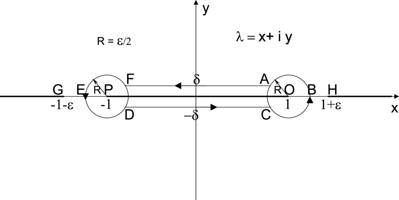
Figure 2: The contour $c(\epsilon,\delta)$. Bold lines ($-\infty,-1-\epsilon$) and ($1+\epsilon,\infty$) are the cuts of integrand $e(1+\epsilon,\lambda)$. Zeros of $D_{L}(\lambda)$ [51] are located on bold line (-1,1) and this line becomes the cut of $\text{d}\log D_{L}(\lambda)$ for $L\rightarrow\infty$. The arrow is the direction of the route of the integral we take and R is the radius of the circle.

Here the contour $c(\epsilon,\delta)$ in Fig.1 encircles all zeros of $D_{L}(\lambda)$, but the function $e(1+\epsilon,\lambda)$ is analytic within the contour. The Toeplitz matrix $\tilde{G}_{L}(\lambda)$ is generated by the function $\tilde{g}(k)$ defined by

$$\tilde{g}(k)=\begin{cases}\lambda-1&-k_{F}<k<k_{F}\\ \lambda+1&k_{F}<k<(2\pi-k_{F})\\ \end{cases}$$ (54)

Once the determinant of the Toeplitz matrix $\mathbf{\tilde{G}}_{L}$ is obtained analytically, one will be able to get a closed analytic result for $S(\rho_{s})$.

III.1.3 The Toeplitz Matrix and the Fisher-Hartwig Conjecture

Toeplitz matrix $T_{\mathrm{L}}[\phi]$ is said to be generated by function $\phi(\theta)$ if

$$T_{\mathrm{L}}[\phi]=(\phi_{i-j}),~{}~{}~{}i,j=1,\cdots,\mathrm{L}-1$$ (55)

where

$$\phi_{l}=\frac{1}{2\pi}\int_{0}^{2\pi}\phi(\theta)e^{-\mathrm{i}l\theta}\mathrm{d}\theta$$ (56)

is the $l$-th Fourier coefficient of generating function $\phi(\theta)$. The determinant of $T_{\mathrm{L}}[\phi]$ is denoted by $D_{\mathrm{L}}$.

Fisher-Hartwig Conjecture: Suppose the generating function of Toeplitz matrix $\phi(\theta)$ is singular in the following form

$$\phi(\theta)=\psi(\theta)\prod_{r=1}^{R}t_{\beta_{r},\,\theta_{r}}(\theta)u_{\alpha_{r},\,\theta_{r}}(\theta)$$ (57)

where

$$t_{\beta_{r},\,\theta_{r}}(\theta) = \exp[-i\beta_{r}(\pi-\theta+\theta_{r})],\qquad\theta_{r}<\theta<2\pi+\theta_{r}$$ (58)

$$u_{\alpha_{r},\,\theta_{r}}(\theta) = \Bigl{(}2-2\cos(\theta-\theta_{r})\Bigr{)}^{\alpha_{r}},\quad\quad\Re\alpha_{r}>-\frac{1}{2}$$ (59)

and $\psi$: $\mathbf{T}\to\mathbf{C}$ is a smooth non-vanishing function with zero winding number. Then as $n\to\infty$, the determinant of $T_{\mathrm{L}}[\phi]$

$$D_{\mathrm{L}}=\left({\cal F}[\psi]\right)^{\mathrm{L}}\left(\prod_{i=1}^{R}{\mathrm{L}}^{\alpha_{i}^{2}-\beta_{i}^{2}}\right){\cal E}[\psi,\{\alpha_{i}\},\{\beta_{i}\},\{\theta_{i}\}],~{}~{}\mathrm{L}\to\infty.$$ (60)

Here ${\cal F}[\psi]=\exp\left(\frac{1}{2\pi}\int_{0}^{2\pi}\ln\psi(\theta)\mathrm{d}\theta\right)$. Further assuming that there exists Weiner-Hopf factorization

$$\psi(\theta)={\cal F}[\psi]\,\psi_{+}\Bigl{(}\exp(\mathrm{i}\theta)\Bigr{)}\,\psi_{-}\Bigl{(}\exp(-\mathrm{i}\theta)\Bigr{)},$$ (61)

then constant ${\cal E}[\psi,\{\alpha_{i}\},\{\beta_{i}\},\{\theta_{i}\}]$ in Eq. 60 can be written as

$${\cal E}[\psi,\{\alpha_{i}\},\{\beta_{i}\},\{\theta_{i}\}] = {\cal E}[\psi]\prod_{i=1}^{R}G(1+\alpha_{i}+\beta_{i})G(1+\alpha_{i}-\beta_{i})/G(1+2\alpha_{i})$$ (62)

$$\times \prod_{i=1}^{R}\biggl{(}\psi_{-}\Bigl{(}\exp(\mathrm{i}\theta_{i})\Bigr{)}\biggr{)}^{-\alpha_{i}-\beta_{i}}\biggl{(}\psi_{+}\Bigl{(}\exp(-\mathrm{i}\theta_{i})\Bigr{)}\biggr{)}^{-\alpha_{i}+\beta_{i}}$$

$$\times \prod_{1\leq i\neq j\leq R}\biggl{(}1-\exp\Bigl{(}\mathrm{i}(\theta_{i}-\theta_{j})\Bigr{)}\biggr{)}^{-(\alpha_{i}+\beta_{i})(\alpha_{j}-\beta_{j})},$$

$G$ is the Barnes $G$-function, ${\cal E}[\psi]=\exp(\sum_{k=1}^{\infty}ks_{k}s_{-k})$, and $s_{k}$ is the $k$-th Fourier coefficient of $\ln\psi(\theta)$. The Barnes $G$-function is defined as

$$G(1+z)=(2\pi)^{z/2}e^{-(z+1)z/2-\gamma_{E}z^{2}/2}\prod_{n=1}^{\infty}\{(1+z/n)^{n}e^{-z+z^{2}/(2n)}\},$$ (63)

where $\gamma_{E}$ is Euler constant and its numerical value is $0.5772156649\cdots$. This conjecture has not been proven for general case. However, there are various special cases for which the conjecture was proven.

For our case, the generating function $\tilde{g}(\theta)$ has two jumps at $\theta=\pm k_{F}$ and it has the following canonical factorization

$$\tilde{g}(\theta)=\psi(\theta)t_{\beta_{1}(\lambda),\,k_{F}}(\theta)t_{\beta_{2}(\lambda),\,-k_{F}}(\theta)$$ (64)

with

$$\psi(\theta)=(\lambda+1)\left(\frac{\lambda+1}{\lambda-1}\right)^{-k_{F}/\pi},~{}~{}~{}\beta(\lambda)=-\beta_{1}(\lambda)=\beta_{2}(\lambda)=\frac{1}{2\pi\mathrm{i}}\ln\frac{\lambda+1}{\lambda-1}.$$ (65)

The function $t$ was defined in Eq. 58. We fix the branch of the logarithm in the following way

$$-\pi\leq\arg\left(\frac{\lambda+1}{\lambda-1}\right)<\pi.$$ (66)

Here we verify the the above factorization expression explicitly. We have two jumps at $\theta=\pm k_{F}$. According to Eq.33, we have two t function:

$$\begin{split}t_{\beta_{1},k_{F}}&=\exp[-i\beta_{1}(\pi-\theta+k_{F})],\ k_{F}<\theta<2\pi+k_{F}\\ t_{\beta_{2},-k_{F}}&=\exp[-i\beta_{2}(\pi-\theta-k_{F})],\ -k_{F}<\theta<2\pi-k_{F}\\ \end{split}$$ (67)

Then $\tilde{g}(\theta)$ is given as:

$$\begin{split}\tilde{g}(\theta)&=(\lambda+1)\left(\frac{\lambda+1}{\lambda-1}\right)^{-k_{F}/\pi}\exp[-i(\frac{1}{2\pi i})\ln(\frac{\lambda+1}{\lambda-1})(\pi-\theta-k_{F})]\\ &\times\exp[-i(\frac{-1}{2\pi i})\ln(\frac{\lambda+1}{\lambda-1})(\pi-\theta+k_{F})]\\ &=(\lambda+1)\left(\frac{\lambda+1}{\lambda-1}\right)^{-k_{F}/\pi}\exp[-\frac{\pi-\theta-k_{F}}{2\pi}\ln(\frac{\lambda+1}{\lambda-1})]\exp[\frac{\pi-\theta+k_{F}}{2\pi}\ln(\frac{\lambda+1}{\lambda-1})]\end{split}$$ (68)

When $\theta\in[-k_{F},k_{F}]$,

$$t_{\beta_{2},-k_{F}}=(\frac{\lambda+1}{\lambda-1})^{-\frac{\pi-\theta-k_{F}}{2\pi}}$$

. However, for $t_{\beta_{,}k_{F}}$, $\theta$ is not defined in this region, but considering periodicity, $\theta\in[2\pi-k_{F},2\pi+k_{F}]$, and to move it into the same region as of $t_{\beta_{2},-k_{F}}$, we must write $t_{\beta_{1},k_{F}}$ as

$$t_{\beta_{1},k_{F}}=(\frac{\lambda+1}{\lambda-1})^{\frac{\pi-(\theta+2\pi)+k_{F}}{2\pi}}=(\frac{\lambda+1}{\lambda-1})^{\frac{k_{F}-\theta-\pi}{2\pi}}$$

Then we have

$$\tilde{g}(\theta)=(\lambda+1)(\frac{\lambda+1}{\lambda-1})^{-1}=\lambda-1,\ \text{when $\theta\in[-k_{F},k_{F}]$}$$ (69)

Similar argument also applies to $\theta\in[k_{F},2\pi-k_{F}]$. And we have verified that the factorization works.

For $\lambda\notin[-1,1]$, we know that $|\Re(\beta_{1}(\lambda))|<\frac{1}{2}$ and $|\Re(\beta_{2}(\lambda))|<\frac{1}{2}$ and Fisher-Hartwig conjecture was PROVEN by E.L. Basor for this case Basor (1979). Therefore, we will call it the theorem instead of conjecture for our application. Hence following the theorem in Eq. 60, the determinant $D_{\mathrm{L}}(\lambda)$ of $\lambda I_{\mathrm{L}}-\mathbf{G}_{\mathrm{L}}$ can be asymptotically represented as

$$D_{\mathrm{L}}(\lambda) = \Bigl{(}2-2\cos(2k_{F})\Bigr{)}^{-\beta^{2}(\lambda)}\left\{G\Bigl{(}1+\beta(\lambda)\Bigr{)}G\Bigl{(}1-\beta(\lambda)\Bigr{)}\right\}^{2}$$ (70)

$$\left\{(\lambda+1)\Bigl{(}(\lambda+1)/(\lambda-1)\Bigr{)}^{-k_{F}/\pi}\right\}^{\mathrm{L}}\mathrm{L}^{-2\beta^{2}(\lambda)}.$$

Here $\mathrm{L}$ is the length of sub-system A and $G$ is the Barnes $G$-function and

$$G(1+\beta(\lambda))G(1-\beta(\lambda))=e^{-(1+\gamma_{E})\beta^{2}(\lambda)}\prod_{n=1}^{\infty}\left\{\left(1-\frac{\beta^{2}(\lambda)}{n^{2}}\right)^{n}e^{\beta^{2}(\lambda)/n^{2}}\right\}.$$ (71)

Therefore,

$$\begin{split}\ln D_{L}(\lambda)&=L(\ln(\lambda+1)-\frac{k_{F}}{\pi}\ln(\lambda+1)+\frac{k_{F}}{\pi}\ln(\lambda-1))-2\beta^{2}(\lambda)\ln L\\ &+2(\ln(G(1+\beta))+\ln(G(1-\beta)))-\beta^{2}(\lambda)\ln(2-2\cos 2k_{F})\\ \end{split}$$ (72)

$$\begin{split}\frac{\partial{\ln D_{L}}}{\partial{\lambda}}&=L(\frac{1-k_{F}/\pi}{\lambda+1}+\frac{k_{F}/\pi}{\lambda-1})-\frac{\partial{\beta(\lambda)}}{\partial{\lambda}}(4\beta(\lambda)\ln L\\ &-2(\frac{G^{\prime}(1+\beta)}{G(1+\beta)}+\frac{G^{\prime}(1-\beta)}{G(1-\beta)})+2\beta(\lambda)\ln(2-2\cos k_{F}))\\ \end{split}$$ (73)

Here our only concern is the first term and the second term which diverge linearly or logarithmically as the size the subsystem.

III.1.4 Asymptotic Behavior of the Entanglement Entropy

Now let us proceed to calculate the leading order of the entanglement entropy according our results.

First, we consider the term grows as subsystem size L. It is not difficult to see that the contribution from this term is actually zero, since the only residues arising from poles at $\lambda=\pm 1$ are just zero.

$$\begin{split}S_{1}(\rho_{s})&=\lim_{\epsilon\rightarrow 0^{+}}\lim_{\delta\rightarrow 0^{+}}\frac{1}{2\pi i}\oint_{c}\text{d}\lambda\left(-\frac{1+\epsilon+\lambda}{2}\ln(\frac{1+\epsilon+\lambda}{2})-\frac{1+\epsilon-\lambda}{2}\ln(\frac{1+\epsilon-\lambda}{2})\right)\\ &\times(\frac{1-k_{F}/\pi}{1+\lambda}-\frac{k_{F}/\pi}{1-\lambda})L\\ &=0\\ \end{split}$$ (74)

Now let us turn to the second leading term of order $\ln L$

$$\begin{split}S_{2}&=\frac{2}{\pi^{2}}\oint\text{d}\lambda\frac{e(1+\epsilon,\lambda)\beta(\lambda)}{(1+\lambda)(1-\lambda)}\ln L\\ &=\frac{2}{\pi^{2}}\oint\text{d}\lambda\left(-\frac{1+\epsilon+\lambda}{2}\ln(\frac{1+\epsilon+\lambda}{2})-\frac{1+\epsilon-\lambda}{2}\ln(\frac{1+\epsilon-\lambda}{2})\right)\\ &\times\frac{1}{2\pi i}\ln\left(\frac{\lambda+1}{\lambda-1}\right)\frac{\ln L}{(1+\lambda)(1-\lambda)}\\ \end{split}$$ (75)

This contour integral can be calculated as follows. First, let us look at Fig.1, noting that

$$\oint_{c(\epsilon,\delta)}\text{d}\lambda(\dots)=\left(\int_{\overrightarrow{AF}}+\int_{\overrightarrow{FED}}+\int_{\overrightarrow{DC}}+\int_{\overrightarrow{CBA}}\right)\text{d}\lambda(\dots),$$ (76)

according to contour integral theory, this contour yields the same result as

$$\oint_{c(\epsilon,\delta)}\text{d}\lambda(\dots)=\left((\int_{\overrightarrow{AF}}+\int_{\overrightarrow{FD}}+\int_{\overrightarrow{DC}}+\int_{\overrightarrow{CA}})+(\int_{\overrightarrow{FEDF}}+\int_{\overrightarrow{ACBA}})\right)\text{d}\lambda(\dots).$$ (77)

The contour $\int_{\overrightarrow{FEDF}}$ and $\int_{\overrightarrow{ACBA}}$ are merely closed circles around the points $\pm 1$. As we take the limit $\epsilon\rightarrow 0^{+}$, they shrink and contain only this two points. Using Cauchy’s residue theorem, it is easy to see that the contribution from these two contours is zero.

So the contour integral is simplified to

$$S_{2}=\frac{2}{\pi^{2}}\left(\int_{-1+i0^{+}}^{1+i0^{+}}-\int_{-1+i0^{-}}^{1+i0^{-}}\right)\text{d}\lambda\frac{e(1+\epsilon,\lambda)\beta(\lambda)}{(1+\lambda)(1-\lambda)}\ln L.$$ (78)

The rest part of the integral function is analytic within the contour, however, $\beta(\lambda)$ could have jumps in its angular part since we fix the branch by requiring $-\pi\leq arg\left(\ln\frac{\lambda+1}{\lambda-1}\right)$.

$$\begin{split}\beta(x+i0^{\pm})&=\frac{1}{2i\pi}\ln\left(\frac{x+i0^{\pm}+1}{x+i0^{\pm}-1}\right)\\ &=\frac{1}{2i\pi}\left(\ln\frac{1+x}{1-x}+\ln\frac{1+\frac{i0^{\pm}}{1+x}}{-1+\frac{i0^{\pm}}{1-x}}\right)\\ &\simeq\frac{1}{2i\pi}\left(\ln\frac{1+x}{1-x}+\ln(-(1+i0^{\pm}))\right)\\ &\simeq\frac{1}{2i\pi}\left(\ln\frac{1+x}{1-x}+\ln(e^{i(\pi+0^{\pm})})\right).\end{split}$$ (79)

Taking into account the branch-cut condition, one immediately see that

$$\begin{split}&\ln e^{i(\pi+0^{+})}=-i(\pi-0^{+})\\ &\ln e^{i(\pi+0^{-})}=i(\pi-0^{-})\\ \end{split}$$ (80)

Therefore, our contour integral can now be written as

$$S_{2}=\frac{2}{\pi^{2}}\int_{-1}^{1}\text{d}\lambda\frac{e(1,\lambda)}{(1+\lambda)(1-\lambda)}\ln L=\frac{1}{3}\ln L$$ (81)

Thus we have obtained the leading order behavior of the entanglement entropy of a segment of length $L$ embedded in an infinite spin-less free fermion lattice. Here we did not calculate the sub-leading terms, however, when $k_{F}$, the Fermi momentum or filling factor, becomes extremely small or very close to 1, they will become more and more important and eventually kill the entanglement’s logarithm dependence on L. The criterion is given by $\mathcal{L}=2L\sin k_{F}\gg 1$.

III.2 Bosonic Approach

III.2.1 Brief Introduction to Bosonization of 1D Spinless Fermion

In this section, we shall briefly introduce the bosonization of fermionic systems in one dimension. We will generally follow von Delft and Schoeller (1998) which follows Haldane’s constructive approach.

For simplicity we will only consider the bosonization of a theory involving only one species of fermions. And bosonization of a theory is possible whenever the following prerequisites are met:

1. The theory can be formulated in terms of a set of fermion creation and annihilation operators with canonical anti-commutation relations: $\{c_{k},c_{k^{\prime}}^{\dagger}\}=\delta_{kk^{\prime}},\ k\in[-\infty,\infty]$;

2. The label $k$ above is a discrete, unbounded momentum index of the form $k=\frac{2\pi}{L}(n_{k}-\frac{1}{2}\delta_{b})$ with $n_{k}\in\mathbb{Z}$ and $\delta_{b}\in[0,2)$. Here $n_{k}$ are integers, $L$ is the length of the system size, and $\delta_{b}$ is a parameter that will determine the boundary condition for the fermion fields defined below.

Obviously the prerequisites here are not directly satisfied by the lattice free fermion model we considered in previous sections. However, they can be satisfied by doing the following procedures: i)performing a particle-hole transformation $c^{\dagger}_{k}\rightarrow\tilde{c}_{k}$ for $k<-k_{F}$, ii) then shifting the Fermi point to $k_{F}=0$, iii) letting the lattice spacing $a\rightarrow 0$, iv) extending definition of $k$ to $(-\infty,\infty)$.

The fermion fields:

$$\psi(x) \equiv (\frac{2\pi}{L})^{1/2}\sum_{k=-\infty}^{\infty}e^{-ikx}c_{k},$$ (82)

$$\text{with inverse }c_{k} = (2\pi L)^{-1/2}\int_{-L/2}^{L/2}dxe^{ikx}\psi(x).$$ (83)

And given a set of discrete $k$’s of the form above, the fields $\psi(x)$ obey the following periodicity condition:

$$\psi(x+L/2)=e^{i\pi\delta_{b}}\psi(x-L/2).$$ (84)

Using the following identityGel’fand and Shilov (1964)

$$\sum_{n\in\mathbb{Z}}e^{iny}=2\pi\sum_{\bar{n}\in\mathbb{Z}}\delta(y-2\pi\bar{n})$$ (85)

we can immediately get the anti-commutation relations:

$$\{\psi(x),\psi^{\dagger}(x^{\prime})\} = \frac{2\pi}{L}\sum_{n\in\mathbb{Z}}e^{-i(x-x^{\prime})(n-\delta_{b}/2)2\pi/L}=2\pi\sum_{\bar{n}\in\mathbb{Z}}\delta(x-x^{\prime}-\bar{n}L)e^{i\pi\bar{n}\delta_{b}};$$ (86)

$$\{\psi(x),\psi(x^{\prime})\} = 0.$$ (87)

Vacuum State $\mbox{$|0\rangle$}_{0}$:

Let $\mbox{$|0\rangle$}_{0}$ be the state defined by the properties

$$c_{k}\mbox{$|0\rangle$}_{0}\equiv 0 k>0,$$ for (88)

$$c^{\dagger}_{k}\mbox{$|0\rangle$}_{0}\equiv 0 k\leq 0.$$ for (89)

We shall call $\mbox{$|0\rangle$}_{0}$ the vacuum state and use it as reference state relative to which the occupations of all other states in Fock space are specified. With this definition we can define the operation of fermion-normal-ordering, to be denoted by ${{}^{*}_{*}}\ {{}^{*}_{*}}$, with respect to this vacuum state: to fermion-normal-order a function of $c$ and $c^{\dagger}$’s, all $c_{k}$ with $k>0$ and all $c_{k}^{\dagger}$ with $k\leq 0$ are to be moved to the right of all other operators(i.e. all all $c_{k}^{\dagger}$ with $k>0$ and all $c_{k}$ with $k\leq 0$), so that:

$$\mbox{${{}^{*}_{*}}ABC\dots{}^{*}_{*}$}=ABC\dots-_{0}\mbox{$\langle 0|ABC\dots|0\rangle$}_{0}\quad\text{for }A,B,C,\dots\in\{c_{k};c_{k}^{\dagger}\}$$ (90)

$\vec{N}$-particle ground state $\mbox{$|\vec{N}\rangle$}_{0}$: Let $\hat{N}$ be the operator that counts the number of electrons relative to $\mbox{$|0\rangle$}_{0}$:

$$\hat{N}\equiv\sum_{k=-\infty}^{\infty}\mbox{${{}^{*}_{*}}c^{\dagger}_{k}c_{k}{{}^{*}_{*}}$}=\sum_{k=-\infty}^{\infty}[c^{\dagger}_{k}c_{k}-{{}_{0}}\mbox{$\langle 0|c^{\dagger}_{k}c_{k}|0\rangle$}_{0}]$$ (91)

The set of all states with the same $\hat{N}$-eigenvalues $N$ will be called the $N$-particle Hilbert space $H_{N}$. It contains infinite number of states, corresponding to different particle-hole excitations. Let us denote all of them by $|N\rangle$. For a given $N$, there is a state which contains no particle-hole excitations. We will denote it as $\mbox{$|N\rangle$}_{0}$. To prevent possible ambiguities in its phase, we define it by the following order:

$$\mbox{$|N\rangle$}_{0}\equiv\begin{cases}c^{\dagger}_{N}c^{\dagger}_{(N-1)}\dots c^{\dagger}_{1}\mbox{$|0\rangle$}_{0}&\text{for }N>0,\\ \mbox{$|0\rangle$}_{0}&\text{for }N=0\\ c_{N+1}c_{(N+2)}\dots c_{0}\mbox{$|0\rangle$}_{0}&\text{for }N<0.\\ \end{cases}$$ (92)

Bosonic operators $b^{\dagger}_{q}$ and $b_{q}$:

$$b^{\dagger}_{q}\equiv\frac{i}{\sqrt{n_{q}}}\sum_{k=-\infty}^{\infty}c^{\dagger}_{k+q}c_{k},\quad b_{q}\equiv\frac{-i}{\sqrt{n_{q}}}\sum_{k=-\infty}^{\infty}c^{\dagger}_{k-q}c_{k},$$ (93)

with $q\equiv\frac{2\pi}{L}n_{q}>0$ where $n_{q}\in\mathbb{Z}^{+}$ is a positive integer. Thus the bosonic creation and annihilation operators are defined for $q>0$ only.

And it is not hard to prove the following bosonic commutation relations:

$$[b_{q},b_{q^{\prime}}] = [b^{\dagger}_{q},b^{\dagger}_{q^{\prime}}]=0,[N_{q},b_{q^{\prime}}]=[N_{q},b^{\dagger}_{k^{\prime}}=0],\quad\text{for all }q,\ q^{\prime};$$ (94)

$$\ [b_{q},b_{q^{\prime}}^{\dagger}] = \sum_{k=-\infty}^{\infty}\frac{1}{n_{q}}(c^{\dagger}_{k+q-q^{\prime}}c_{k}-c^{\dagger}_{k+q}c_{k+q^{\prime}})=\delta_{qq^{\prime}}.$$ (95)

Making a connection with Eq.(93), we could see that in each $N$-particle Hilbert space $H_{N}$, $\mbox{$|N\rangle$}_{0}$ functions as vacuum state for bosonic operators defined above:

$$b_{q}\mbox{$|N\rangle$}_{0}=0,\quad\text{for all}\quad k.$$ (96)

This is because $\mbox{$|N\rangle$}_{0}$ is the $N$-particle ground state and does not contain any particle-hole excitations(bosonic excitations).

With a proper construction of a set of bosonic operators in $k$ space, the construction of boson fields is just straightforward:

$$\varphi(x)\equiv-\sum_{q>0}\frac{1}{\sqrt{n_{q}}}e^{-iqx}b_{q}e^{-aq/2},\quad\varphi^{\dagger}(x)\equiv-\sum_{q>0}\frac{1}{\sqrt{n_{q}}}e^{iqx}b^{\dagger}_{q}e^{-aq/2}.$$ (97)

Here $a>0$ is an infinitesimal regularization parameter which is used to regularize $q\rightarrow\infty$ divergent momentum sums that arise in certain non-normal-ordered expressions and commutators. The following commutation relations can be verified for the boson fields defined above:

$$[\varphi(x),\varphi(x^{\prime})] = [\varphi^{\dagger}(x),\varphi^{\dagger}(x^{\prime})]=0,$$ (98)

$$\ [\varphi(x),\varphi^{\dagger}(x^{\prime})] = \sum_{q>0}\frac{1}{n_{q}}e^{-q[i(x-x^{\prime})+a]}=-\ln[1-e^{-i\frac{2\pi}{L}(x-x^{\prime}-ia)}]$$ (99)

Then consider their Hermitian combination:

$$\phi(x)\equiv\varphi(x)+\varphi^{\dagger}(x).$$ (100)

Check the canonical commutation relation:

$$\begin{split}&[\phi(x),\partial_{x^{\prime}}\phi(x^{\prime})]=i\frac{2\pi}{L}\left(\frac{1}{e^{i\frac{2\pi}{L}(x-x^{\prime}-ia)}-1}+\frac{1}{e^{-i\frac{2\pi}{L}(x-x^{\prime}+ia)}-1}\right)\\ &\xrightarrow{L\rightarrow\infty}2\pi i[\frac{a/\pi}{(x-x^{\prime})^{2}+a^{2}}-\frac{1}{L}]\xrightarrow{a\rightarrow 0}2\pi i[\delta(x-x^{\prime})-\frac{1}{L}],\\ \end{split}$$ (101)

which is exactly the canonical commutation relation for boson fields when $L\rightarrow\infty$.

Bosonization and entanglement entropy

Let us look at the corresponding mapping in real space since the partition of the system is usually carried out in real space. Therefore, to legitimate our use of bosonization to study entanglement entropy, we have to establish the relation between the fermion fields and the boson fields in real space and show that the mapping, at least approximately, preserve the partition of the system.

First, let us look at the fields:

$$\begin{split}\varphi(x)&=\sum_{q>0}\frac{1}{\sqrt{n_{q}}}e^{-iqx}e^{-aq/2}\frac{-i}{\sqrt{n_{q}}}\sum_{k=-\infty}^{\infty}c^{\dagger}_{k-q}c_{k}\\ &=\sum_{q>0}\frac{-i}{n_{q}}e^{-aq/2}e^{-iqx}\sum_{k}\frac{1}{2\pi L}\int^{L/2}_{-L/2}dx_{1}e^{-i(k-q)x_{1}}\psi^{\dagger}(x)\int^{L/2}_{-L/2}e^{ikx_{2}}\psi(x_{2})\\ &=\int dx_{1}dx_{2}\sum_{q>0}\frac{-i}{2\pi Ln_{q}}\psi^{\dagger}(x_{1})\psi(x_{2})\sum_{k}e^{i(-aq/2-qx+qx_{1}-kx_{1}+kx_{2})}\\ &=\int dx_{1}\sum_{n_{q}>0}\frac{-i}{Ln_{q}}\psi^{\dagger}(x_{1})\psi(x_{1})e^{i\frac{2\pi n_{q}}{L}(x_{1}-x-a/2)}\\ &=\int dx_{1}\frac{i}{L}\psi^{\dagger}(x_{1})\psi(x_{1})\ln(1-e^{i\frac{2\pi}{L}(x_{1}-x-a/2)}).\end{split}$$ (102)

It seems that the mapping of fields does not fulfill our requirement. However, if we look at the fermion density operator which is the object one will directly work with when calculating entanglement entropy, we shall see that our requirement is indeed satisfied.

$$\begin{split}\rho_{f}(x)&\equiv\mbox{${{}^{*}_{*}}\psi^{\dagger}(x)\psi(x){{}^{*}_{*}}$}=\frac{2\pi}{L}\sum_{q}e^{-iqx}\sum_{x}\mbox{${{}^{*}_{*}}c^{\dagger}_{k-q}c_{k}{{}^{*}_{*}}$}\\ &=\frac{2\pi}{L}\sum_{q>0}i\sqrt{n_{q}}(e^{-iqx}b_{q}-e^{iqx}b_{q})+\frac{2\pi}{L}\sum_{k}\mbox{${{}^{*}_{*}}c_{k}^{\dagger}c_{k}{{}^{*}_{*}}$}\\ &=\partial_{x}\phi(x)+\frac{2\pi}{L}\hat{N},\quad\text{for $a\rightarrow 0$}.\end{split}$$ (103)

For the whole system, the particle number is conserved, so $\hat{N}$ is just a number. Thus we have justified our utilization of bosonization to study the entanglement entropy in many-fermion systems.

However, we still need to find out corresponding bosonic states of the fermionic states we are interested in. At present we are only interested in fermion ground state at zero temperature, i.e. the Fermi sea. It is the $\mbox{$|0\rangle$}_{0}$ we defined in Eq.(88) and (89) which corresponds to the vacuum state $\mbox{$|N=0\rangle$}_{0}$ of the boson modes.

III.2.2 Entanglement Entropy of free Bosons

In this part,we shall first introduce available analytic result in lattice model. However, though this approach can give a nice analytic expression for entanglement entropy, we can not get desired result explicitly due to technique difficulty. Then we will give a short introduction of the field theory approach, following Calabrese and CardyCalabrese and Cardy (2004).

Lattice Model

Let us consider a system of coupled harmonic oscillators in which the Hamiltonian can generally be written in matrix form as:

$$H=\sum_{i,j}[T_{i,j}p_{i}p_{j}+V_{i,j}x_{i}x_{j}],$$ (104)

where the operators $x_{i}$’s and $p_{i}$’s obey the canonical commutation relation: $[x_{i},p_{j}]=i\delta_{ij}$. Consider its correlation functions of positions and momenta

$$\hat{X}_{n,m}=\mbox{$\langle x_{n}x_{m}\rangle$},\ \hat{P}_{n,m}=\mbox{$\langle p_{n}p_{m}\rangle$}.$$ (105)

The ground state is a Gaussian state, and the multi-point correlation functions observe Wick’s theorem:

$$\mbox{$\langle x_{n}x_{m}x_{k}x_{l}\rangle$}=\mbox{$\langle x_{n}x_{m}\rangle$}\mbox{$\langle x_{k}x_{l}\rangle$}+\mbox{$\langle x_{n}x_{k}\rangle$}\mbox{$\langle x_{m}x_{l}\rangle$}+\mbox{$\langle x_{n}x_{l}\rangle$}\mbox{$\langle x_{m}x_{k}\rangle$}.$$ (106)

This also holds inside the subsystem when we do the truncation. According to Wick’s theorem, this indicates the density matrix of the subsystem, i.e. the reduced density matrix is an exponential of momenta and spatial coordinates. Therefore, in principle we should be able to write the reduced density matrix as:

$$\rho_{s}=\mathcal{K}e^{-H^{\prime}}=e^{-\sum_{i,j}[T_{i,j}^{\prime}p_{i}p_{j}+V_{i,j}^{\prime}x_{i}x_{j}]},$$ (107)

here $\mathcal{K}$ is a normalization factor. It is in general not easy to obtain an explicit analytic expression for $T^{\prime}$ and $V^{\prime}$ due to two reasons: first, even in the simplest case of nearest neighbor coupling, terms that do not conserve particle numbers would arise; second, the transformation must be symplectic . However, for such a Hamiltonian, it is always possible to find a symplectic transformation $c_{j}=\frac{1}{\sqrt{2}}(x_{j}+ip_{j}),a_{k}=\sum_{j}(A_{k}(j)c_{j}+B_{k}^{\dagger}(j)c^{\dagger}_{j}$ which can symplecticly diagonalize the Hamiltonian to the following form:

$$H^{\prime}=\sum_{k}\varepsilon(k)a_{k}^{\dagger}a_{k}.$$ (108)

The eigenvalues $\varepsilon(k)$’s follow from the eigenvalues $\nu_{k}^{2}$ of the $X^{\prime}P^{\prime}$ matrix via

$$\text{cth}(\varepsilon(k)/2)=\nu_{k}/2.$$ (109)

And the entanglement entropy is given by

$$S=\sum_{k}((\nu_{k}+1/2)\ln(\nu_{k}+1/2)-(\nu_{k}-1/2)\ln(\nu_{k}-1/2)).$$ (110)

However, to obtain the full spectrum of the matrix $X^{\prime}P^{\prime}$ and calculate the entanglement entropy is highly non-trivial. No pure analytic approach has been developed, but with the help of numerical methods, one still could reproduce desired scaling law of the entanglement entropy. In the strong coupling limit which corresponds to a massless free field, the scaling behavior has been shown indeed to be $\frac{1}{3}\log L$.

Field Theory ApproachCalabrese and Cardy (2004)

Consider a quantum field theory in one dimension space and one time dimension, described by the following action

$$S=\int\frac{1}{2}\left(-(\pi)^{2}+m^{2}\psi^{2}\right)d^{2}\tau=\int\frac{1}{2}\left((\partial_{\mu}\psi)^{2}+m^{2}\psi^{2}\right)d^{2}\tau,$$ (111)

where $\pi(x)=i\partial_{\mu}\psi$ is the canonical momentum, and satisfies the canonical commutation relation $[\psi(x),\pi(x^{\prime})]=i\delta(x-x^{\prime})$. The density matrix $\rho$ in a thermal state at inverse temperature $\beta$ is

$$\rho(\{\phi(x^{\prime\prime})^{\prime\prime}\}|\{\phi(x^{\prime})^{\prime}\})=Z(\beta)^{-1}\mbox{$\langle\{\phi(x^{\prime\prime})^{\prime\prime}\}|e^{-H}|\{\phi(x^{\prime})^{\prime}\}\rangle$},$$ (112)

where $Z(\beta)=\text{tr}e^{-\beta H}$ is the partition function, and $\{\phi(x)\}$ are the corresponding eigenstates of $\psi(x)$: $\psi(x)\mbox{$|\{\phi(x^{\prime})\}\rangle$}=\phi(x^{\prime})\mbox{$|\{\phi(x^{\prime})\}\rangle$}$. This can be expressed as a (Euclidean) path integral:

$$\rho=Z^{-1}\int[d\phi(x,\tau)]\prod_{x}\delta(\phi(x,0)-\phi(x^{\prime})^{\prime})\prod_{x}\delta(\phi(x,\beta)-\phi(x^{\prime\prime})^{\prime\prime})e^{-S_{E}},$$ (113)

where $S_{E}=\int^{\beta}_{0}L_{E}d\tau$, with $L_{E}$ the euclidean Lagrangian. The normalization factor $Z$, i.e. the partition function is found by setting $\{\psi(x)^{\prime\prime}\}=\{\psi(x)^{\prime}\}$ and integrating over these variables. This has the effect of sewing together the edges along $\tau=0$ and $\tau=\beta$ to form a cylinder of circumference $\beta$.

The reduced density matrix of an interval $A=(x_{i},x_{f})$ can be obtained by sewing together only those points which are not in the interval $A$. This has the effect of leaving an open cut along the line $\tau=0$. For the calculation of entanglement entropy, we need to perform a replica trick here. Instead of calculating $\text{tr}\rho_{A}\log\rho_{A}$, we compute $\rho_{A}^{n}$ first, for any positive integer $n$. To do this, we make $n$ copies of above set-up labeled by an integer $k$ with $1\leq k\leq n$, and sew them together cyclically along the open cut so that $\psi(x)^{\prime}_{k}=\psi(x)^{\prime\prime}_{k+1}(\text{and }\psi(x)^{\prime}_{n}=\psi(x)^{\prime\prime}_{1})$ for all $x\in A$. Let us denote the path integral on this $n$-sheeted structure by $Z_{n}(A)$. Then

$$\text{tr}\rho_{A}^{n}=\frac{Z_{n}(A)}{Z^{n}},$$ (114)

and

$$S_{A}=-\lim_{n\rightarrow 1}\frac{\partial}{\partial n}\frac{Z_{n}(A)}{Z^{n}}.$$ (115)

For a free theory on such n-sheeted geometry, it is easier to use the identity:

$$\frac{\partial}{\partial m^{2}}\log Z_{n}=-\frac{1}{2}\int G_{n}(\mathbf{r},\mathbf{r})d^{2}r,$$ (116)

where $G_{n}(\mathbf{r},\mathbf{r^{\prime}})$ is the Green’s function in the n-sheeted geometry. To obtain $\frac{Z_{n}(A)}{Z^{n}}$, we need $G_{n}-nG_{1}$. The Green’s function can be obtained by solving the Helmholtz equation

$$(-\nabla^{2}_{\mathbf{r}}+m^{2})G_{n}(\mathbf{r},\mathbf{r^{\prime}})=\delta^{2}(\mathbf{r-r^{\prime}})$$ (117)

with n-sheeted geometry. In polar coordinates(2D) this simply means extend the domain of $\theta$ to $[0,2\pi n)$. However, an explicit formula is only available for infinite volume, which means we have to extend the subsystem to a semi-infinite one.

After solving for $G_{n}(\mathbf{r},\mathbf{r^{\prime}})$, let $\mathbf{r^{\prime}=r}$ and perform the integral, we have

$$\frac{\partial}{\partial m^{2}}\log(\frac{Z_{n}}{Z^{n}})=-\frac{1}{2}\int(G_{n}(\mathbf{r,r})-nG_{1}(\mathbf{r,r}))=\frac{1}{24m^{2}}(n-\frac{1}{n}).$$ (118)

This will lead us to the final entanglement entropy

$$S=-\text{tr}\rho\log\rho=-\frac{\partial}{\partial n}\text{tr}\rho^{n}|_{n=1}=-\frac{\partial}{\partial n}(m^{2}a^{2})^{\frac{1}{24}(n-1/n)}|_{n=1}=-\frac{1}{12}\log m^{2}a^{2}.$$ (119)

The power of $a$ is inserted to make the result dimensionless, following Cardy’s convention. In the massless limit where $m\rightarrow 0$ which we are more interested in, physically it is natural to replace $m$ with the inverse subsystem size $L^{-1}$ since the coherent length diverges and subsystem size is the only relevant characteristic size in this problem. Also be careful that we actually dealt with a semi-infinite subsystem which has only one boundary of partition in above approach. When we consider a more common subsystem which has two boundaries of partition, we want to double this entanglement entropy as it is a boundary effect. Thus we recover the result $S=\frac{1}{3}\log L$ in agreement with other approaches.

IV Next Step: Generalization to Higher Dimensions

IV.1 Violation of Area Law in Fermionic Systems in Higher Dimensions: Known Results

In Wolf’s workWolf (2006), he considers a general number preserving quadratic Hamiltonian

$$H=\sum_{\alpha,\beta}T_{\alpha,\beta}c^{\dagger}_{\alpha}c_{\beta},T=T^{\dagger},$$ (120)

describing Fermions on a d-dimensional cubic lattice, so that each component of the vector $\alpha$, $\beta$ corresponds to one spatial dimension. Peschel et al.Peschel (2003); Cheong and Henley (2004) obtain a general result on the reduced density matrix of such a Hamiltonian

$$\rho_{s}=\mathcal{K}e^{-H^{\prime}}=\mathcal{K}e^{-\sum_{i,j}H^{\prime}_{i,j}c_{i}^{\dagger}c_{j}},$$ (121)

where $H^{\prime}=\log(1-C)/C$, $C=(c_{i}^{\dagger}c_{j})_{i,j}$. Here all the indices could be vectors when we consider dimension $d>2$. Their argument is quite general and applies to not only arbitrary dimensions but finite temperature as well. And from this $\rho_{s}$ one can easily derive the following expression of entanglement entropy:

$$S = \sum_{j=1}^{L^{d}}h(\lambda_{j}),$$ (122)

$$h(x) = -\frac{1+x}{2}\log\frac{1+x}{2}-\frac{1-x}{2}\log\frac{1-x}{2},$$ (123)

which are general and also hold for systems of higher dimensions. $\lambda_{j}$’s are eigenvalues of the correlation matrix $C$. However, a direct computation of $S$ via the diagonalization of $C$ is highly non-trivial even in the simplest case as we have seen in previous sections. Wolf’s argument is based on the upper bound and lower bound behaviors of the entropy function $h(\lambda)$.

His conclusion is that

$$c_{-}L^{d-1}\log L\leq S\leq c_{+}L^{d-1}(\log L)^{2},$$ (124)

with constants $c_{\pm}$ depending only on the Fermi sea. This result requires that the Fermi surface must be regular enough, i.e. not fractal nor Cantor-like.

Gioev and Klich provide a more specific expression for the scaling behavior of fermion entanglement entropy by making a connection with Widom conjecture

$$S\sim\frac{L^{d-1}\log L}{(2\pi)^{d-1}}\frac{1}{12}\int_{\partial\Omega}\int_{\partial\Gamma}\lvert n_{x}\cdot n_{p}\rvert dS_{x}dS_{p},.$$ (125)

This has been verified numericallyBarthel et al. (2006a); Li et al. (2006).

IV.2 Outlook: Bosonization in Higher Dimensions and Entanglement Entropy

High Dimension Bosonization We have shown basics of one-dimensional bosonization in previous sections. Bosonization in arbitrary dimensions was first formulated by HaldaneHaldane (1994) (for a review see Houghton et al. (2000)). The basic idea of bosonization in $d>1$ dimensions is to divide the Fermi surface into small segments S with height $\lambda$ in the radial direction and area $\Lambda^{d-1}$ along the Fermi surface. These two scale must satisfy the following condition:

$$k_{F}\gg\Lambda\gg\lambda.$$ (126)

Then we focus on the low energy physics relative to Fermi energy. This is done by integrating out the high momentum (energy) degrees of freedom to get the effective Hamiltonian. Working with the effective Hamiltonian within each segment S, we will find ourselves in a situation similar to that near the Fermi points in one-dimensional systems. For small momentum transfer $q\ll\lambda$, it is again possible to pair up the particle-hole excitations in a bosonic way as in one-dimension case within small correction as long as the prerequisites are fulfilled.

Possibility of Entanglement Entropy via Bosonization

The possibility of application of bosonization in higher dimensions arises from several aspects:

1. According to results in one-dimensional system (given by Korepin et al.) where correction with respect to the Fermi energy $\varepsilon_{f}$ is included, we see that the singular behavior, i.e. the $\log L$ scaling, only emerges when $\varepsilon_{f}$ becomes big enough or the Fermi sea becomes deep enough. This is one of the most fundamental requirements for the 1-d bosonization to work properly. In one dimension bosonization becomes exact when we have a infinitely deep Fermi sea;

2. The agreement on the scaling behavior of entanglement entropy in free fermion systems and free boson systems;

3. There has been successful application of bosonization in the calculation of entanglement entropy of two dimensional free Dirac fieldsCasini et al. (2005). Even though in that case the Fermi surface is absent, it is still nonetheless a strong indication that bosonization in higher dimensions could work in the presence of Fermi surface.

The advantage of bosonization approach is that it could take into account the interactions in arbitrary dimensions.

References

- Amico et al. [2008] L. Amico, R. Fazio, A. Osterloh, and V. Vedral. Entanglement in many-body systems. Reviews of Modern Physics, 80(2):517, 2008. doi: 10.1103/RevModPhys.80.517. URL http://link.aps.org/abstract/RMP/v80/p517.
- Barthel et al. [2006a] T. Barthel, M.-C. Chung, and U. Schollwoeck. Entanglement scaling in critical two-dimensional fermionic and bosonic systems. Physical Review A, 74:022329, 2006a. URL doi:10.1103/PhysRevA.74.022329.
- Barthel et al. [2006b] T. Barthel, S. Dusuel, and J. Vidal. Entanglement entropy beyond the free case. Physical Review Letters, 97(22):220402, 2006b. doi: 10.1103/PhysRevLett.97.220402. URL http://link.aps.org/abstract/PRL/v97/e220402.
- Basor [1979] E. L. Basor. A localization theorem for toeplitz determinants. Indiana Univ. Math. J., 28:975, 1979.
- Bell [1987] J. Bell. Speakable and unspeakable in Quantum Mechanics. Cambridge University Press, Cambridge, 1987.
- Bombelli et al. [1986] L. Bombelli, R. K. Koul, J. Lee, and R. D. Sorkin. Quantum source of entropy for black holes. Phys. Rev. D, 34(2):373–383, Jul 1986. doi: 10.1103/PhysRevD.34.373.
- Bonesteel and Yang [2007] N. E. Bonesteel and K. Yang. Infinite-randomness fixed points for chains of non-abelian quasiparticles. Physical Review Letters, 99(14):140405, 2007. doi: 10.1103/PhysRevLett.99.140405. URL http://link.aps.org/abstract/PRL/v99/e140405.
- Böttcher and Silbermann [1990] A. Böttcher and B. Silbermann. Analysis of Toeplitz Operators. Springer-Verlag, 1990.
- Calabrese and Cardy [2004] P. Calabrese and J. Cardy. Entanglement entropy and quantum field theory. Journal of Statistical Mechanics Theory and Experiment, 0406:002, 2004. URL http://www.citebase.org/abstract?id=oai:arXiv.org:hep-th/0405152.
- Casini et al. [2005] H. Casini, C. D. Fosco, and M. Huerta. Entanglement and alpha entropies for a massive dirac field in two dimensions. Journal of Statistical Mechanics Theory and Experiment, 0507:007, 2005. URL http://www.citebase.org/abstract?id=oai:arXiv.org:cond-mat/0505563.
- Cheong and Henley [2004] S.-A. Cheong and C. L. Henley. Many-body density matrices for free fermions. Phys. Rev. B, 69(7):075111, Feb 2004. doi: 10.1103/PhysRevB.69.075111.
- Cramer et al. [2006] M. Cramer, J. Eisert, M. B. Plenio, and J. D. ig. Entanglement-area law for general bosonic harmonic lattice systems. Physical Review A (Atomic, Molecular, and Optical Physics), 73(1):012309, 2006. doi: 10.1103/PhysRevA.73.012309. URL http://link.aps.org/abstract/PRA/v73/e012309.
- Ding et al. [2008] W. Ding, N. E. Bonesteel, and K. Yang. Block entanglement entropy of ground states with long-range magnetic order. Physical Review A (Atomic, Molecular, and Optical Physics), 77(5):052109, 2008. doi: 10.1103/PhysRevA.77.052109. URL http://link.aps.org/abstract/PRA/v77/e052109.
- Einstein et al. [1935] A. Einstein, B. Podolsky, and N. Rosen. Can quantum-mechanical description of physical reality be considered complete? Phys. Rev., 47(10):777–780, May 1935. doi: 10.1103/PhysRev.47.777.
- Feiguin et al. [2007] A. Feiguin, S. Trebst, A. W. W. Ludwig, M. Troyer, A. Kitaev, Z. Wang, and M. H. Freedman. Interacting anyons in topological quantum liquids: The golden chain. Physical Review Letters, 98(16):160409, 2007. doi: 10.1103/PhysRevLett.98.160409. URL http://link.aps.org/abstract/PRL/v98/e160409.
- Fradkin and Moore [2006] E. Fradkin and J. E. Moore. Entanglement entropy of 2d conformal quantum critical points: Hearing the shape of a quantum drum. Physical Review Letters, 97(5):050404, 2006. doi: 10.1103/PhysRevLett.97.050404. URL http://link.aps.org/abstract/PRL/v97/e050404.
- Freedman and Clauser [1972] S. J. Freedman and J. F. Clauser. Experimental test of local hidden-variable theories. Phys. Rev. Lett., 28(14):938–941, Apr 1972. doi: 10.1103/PhysRevLett.28.938.
- Gel’fand and Shilov [1964] I. M. Gel’fand and G. E. Shilov. Generalized Functions, volume 1. Academic Press, New York, 1964.
- Gioev and Klich [2006] D. Gioev and I. Klich. Entanglement entropy of fermions in any dimension and the widom conjecture. Physical Review Letters, 96(10):100503, 2006. doi: 10.1103/PhysRevLett.96.100503. URL http://link.aps.org/abstract/PRL/v96/e100503.
- Haldane [1994] F. D. M. Haldane. Luttinger’s theorem and bosonization of the fermi surface. Proceedings of the International School of Physics ”Enrico Fermi”, Course CXXI ”Perspectives in Many-Particle Physics” eds. R. A. Broglia and J. R. Schrieffer (North-Holland, Amsterdam 1994) pp 5-29, page 17, 1994. URL http://www.citebase.org/abstract?id=oai:arXiv.org:cond-mat/0505529.
- Holzhey et al. [1994] C. Holzhey, F. Larsen, and F. Wilczek. Geometric and renormalized entropy in conformal field theory. Nuclear Physics B, 424:443, 1994. URL http://www.citebase.org/abstract?id=oai:arXiv.org:hep-th/9403108.
- Houghton et al. [2000] A. Houghton, H. J. Kwon, and J. B. Marston. Multidimensional bosonization. Advances in Physics, 49:141, 2000. URL http://www.citebase.org/abstract?id=oai:arXiv.org:cond-mat/9810388.
- Its et al. [2005] A. R. Its, B. Q. Jin, and V. E. Korepin. Entanglement in xy spin chain. MATH.GEN., 38:2975, 2005. URL http://www.citebase.org/abstract?id=oai:arXiv.org:quant-ph/0409027.
- Jin and Korepin [2004] B.-Q. Jin and V. Korepin. Quantum spin chain, toeplitz determinants and the fisher-hartwig conjecture. Journal of Statistical Physics, 116:79, 2004. URL http://arxiv.org/abs/quant-ph/0304108.
- Kitaev and Preskill [2006] A. Kitaev and J. Preskill. Topological entanglement entropy. Physical Review Letters, 96(11):110404, 2006. doi: 10.1103/PhysRevLett.96.110404. URL http://link.aps.org/abstract/PRL/v96/e110404.
- Latorre et al. [2005] J. I. Latorre, R. Orús, E. Rico, and J. Vidal. Entanglement entropy in the lipkin-meshkov-glick model. Physical Review A (Atomic, Molecular, and Optical Physics), 71(6):064101, 2005. doi: 10.1103/PhysRevA.71.064101. URL http://link.aps.org/abstract/PRA/v71/e064101.
- Levin and Wen [2006] M. Levin and X.-G. Wen. Detecting topological order in a ground state wave function. Physical Review Letters, 96(11):110405, 2006. doi: 10.1103/PhysRevLett.96.110405. URL http://link.aps.org/abstract/PRL/v96/e110405.
- Li et al. [2006] W. Li, L. Ding, R. Yu, T. Roscilde, and S. Haas. Scaling behavior of entanglement in two- and three-dimensional free-fermion systems. Physical Review B (Condensed Matter and Materials Physics), 74(7):073103, 2006. doi: 10.1103/PhysRevB.74.073103. URL http://link.aps.org/abstract/PRB/v74/e073103.
- Nielsen and Chuang [2000] M. A. Nielsen and I. Chuang. Quantum Computation and Quantum Information. Cambridge University Press, Cambridge, 2000.
- Peres [1993] A. Peres. Quantum Theory: Concepts and Methods. Kluwer, Dordrecht, 1993.
- Peschel [2003] I. Peschel. Calculation of reduced density matrices from correlation functions. MATH.GEN., 36:L205, 2003. URL http://www.citebase.org/abstract?id=oai:arXiv.org:cond-mat/0212631.
- Popkov and Salerno [2005] V. Popkov and M. Salerno. Logarithmic divergence of the block entanglement entropy for the ferromagnetic heisenberg model. Physical Review A (Atomic, Molecular, and Optical Physics), 71(1):012301, 2005. doi: 10.1103/PhysRevA.71.012301. URL http://link.aps.org/abstract/PRA/v71/e012301.
- Refael and Moore [2004] G. Refael and J. E. Moore. Entanglement entropy of random quantum critical points in one dimension. Phys. Rev. Lett., 93(26):260602, Dec 2004. doi: 10.1103/PhysRevLett.93.260602.
- Santachiara et al. [2006] R. Santachiara, F. Stauffer, and D. Cabra. Entanglement properties and moment distributions of a system of hard-core anyons on a ring. J. Stat. Mech.: Theory Exp., page L06002, 2006. doi: 10.1088/1742-5468/2007/05/L05003. URL http://www.citebase.org/abstract?id=oai:arXiv.org:cond-mat/0610402.
- Srednicki [1993] M. Srednicki. Entropy and area. Phys. Rev. Lett., 71(5):666–669, Aug 1993. doi: 10.1103/PhysRevLett.71.666.
- Vidal et al. [2003] G. Vidal, J. I. Latorre, E. Rico, and A. Kitaev. Entanglement in quantum critical phenomena. Phys. Rev. Lett., 90(22):227902, Jun 2003. doi: 10.1103/PhysRevLett.90.227902.
- Vidal et al. [2007] J. Vidal, S. Dusuel, and T. Barthel. Entanglement entropy in collective models. Journal of Statistical Mechanics: Theory and Experiment, 2007(01):P01015, 2007. URL http://stacks.iop.org/1742-5468/2007/P01015.
- von Delft and Schoeller [1998] J. von Delft and H. Schoeller. Bosonization for beginners — refermionization for experts. Annalen Phys., 7:225–305, 1998.
- Widom [1982] H. Widom. On a class of integral operators with discontinuous symbol. Operator Theory: Adv. Appl., 4:477, 1982.
- Wolf [2006] M. M. Wolf. Violation of the entropic area law for fermions. Physical Review Letters, 96(1):010404, 2006. doi: 10.1103/PhysRevLett.96.010404. URL http://link.aps.org/abstract/PRL/v96/e010404.
- Wolf et al. [2008] M. M. Wolf, F. Verstraete, M. B. Hastings, and J. I. Cirac. Area laws in quantum systems: mutual information and correlations. Phys. Rev. Lett., 100,:070502, 2008.
- Yusuf et al. [2004] E. Yusuf, A. Joshi, and K. Yang. Spin waves in antiferromagnetic spin chains with long-range interactions. Phys. Rev. B, 69(14):144412, Apr 2004. doi: 10.1103/PhysRevB.69.144412.