Stochastic Quantum Molecular Dynamics

Abstract

An approach to correlated dynamics of quantum nuclei and electrons both in dynamical interaction with external environments is presented. This stochastic quantum molecular dynamics rests on a theorem that establishes a one-to-one correspondence between the total ensemble-averaged current density of interacting nuclei and electrons and a given external vector potential. The theory allows for a first-principles description of phenomena previously inaccessible via standard quantum molecular dynamics such as electronic and nuclear relaxation in photochemistry, dissipative correlated electron-ion dynamics in intense laser fields, nuclear dephasing, etc. As a demonstration of the approach, we discuss the rotational relaxation of 4-(N,N-dimethylamino)benzonitrile in a uniform bath in the limit of classical nuclei.

Quantum molecular dynamics (QMD) approaches, as formulated, e.g., in the Born-Oppenheimer, Ehrenfest or Car-Parrinello methods, have proved to be extremely useful tools to study the dynamics of condensed systems MH00 ; DM02 ; MU06 . In these approaches, the time-evolution of the nuclear degrees of freedom is described by classical Newton-type equations, and the forces acting on the nuclei are typically derived from the electronic wave-function at the instantaneous nuclear configuration. By construction, Born-Oppenheimer and Car-Parinello QMD refer to the electronic ground-state energy, whereas Ehrenfest QMD also allows to take excited electronic wave-functions into account.

In these approaches, energy dissipation and thermal coupling to the environment are usually described with additional thermostats coupled directly to the classical nuclear degrees of freedom. Alternatively, Langevin dynamics can be employed for the time-evolution of the classical nuclei FS01 . Other routes that take environment effects into account are provided by the so-called quantum mechanics/molecular mechanics (QM/MM) methods or by implicit solvation or continuum models (see, e.g., ST07 ). Here, the system of interest is treated quantum mechanically (e.g., with one of the above QMD methods) and the environment is treated explicitly within classical molecular mechanics or, implicitly, via an electrostatic continuum model.

However, all of the above approaches share the common feature that the electronic subsystem is treated always as a closed one, namely it cannot exchange energy and momentum with the environment(s). This is a major limitation since in many physical situations, electrons, being lighter particles than nuclei, respond much faster than the latter ones to dynamical changes in their surrounding. This can lead to electronic transitions among excited states (manifested, e.g., in an effective electron temperature rather different than the ionic one Rob2008 ), which in turn may result in different ionic forces compared to the forces obtained from a closed electronic quantum system at (typically) zero temperature. An even more complicated situation may arise (for instance, for light nuclei in intense laser fields) when the quantum nature of nuclei correlates with the electron dynamics, with the external environment(s) mediating transitions between electron-ion correlated states.

In this paper we propose a novel approach that allows to treat both the electronic and (in principle, quantum) nuclear degrees of freedom, open to one or more environments. Our approach, which we term stochastic quantum molecular dynamics (SQMD), is based on a stochastic current density-functional theory for the combined dynamics of quantum electrons and nuclei. The theorem of stochastic time-dependent current-density-functional theory for a single particle species has been proved in Ref. DiVDA07 ; DiVDA08 . Here we extend it to its non-trivial multi-species case. In the limit of classical nuclei, this formulation reduces to a molecular dynamics scheme which couples the nuclear degrees of freedom to an open electronic system that can exchange energy and momentum with the environment.

In the following, we consider a system of ${N_{\rm e}}$ electrons with coordinates $\underline{\bf r}\equiv\{{\bf r}_{j}\}$ and $N_{n}=\sum_{s}N_{s,n}$ nuclei, where each species $s$ comprises $N_{s,n}$ particles with charges $Z_{s,j}$, masses $M_{s,j}$, $j=1\ldots N_{s,n}$, and coordinates $\underline{\bf R}\equiv\{{\bf R}_{s,j}\}$, respectively. To simplify the notation we denote with $\underline{\bf x}\equiv\{\underline{\bf R},\underline{\bf r}\}$ the combined set of electronic and nuclear coordinates and we use the combined index $\alpha=\{s,j\}$ for the nuclear species. Now, suppose that such a system, subject to a classical electromagnetic field, whose vector potential is ${\bf A}(t)$, is described by the many-body Hamiltonian $\hat{H}_{S}(t)$

$$\begin{split}{\hat{H}}_{S}(t)=&{\hat{T}}_{\rm e}({\bf\underline{r}},t)+{\hat{W}}_{\rm ee}({\bf\underline{r}})+{\hat{U}}_{\rm ext,e}({\bf\underline{r}},t)+{\hat{W}}_{\rm en}({\bf\underline{r}},{\bf\underline{R}})\\ &+{\hat{T}}_{\rm n}({\bf\underline{R}},t)+{\hat{W}}_{\rm nn}({\bf\underline{R}})+{\hat{U}}_{\rm ext,n}({\bf\underline{R}},t),\end{split}$$ (1)

where ${\hat{T}}_{\rm e}(t)$ and ${\hat{T}}_{\rm n}(t)$ are the kinetic energies of electrons and ions, with velocities ${\hat{v}}_{k}(t)=[{\hat{p}}_{k}+e{\bf A}({\hat{{\bf r}}}_{k},t)]/m$ and ${\hat{V}}_{\alpha}(t)=[{\hat{P}}_{\alpha}-Z_{\alpha}{\bf A}({\hat{{\bf R}}}_{\alpha},t)]/M_{\alpha}$, respectively. The electron-electron, electron-nuclear and nuclear-nuclear interaction terms take the form

$$\begin{split}{\hat{W}}_{\rm ee}({\bf\underline{r}})&=\frac{1}{4\pi\epsilon_{0}}\sum_{{j<k}}^{N_{\rm e}}\frac{e^{2}}{|{\hat{{\bf r}}}_{j}-{\hat{{\bf r}}}_{k}|}\equiv\sum_{{j<k}}^{N_{\rm e}}w_{\rm ee}({\hat{{\bf r}}}_{j}-{\hat{{\bf r}}}_{k}),\\ {\hat{W}}_{\rm nn}({\bf\underline{R}})&=\frac{1}{4\pi\epsilon_{0}}\sum_{\alpha<\beta}^{N_{\rm n}}\frac{Z_{\alpha}\,Z_{\beta}}{|{\hat{{\bf R}}}_{\alpha}-{\hat{{\bf R}}}_{\beta}|}\equiv\sum_{{\alpha<\beta}}^{N_{\rm n}}w_{\rm nn}({\hat{{\bf R}}}_{\alpha}-{\hat{{\bf R}}}_{\beta}),\\ {\hat{W}}_{\rm en}({\bf\underline{r}},{\bf\underline{R}})&=-\frac{1}{4\pi\epsilon_{0}}\sum_{k=1}^{N_{\rm e}}\sum_{\alpha=1}^{N_{\rm n}}\frac{e\,Z_{\alpha}}{|{\hat{{\bf r}}}_{k}-{\hat{{\bf R}}}_{\alpha}|}\\ &\equiv\sum_{k=1}^{N_{\rm e}}\sum_{\alpha=1}^{N_{\rm n}}w_{\rm en}({\hat{{\bf r}}}_{k}-{\hat{{\bf R}}}_{\alpha}),\end{split}$$ (2)

and we also allow for external time-dependent scalar potentials ${\hat{U}}_{\rm ext,e}({\bf\underline{r}},t)$ and ${\hat{U}}_{\rm ext,n}({\bf\underline{R}},t)$ that act on electronic and nuclear degrees of freedom, respectively. We then let our system interact with one or more environments represented by a dense spectrum of bosonic degrees of freedom, described by the Hamiltonian $\hat{H}_{B}(t)$. The system and the environments are coupled by a bilinear interaction term $\hat{H}_{SB}=\sum_{j}\hat{S}_{j}\hat{B}_{j}$. Here $\hat{S}$, $\hat{B}$, refer to subsystem and bath operators, respectively . The total Hamiltonian $\hat{H}(t)$ of system and environment then takes the form

$$\hat{H}(t)=\hat{H}_{S}(t)+\hat{H}_{B}(t)+\sum_{j}\hat{S}_{j}\hat{B}_{j}.$$ (3)

By projecting out the bath degrees of freedom, one then obtains the reduced dynamics of the system of interest GN99 . While, quite generally, we could work with the resulting non-Markovian dynamics, for the purpose of this paper, we further make a memory-less approximation for the bath. This leads us to consider the following stochastic many-body Schrödinger equation ($\hbar=1$) 

$$i\partial_{t}\Psi(\underline{\bf x},t)={\hat{H}_{S}}(t)\Psi(\underline{\bf x},t)-\frac{1}{2}i{\hat{S}^{\dagger}}{\hat{S}}\Psi(\underline{\bf x},t)+l(t){\hat{S}}\Psi(\underline{\bf x},t),$$ (4)

where, for simplicity, from now on we consider only the coupling $\hat{S}$ to a single bath, which could be position and/or time dependent. The function $l(t)$ describes a stochastic process with zero ensemble average $\overline{l(t)}=0$ and $\delta$-autocorrelation $\overline{l(t)l(t^{\prime})}=\delta(t-t^{\prime})$. Here $\overline{\cdots}$ describes the statistical average over all members of an ensemble of identical systems with a common initial state $\Psi(\underline{\bf x},t=0)$ (which need not be pure) evolving under Eq. (4). Given the set of potentials ${\hat{U}}_{\rm ext}(\underline{\bf x},t)={\hat{U}}_{\rm ext,e}({\bf\underline{r}},t)+{\hat{U}}_{\rm ext,n}({\bf\underline{R}},t)$ and ${\bf A}(t)$ one can always find a gauge transformation $\Lambda(\underline{\bf x},t)$ so that the scalar potentials vanish at all times, and implying that ${\bf A}(t)\equiv{\bf A}(\underline{\bf x},t)$. In the following we assume that such a gauge transformation has been performed.

At this stage we face a large number of choices for the definition of densities for the construction of a density-functional description of this problem. In fact, certain groupings of nuclear particle and current densities might be better suited to specific physical situations. To maintain flexibility we do not specialize at this point and we prove a theorem for the total current density of electrons and nuclei. To that end, we introduce electronic and nuclear current operators in terms of the velocity fields ${\hat{v}}_{k}(t)$ and ${\hat{V}}_{\alpha}(t)$

$${\hat{j}}{({\bf r},t)}=\frac{e}{2m}\sum_{k}\{{\hat{v}}_{k}(t),\delta(\bf{r}-{\hat{\bf r}}_{k})\}$$ (5)

$${\hat{J}}_{\alpha}{({\bf R},t)}=\frac{Z_{\alpha}}{2M_{\alpha}}\sum_{\stackrel{{\scriptstyle\beta}}{{Z_{\alpha}=Z_{\beta},\,M_{\alpha}=M_{\beta}}}}\{{\hat{V}}_{\beta}(t),\delta(\bf{R}-{\hat{\bf R}}_{\beta})\}$$ (6)

where $\{\hat{p},\hat{q}\}=\hat{p}\hat{q}+\hat{q}\hat{p}$ denotes the usual anticommutator. Likewise, the usual charge density operators can be defined as ${\hat{n}}{({\bf r},t)}=\sum_{k}\delta(\bf{r}-{\hat{\bf r}}_{k})$ for the electrons and ${\hat{N}}_{\alpha}{({\bf R},t)}=\sum_{\beta;Z_{\alpha}=Z_{\beta},\,M_{\alpha}=M_{\beta}}\delta(\bf{R}-{\hat{\bf R}}_{\beta})$ for each nuclear species. The total particle and current density operators of the system can then be written as ${\hat{N}}{({\bf x},t)}={\hat{n}}{({\bf r},t)}+\sum_{\alpha}{\hat{N}}_{\alpha}{({\bf R},t)}$ and ${\hat{\bf J}}{({\bf x},t)}={\hat{j}}{({\bf r},t)}+\sum_{\alpha}{\hat{J}}_{\alpha}{({\bf R},t)}$, respectively.

Solutions of the stochastic Schrödinger equation, Eq. (4), leads to an ensemble of stochastic quantum trajectories which have ensemble-averaged total charge $\overline{N(\underline{\bf x},t)}=\overline{{\langle\,}{\hat{N}}(\underline{\bf x},t){\,\rangle}}$ and current densities $\overline{{\bf J}(\underline{\bf x},t)}=\overline{{\langle\,}{\hat{\bf J}}(\underline{\bf x},t){\,\rangle}}$. Here ${\langle\,}\cdots{\,\rangle}$ denotes the quantum mechanical average.

Contrary to the multi-component formulation of Kreibich et al. KG01 ; KLG08 we will not employ a body-fixed frame for the solution of Eq. (4). This is motivated by the fact that for the initial-value problem of Eq. (4) a general initial condition for the state vector and, in addition, a general time- and space-dependent external vector potential ${\bf A}(\underline{\bf x},t)$ would break the translational and rotational invariance of the original operator $\hat{H}_{S}(t)-{\hat{U}}_{\rm ext}(\underline{\bf x},t)$ in Eq. (1). For our purposes it will therefore be sufficient to work in the laboratory frame. We have now collected all ingredients to state the following result.

Theorem.— For a given bath operator $\hat{S}$, many-body initial state $\Psi(\underline{\bf x},t=0)$ and external vector potential ${\bf A}(\underline{\bf x},t)$, the dynamics of the stochastic Schrödinger equation in Eq. (4) generates ensemble-averaged total particle and current densities $\overline{N(\underline{\bf x},t)}$ and $\overline{{\bf J}(\underline{\bf x},t)}$. Under reasonable physical assumptions, any other vector potential ${\bf A}^{\prime}(\underline{\bf x},t)$ (but same initial state and bath operator) that leads to the same ensemble-averaged total particle and current density, has to coincide, up to a gauge transformation, with ${\bf A}(\underline{\bf x},t)$ .

Proof.— The strategy for the proof of this statement follows the technique introduced in Ref. V04 and also employed in Ref. DiVDA07 . It is thus sufficient to provide the relevant equation of motion and summarize the rationale behind the procedure. The relevant equation of motion is the one for the ensemble-averaged current density

$$\begin{split}&m\frac{\partial}{\partial t}\overline{j_{\alpha}{(\underline{{\bf r}},t)}}+\sum_{\alpha}M_{\alpha}\frac{\partial}{\partial t}\overline{J_{\alpha}{(\underline{{\bf R}},t)}}=\overline{N{(\underline{{\bf x}},t)}}\frac{\partial}{\partial t}{\bf A}{(\underline{{\bf x}},t)}\\[-5.69054pt] &-\overline{{\bf J}{(\underline{{\bf x}},t)}}\times(\nabla\times{\bf A}{(\underline{{\bf x}},t)})+\overline{{\langle\,}{\cal{\hat{F}_{\rm ee}}}{(\underline{{\bf x}},t)}{\,\rangle}}+\overline{{\langle\,}{\cal{\hat{F}_{\rm en}}}{(\underline{{\bf x}},t)}{\,\rangle}}\\ &+\overline{{\langle\,}{\cal{\hat{F}_{\rm nn}}}{(\underline{{\bf x}},t)}{\,\rangle}}+m\overline{{\langle\,}{\cal{\hat{G}}}{(\underline{{\bf r}},t)}{\,\rangle}}+\sum_{\alpha}{M_{\alpha}}\overline{{\langle\,}{\cal{\hat{G}_{{\rm n},\alpha}}}{(\underline{{\bf R}},t)}{\,\rangle}}.\end{split}$$ (7)

Here we have introduced the electron-electron, electron-nuclear and nuclear-nuclear interaction densities

$${\cal{\hat{F}_{\rm ee}}}{(\underline{{\bf x}},t)} = -\sum_{i\neq j}\delta({\bf r}-{\bf r}_{j})\nabla_{j}w_{\rm ee}(r_{i}-r_{j})+m\nabla\cdot\hat{\sigma}_{\rm ee}$$

$${\cal{\hat{F}_{\rm en}}}{(\underline{{\bf x}},t)} = -\sum_{i\neq j}\delta({\bf x}-{\bf x}_{j})\nabla_{j}w_{\rm nn}(x_{i}-x_{j})+m\nabla\cdot\hat{\sigma}_{\rm en}$$ (8)

$$+\sum_{\alpha}M_{\alpha}\nabla\cdot\hat{\sigma}_{\rm ne},$$

where ${\cal{\hat{F}_{\rm nn}}}$ can be obtained from ${\cal{\hat{F}_{\rm ee}}}$ with the replacements ${\bf r}\rightarrow{\bf R}$, $w_{\rm ee}\rightarrow w_{\rm nn}$, $m\nabla\cdot\hat{\sigma}_{\rm ee}\rightarrow\sum_{\alpha}M_{\alpha}\nabla_{\alpha}\cdot\hat{\sigma}_{\rm nn}$. The stress tensors are

$$\begin{split}\hat{\sigma}{{}_{\rm ee}}_{\,i,j}=&-\frac{1}{4}\sum_{k}\{v_{i},\{v_{j},\delta({\bf r}-r_{k})\}\}\\ \hat{\sigma}{{}_{\rm en}}_{\,i,j}=&-\frac{1}{4}\sum_{k}\{v_{i},\{V_{j},\delta({\bf R}-R_{k})\}\},\\ \end{split}$$ (9)

with $\hat{\sigma}{{}_{\rm ne}}_{\,i,j}$ and $\hat{\sigma}{{}_{\rm nn}}_{\,i,j}$ obtained by the exchange ${\bf v}\leftrightarrow{\bf V}$. The remaining terms in Eq. (LABEL:eq:elCurrentEOM) describe the electromagnetic contribution (terms containing ${\bf A}$) and the force densities due to the bath

$$\begin{split}{\cal{\hat{G}}}{(\underline{{\bf r}},t)}={\hat{S}}^{\dagger}{\hat{j}}{(\underline{{\bf r}},t)}{\hat{S}}-\frac{1}{2}\{{\hat{S}}^{\dagger}{\hat{S}},{\hat{j}}{(\underline{{\bf r}},t)}\}\\ {\cal{\hat{G}_{\alpha}}}{(\underline{{\bf R}},t)}={\hat{S}}^{\dagger}{\hat{J}}_{\alpha}{(\underline{{\bf R}},t)}{\hat{S}}-\frac{1}{2}\{{\hat{S}}^{\dagger}{\hat{S}},{\hat{J}}{(\underline{{\bf R}},t)}\}.\\ \end{split}$$ (10)

We can now consider another (primed) system with different initial condition, interaction potentials $w^{\prime}_{\rm ee}$, $w^{\prime}_{\rm nn}$, $w^{\prime}_{\rm en}$ and external vector potential $\hat{\bf A}^{\prime}(\underline{\bf x},t)$. By taking the difference of the equations of motion for the total current densities $\overline{{\bf J}(\underline{\bf x},t)}$ and $\overline{{\bf J^{\prime}}(\underline{\bf x},t)}$ in the unprimed and primed system we arrive at an equation of motion for $\Delta{\bf A}(\underline{\bf x},t)={\bf A}(\underline{\bf x},t)-{\bf A}^{\prime}(\underline{\bf x},t)$. The difference of the vector potentials $\Delta{\bf A}(\underline{\bf x},t)$ can then be shown to be completely determined by the initial condition and a series expansion in time about $t=0$. If the two total current densities of the primed and unprimed system coincide then the unique solution - up to a gauge transformation - is given by $\Delta{\bf A}(\underline{\bf x},t)=0$, when the initial conditions and interaction potentials are the same in the two systems, which proves the theorem.

Discussion.— With this theorem we can now set up a Kohn-Sham (KS) scheme of SQMD where an exchange-correlation (xc) vector potential ${\bf A}_{xc}$ (functional of the initial state, bath operator, and ensemble-averaged current density) acting on non-interacting species, allows to reproduce the exact ensemble-averaged density and current densities of the original interacting many-body system. The resulting charge and current densities would thus contain all possible correlations in the system - if we knew the exact functional. As mentioned before, alternative schemes could be constructed (based on corresponding theorems that could be proved as the above one) by defining different densities and current densities (e.g., by lumping all nuclear densities into one quantity KG01 ). While this may seem a drawback, it is in fact an advantage: some of those schemes may be more appropriate for specific physical problems. Irrespective, one would need to construct xc functionals for the chosen scheme. While this program is possible, it is beyond the scope of the present paper. Therefore, as a first practical implementation of the proposed SQMD, we consider the limit of classical nuclei. This is definitely the simplest case, but it is by no means trivial, and by itself already shows the wealth of physical problems one can tackle with SQMD and the physics one can can extract from it.

In the limit of classical nuclei we then solve the stochastic time-dependent KS equations with given KS Hamiltonian $H_{KS}(\underline{\bf x},t)$ for the electronic degrees of freedom, at each instantaneous set of nuclear coordinates. The result provides the KS Slater determinant $\Psi_{KS}(\underline{\bf x},t)$ from which the forces on nuclei are computed as ${\bf F}_{\alpha}=-\langle\Psi_{KS}(\underline{\bf x},t)|\nabla_{\alpha}\hat{H}_{KS}(\underline{\bf x},t)|\Psi_{KS}(\underline{\bf x},t)\rangle$, for each realization of the stochastic process. One then has direct access to both the average dynamics as well as its distribution . As application we consider the rotational relaxation of 4-(N,N-dimethylamino)benzonitrile (DMABN) in a uniform bath. The relaxation rate that enters the definition of the operator $\hat{S}$ can be derived in principle from the system-bath interaction term $\hat{H}_{SB}$ in Eq. (3) GN99 . In the case of DMABN, relaxation rates are available from experiment DE06 , so that we choose $\tau=100$ fs for our simulation which is within the experimentally observed magnitude. We choose as initial state for the SQMD simulation a rotated dimethyl side-group ($\delta=15^{\circ}$) of DMABN. In Fig. 1 we show the average angle and the binned angle distribution of the dihedral angle $\delta$ for 50 stochastic realizations for bath temperatures of 0K and 300K as a function of time and compare with the closed system solution. The angle distributions in the lower panel of Fig. 1 clearly show the temperature-dependent relaxation of the rotational motion in the open system case. Most importantly, from the transient dynamics of the angle distributions, it is also apparent that the system is not relaxing uniformly to the equilibrium configuration $\delta=0$. Rather, it approaches equilibrium via a series of quasi-bimodal distributions, with the higher temperature “smoothing” these distributions. We also emphasize that the damping of the nuclear motion originates in our simulation exclusively from the forces that are calculated from the electronic open quantum system wave-functions. No additional friction term has been added to the nuclear equation of motion. It would be thus interesting to verify such a prediction with available experimental capabilities.

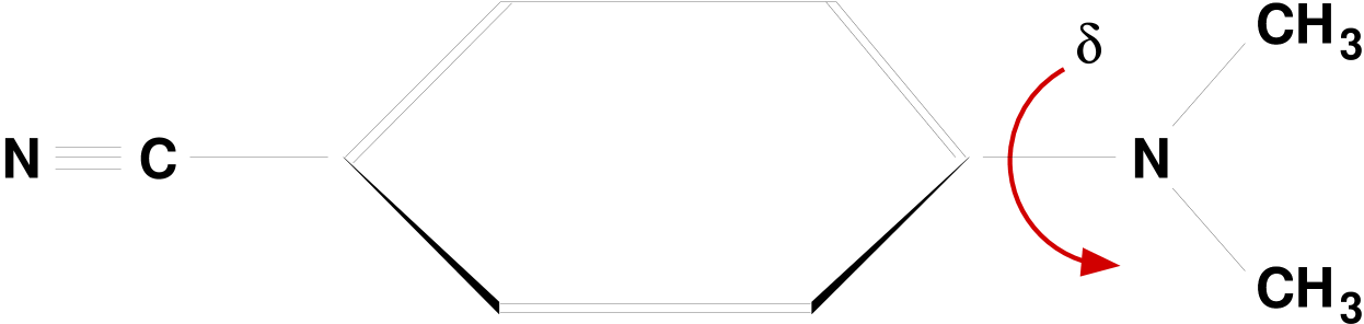
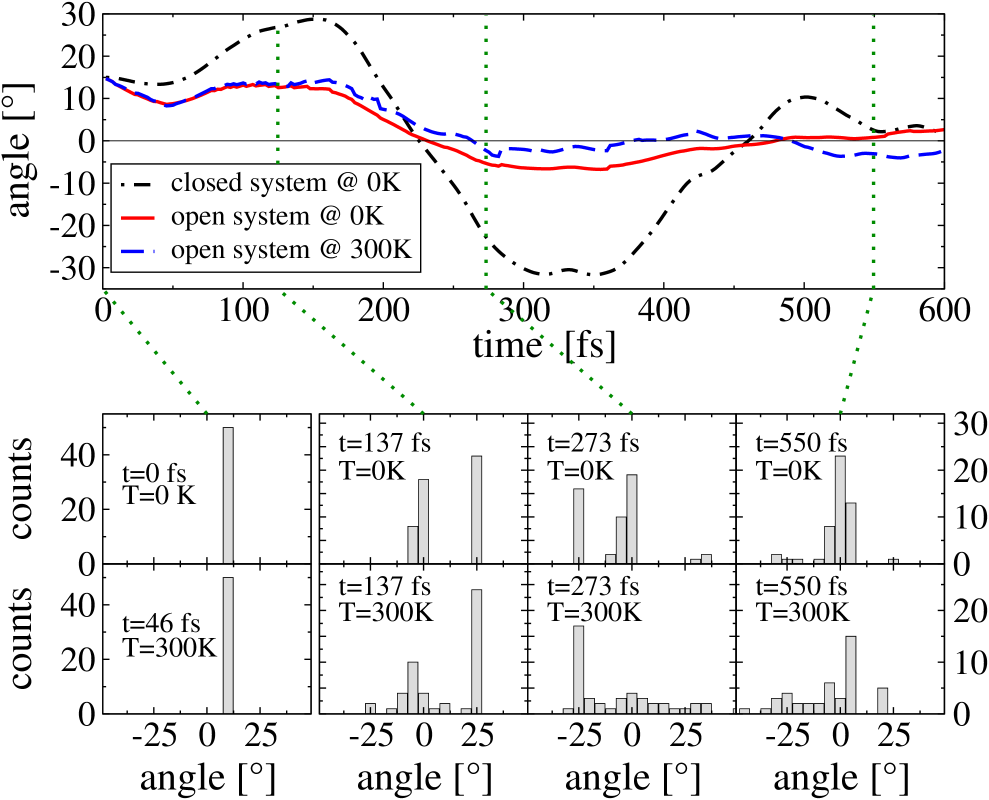
Figure 1: (Color online) Upper panel: schematic illustration of 4-(N,N-dimethylamino)benzonitrile and the dihedral angle $\delta$. Center panel: comparison between the dihedral angle $\delta$ as a function of time for a closed quantum system (dashed line) at 0 K and an open quantum system (solid line) at 300 K. Lower panel: Distributions of the dihedral angle $\delta$ for 50 members of the stochastic ensemble for bath temperatures of 0 K and 300 K at different times (as indicated by the dotted connection lines between the center and the lower panel).

In summary, we have presented a novel quantum molecular dynamics approach which we term stochastic quantum molecular dynamics (SQMD), based on a multi-species theorem of DFT for open quantum systems. SQMD allows to treat both the electronic and nuclear degrees of freedom open to environments, and, in principle, it provides all possible dynamical correlations in the system. In particular, SQMD takes into account energy relaxation and dephasing of the electronic subsystem, a feature lacking in any “standard” MD approach. This opens up the possibility to study a wealth of new phenomena such as local ionic and electronic heating in laser fields, relaxation processes in photochemistry, etc.

We would like to thank Y. Dubi, R. Hatcher and M. Krems for useful discussions. Financial support by Lockheed Martin is gratefully acknowledged.

References

- (1) Dominik Marx and Jürg Hutter (2000) J. Grotendorst (Ed.), John von Neumann Institute for Computing, Jülich, NIC Series, Vol. 1, ISBN 3-00-005618-1, p. 301.
- (2) N. L. Doltsinis, D. Marx, J. of Theo. and Comp. Chem. 1, 319 (2002).
- (3) M. A. L. Marques et. al. (Ed.), Time-Dependent Density Functional Theory (Lecture Notes in Physics) (Springer, 2006), 1st ed.
- (4) B. Smit and D. Frenkel, Understanding Molecular Simulation (Academic Press, London, 2001), 2nd ed.
- (5) H.M. Senn, Thiel W, QM/MM methods for biological systems. In Atomistic Approaches in Modern Biology. (Topics in Current Chemistry, Vol 268). Edited by Reiher M. Berlin: Springer; 2007, p. 173.
- (6) See, e.g., R. D’Agosta and M. Di Ventra, J. Phys. Cond. Matt. 20, 374102 (2008).
- (7) M. Di Ventra and R. D’Agosta, Phys. Rev. Lett 98, 226403 (2007).
- (8) R. D’Agosta and M. Di Ventra, Phys. Rev. B 78, 165105 (2008).
- (9) P. Gaspard, N. Nagaoka, J. Chem. Phys. 111, 5676 (1999).
- (10) T. Kreibich and E.K.U. Gross, Phys. Rev. Lett. 86, 2984 (2001).
- (11) T. Kreibich, R. van Leeuwen and E. K. U. Gross, Phys. Rev. A 78, 022501 (2008).
- (12) G. Vignale, Phys. Rev. B 70, 201102 (2004).
- (13) H.-P. Breuer and F. Petruccione, Theory of open quantum systems (Oxford Univ. Press, 2002), 1st ed.
- (14) A. Castro, et. al. Physica Status Solidi (b), 243, 2465 (2006).
- (15) Yu. V. Pershin, Y. Dubi, and M. Di Ventra, Phys. Rev. B 78, 054302 (2008).
- (16) Sergey I. Druzhinin, et. al., J. Phys. Chem. A 110, 2955 (2006).