Role of emission angular directionality in spin determination of accreting black holes with a broad iron line

Abstract

Aims. The spin of an accreting black hole can be determined by spectroscopy of the emission and absorption features produced in the inner regions of an accretion disc. In this work, we discuss the method employing the relativistic line profiles of iron in the X-ray domain, where the emergent spectrum is blurred by general relativistic effects.

Methods. Precision of the spectra fitting procedure could be compromised by inappropriate accounting for the angular distribution of the disc emission. Often a unique profile is assumed, invariable over the entire range of radii in the disc and energy in the spectral band. An isotropic distribution or a particular limb-darkening law have been frequently set, although some radiation transfer computations exhibit an emission excess towards the grazing angles (i.e., the limb brightening). By assuming a rotating black hole in the centre of an accretion disc, we perform radiation transfer computations of an X-ray irradiated disc atmosphere (NOAR code) to determine the directionality of outgoing X-rays in the $2$–$10$ keV energy band. Based on these computations, we produce a new extension to the ky software package for X-ray spectra fitting of relativistic accretion discs.

Results. We study how sensitive the spin determination is to the assumptions about the intrinsic angular distribution of the emitted photons. The uncertainty of the directional emission distribution translates to $\simeq 20$% uncertainty in the determination of the marginally stable orbit. We implemented the simulation results as a new extension to the ky software package for X-ray spectra fitting of relativistic accretion disc models. Although the parameter space is rather complex, leading to a rich variety of possible outcomes, we find that on average the isotropic directionality reproduces our model data to the best precision. Our results also suggest that an improper use of limb darkening can partly mimic a steeper profile of radial emissivity. We demonstrate these results in the case of XMM-Newton observation of the Seyfert galaxy MCG–6-30-15, for which we construct confidence levels of $\chi^{2}$ statistics, and on the simulated data for the future X-ray IXO mission. Our simulations, with the tentative IXO response, show a significant improvement that can qualitatively enhance the accuracy of spin determination.

1 Introduction

There is now strong evidence suggesting that the radiation of active galactic nuclei as well as some compact binary stars in the Galaxy originates in part from the gas of an accretion disc orbiting around a central black hole (Rees 1998; Kato et al. 1998). A great deal of information about these objects has been obtained via X-rays (Peterson 1997; Krolik 1999). Therefore, reliable models are needed to describe production of high-energy photons emerging from the accretion disc surface and subsequent propagation of these photons towards a distant observer.

Directional distribution of the outgoing radiation is among the important aspects that must be addressed. Limb darkening traditionally refers to the gradual diminution of intensity in the image of the surface of a star as one moves from the centre of the image to the edge. It is a consequence of uneven angular distribution of the radiation flux emerging from the stellar surface (Chandrasekhar 1960; Mihalas 1978). Limb darkening results as a combination of two effects: (i) the density of the surface layers decreases in the outward direction, and (ii) temperature also drops as the distance from the centre of the star increases. The outgoing radiance is therefore distributed in a non-uniform manner. The actual form of the angular distribution depends on the physical mechanism responsible for the emission and the geometrical proportions of the source. The limb darkening law is widely applied also to describe radiation coming from an accretion disc around a black hole. In this case, relativistic effects can significantly enhance the observed anisotropy by bending the light rays and boosting the photon energy in the direction of motion of the emitter. As a result of this interplay between local physics of light emission and the global effects of the gravitational field, different processes contribute to the final (observed) directional anisotropy of the emission.

We consider the angular distribution of the emitted X-rays in the context of accreting black holes. The source is an equatorial accretion disc in which the energy is drawn by conversion of gravitational energy of the orbiting matter gradually sinking into the black hole (Shakura & Syunyaev 1973; Pringle 1981; Frank et al. 2002), and electromagnetic process creating coronal flares and illuminating the underlying accretion disc (Galeev et al. 1979; Nayakshin 2000; Czerny et al. 2004, and further references cited therein). The relevant objects are accreting supermassive black holes in nuclei of galaxies and stellar-mass black holes in compact binary systems (see, e.g., McClintock & Remillard 2006; Miller 2007; Nandra et al. 2007, for broad reviews of the subject). The form of the X-ray spectrum and, in particular, the discrete features at $6$–$7$ keV provide a powerful tool to explore the physical properties of the emitting region, close to the black hole horizon. The line profile often appears to be smeared and asymmetric, with the red wing extending down to $\sim 3$ keV or even less. Spectral modelling can help us to determine the system parameters, namely, the black hole spin (Reynolds et al. 2005; Miller et al. 2009).

It is important to realise that the emission angular directionality probes the physical conditions of the emitting medium. Apart from the above-mentioned temperature stratification, it depends also on the opacity profile. The latter is typically a frequency-dependent quantity, hence the observed radiation also forms at a variable physical depth within the disc. Therefore, the limb darkening/brightening property depends on the wavelength. We take this into account by maintaining the energy resolution in our computations.

The resulting radiation is dominated by X-rays in a few kiloelectronvolt (keV) band, which come from the innermost regions of the accreting system and bear imprints of a strong gravitational field and rapid orbital motion at their origin (Fabian et al. 2000; Fabian 2008). The spectrum is a combination of a multi-colour thermal component from the accreting medium of the disc (Page & Thorne 1974; Li et al. 2005), the power-law component originating from the disc corona (Galeev et al. 1979; Czerny et al. 2004), and the reflection and absorption features arising on the disc surface and in the extended corona along the line of sight (Fabian et al. 1989; Reynolds & Nowak 2003). For active galaxies, the thermal multi-colour black body component dominates in the UV and rarely reaches the sub keV energies. This component, however, occurs at higher energy of the spectrum of black hole binaries.

This paper is organised as follows. Section 2 formulates the model and presents its basic assumptions. Section 3 explores how the constraints on the black hole spin depend on the directionality of the spectrum emerging around the iron line energy. To this end we construct the confidence level diagrams of the $\chi^{2}$ statistics which demonstrate the level of expected sensitivity of the model. First we explore simple analytical approximations of the limb-darkening profile, which do not depend on energy, and then we consider numerical results of our self-consistent radiative transfer computations of both the continuum and the spectral features between $\sim 2$–$10$ keV. We demonstrate the results by “fitting” the artificially simulated data, for which all parameters are perfectly under our control, and by reanalysing the XMM-Newton observation of the Seyfert 1 galaxy MCG–6-30-15. We discuss our results in section 4 and briefly summarise them in section 5.

2 Model assumptions and requisites

2.1 Gravitational field near a rotating black hole

According to general relativity, the gravitational field of a rotating black hole influences the intrinsic spectrum of a nearby source by changing the energy of photons and bending the shape of light rays (Misner et al. 1973). The assumed geometry of the source, i.e. the accretion disc with high orbital velocity near its inner rim, is another factor contributing to significant anisotropy of the emission in the observer’s frame. We remark that geometrical optics provides an appropriate framework describing these effects near astrophysical black holes, where the wavelength of X-rays is much shorter than the typical length-scale of the system represented by the black hole gravitational radius. In the innermost regions of accretion discs, bulk motion of the gas takes place at a significant fraction of the speed of light, indicating that special relativistic aberration and Doppler boosting should be important.

The gravitational field is described by the Kerr metric (Misner et al. 1973, chapt. 33):

$${\rm d}s^{2}=-\frac{\Delta\Sigma}{A}\,{\rm d}t^{2}+\frac{A\,\sin^{2}\theta}{\Sigma}\;\big{(}{\rm d}\phi-\omega\,{\rm d}t\big{)}^{2}+\frac{\Sigma}{\Delta}\,{\rm d}r^{2}+\Sigma\,{\rm d}\theta^{2},$$ (1)

where the Boyer-Lindquist spheroidal coordinates ($t,r,\theta,\phi$) and geometrised units ($c=G=1$) are used. Metric functions are: $\Delta(r)=r^{2}-2r+a^{2}$, $\Sigma(r,\theta)=r^{2}+a^{2}\cos^{2}\theta$, $A(r,\theta)=(r^{2}+a^{2})^{2}-\Delta(r)\,a^{2}\sin^{2}\theta$, and $\omega(r,\theta)=2ar/A(r,\theta)$; $a$ denotes the specific rotational angular momentum (spin) of the central body. These functions are assumed not to be perturbed by gravitational effects of the external matter (accretion disc self-gravity is neglected). Such an assumption is well established if we consider the inner regions of the disc, which within the distance of several gravitational radii contains only very low mass compared to the central black hole mass (Goodman 2003; Karas et al. 2004).

Figure 1: Orbital velocity ${\cal V}(r)$ of co-rotational motion near a rotating black hole, as given by formula (3) for three values of the black-hole dimensionless angular momentum parameter $a$ (spin). The thick part of each curve indicates the range of radii above the marginally stable orbit, $r\geq r_{\rm ms}(a)$, where the circular motion is stable. The thin curve indicates an unstable region at small radii.

Unlike weakly gravitating, non-compact bodies (e.g. main-sequence stars), black holes strongly affect light passing near their horizon. This influence bears not only the signature of black hole mass but it also depends on its rotation via frame-dragging. Although the latter effect is rather weak, it does shape the details of the final spectrum and hence can be employed to measure the black hole angular momentum. The conversion factor from the angular momentum $J_{\rm{}phys}$ (in physical units) to the angular momentum $J$ (in geometrical units) reads: $J=(G/c^{3})J_{\rm{}phys}$. The geometrised dimension of $J$ is the square of the length [cm²].

It is convenient to make all geometrised quantities dimensionless by scaling them with the appropriate power of mass $M$. The dimensionless specific angular momentum, $a\equiv J/M^{2}$, spans the range $-1\leq a\leq 1$, where the positive/negative value refers to the motion co/counter-rotating with respect to the black hole. We will further assume co-rotational motion only ($a\geq 0$). We can scale all lengths by $M$ to reach dimensionless units.

For the Keplerian angular velocity of the orbital motion, we obtain (Bardeen et al. 1972)

$$\Omega_{{}_{\rm{}K}}(r)=\frac{1}{r^{3/2}+a}.$$ (2)

For the linear velocity with respect to a locally non-rotating observer, we have (see Figure 1)

$${\cal V}(r)=\frac{r^{2}-2ar^{1/2}+{a}^{2}}{\Delta^{1/2}\left(r^{3/2}+{a}\right)}.$$ (3)

The velocity at the marginally stable orbit reaches a considerable fraction of the light speed $c$ and has a similar value ${\cal V}(r)\approx 0.5-0.6\,c$ for any value of the angular momentum. For large spin, a small dip develops in the velocity profile near the horizon. Although it is an interesting feature (see Stuchlík et al. 2005), its magnitude is far too small to be recognised in our analysis of the complicated structure of the model $\chi^{2}$ space.

Notice that the above-mentioned interval of $a$-values follows from the assumption, traditionally accepted by astronomers, that we are dealing with a Kerr black hole, for which the outer horizon is located at $r_{+}=1+(1-a^{2})^{1/2}$. Hence, the magnitude of $a$ is thought to be less than unity in order to have a regular horizon and avoid the case of naked singularity, although the latter possibility cannot be straightforwardly rejected just on the basis of spectra fitting.

The standard disc scenario assumes that the accretion disc stops at the innermost stable circular orbit (ISCO, also called the marginally stable orbit), $r_{\rm in}=r_{\rm ms}(a)$, where (Bardeen et al. 1972)

$$r_{\rm ms}=3+Z_{2}-\big{[}\left(3-Z_{1})(3+Z_{1}+2Z_{2}\right)\big{]}^{1\over 2},$$ (4)

$Z_{1}=1+(1-a^{2})^{1\over 3}[(1+a)^{1\over 3}+(1-a)^{1\over 3}]$ and $Z_{2}=(3a^{2}+Z_{1}^{2})^{1\over 2}$. Notice that $r_{\rm ms}(a)$ spans the range of radii from $r_{\rm ms}=1$ for $a=1$ (the case of maximally co-rotating black hole) to $r_{\rm ms}=6$ for $a=0$ (static black hole). As discussed further below, Laor’s (1991) model adopts the standard disc scheme and further assumes that rotation of the black hole is limited by an equilibrium value, $a\dot{=}0.998$, because of capture of photons from the disc (Thorne 1974). This implies $r_{\rm{}ms}\dot{=}1.23$.

2.2 Black-hole signatures in accretion disc radiation

The physical parameters of the black hole – namely, its angular momentum $a$ – are imprinted in the spacetime geometry and they influence the velocity of the orbiting material as well as the radiation propagating through that spacetime. Thus, the observed spectrum is affected – the equivalent width and the centroid energy of spectral lines differ from the value expected on the basis of a purely Newtonian model (e.g. Martocchia et al. 2000; Dabrowski & Lasenby 2001; Miniutti et al. 2003; Vaughan & Fabian 2004, and further references cited therein). In other words, the relativistic effects offer the possibility to reveal the presence of a compact body in the centre of the accretion disc, and to determine its parameters. This assertion is based on an implicit assumption that we can constrain the local physics forming the intrinsic spectrum of the source with sufficient accuracy.

The effects of strong gravity may be concealed from us if the intrinsic spectrum of the accretion disc is not known well enough. This is particularly an issue with respect to the angular momentum determination because the geometrical effect of frame-dragging due to a rotating black hole is a rather subtle one. In order to assess potential inaccuracies, we investigate how sensitive the determination of the $a$ parameter is to the angular distribution of the disc emission, i.e., the limb-darkening (or the limb-brightening) law in the spectral range of $2\lesssim E\lesssim 10$ keV.

Numerical as well as semi-analytical methods were developed and combined to study the spectral features from relativistic accretion discs, especially the profiles of the iron-line complex between $6$–$7$ keV. An important practical attribute from the view point of applicability of any particular method is its implementation within the XSPEC data analysis package (Arnaud 1996). In this context, over almost two decades the most widely used model of the relativistic disc spectral line is the one by Laor (1991), which includes the effects of a rapidly rotating Kerr black hole. The laor model sets the dimensionless angular momentum $a$ to the canonical value of $a=0.998$, so it cannot be the subject of a rigorous data fitting procedure (although see Svoboda et al. 2008).

Although the mathematical properties of the extreme Kerr spacetime ($a^{2}=1$) are significantly different from the sub-extreme case ($a^{2}<1$), the graphs of the redshift factor as well as the emission angle are practically identical. Therefore we do not expect any detectable differences of the observed spectra between these two cases. Secondly, the main effect on the standard accretion disc spectrum and the relativistic broad line formation arises from the assumed link between the inner edge of the disc and the black hole spin parameter (Reynolds & Fabian 2008). Svoboda et al. (2008) have examined the accuracy of the spin fitting using the laor model. They demonstrate that, although such an approach is not self-consistent, the accuracy of the resulting $a$-values is actually quite good.

Dovčiak et al. (2004b) have relaxed the limitation of the laor model regarding the fixed value of the spin. These authors allowed for $a$ to be fitted to the data by $\chi^{2}$ minimisation in a suite of ky models. Furthermore, Beckwith & Done (2004) have developed the kdline, and Brenneman & Reynolds (2006) have developed the kerrdisk models which are endowed with similar functionality. The latter authors performed useful tests demonstrating that ky and kerrdisk give compatible results when they are set to equivalent parameter values. Numerical codes have been developed independently by several other groups (Martocchia et al. 2000; Viergutz 1993; Zakharov & Repin 2004; Fuerst & Wu 2004; Čadež & Calvani 2005) using different techniques. The laor kernel has been recently applied by Miniutti et al. (2007) who reanalysed the prototypical source MCG–6-30-15 using Suzaku observations to determine the relativistic blurring and to measure the black hole parameters. Their results confirm the high value of the spin.

Miller et al. (2009) applied the modelling of relativistic spectral features to estimate the black hole spin from a sample of stellar-mass black holes. They used the joint constraints from both the disc reflection and continuum and found evidence for a broad range of black hole spin parameters.

The angular emissivity law, ${\cal M}(\mu_{\rm e},r_{\rm e},E_{\rm e})$, defines the distribution of the intrinsic intensity outgoing from each radius $r_{\rm e}$ of the disc surface with respect to the perpendicular direction. The emission angle $\theta_{\rm e}=\arccos\mu_{\rm e}$ is measured from the disc normal direction to the equatorial plane, in the disc co-moving frame, i.e. in the local Keplerian frame orbiting with the angular velocity $\Omega_{{}_{\rm{}K}}(r)$. Likewise the intrinsic energy $E_{\rm e}$ is measured with respect to the local frame. The total disc emission can be written in the form of product

$$I(r_{\rm e},\mu_{\rm e},E_{\rm e})\equiv{\cal R}(r_{\rm e})\,\mu_{\rm e}\,{\cal M}(\mu_{\rm e},r_{\rm e},E_{\rm e})\,{\cal E}(E_{\rm e}),$$ (5)

where the radial part is well approximated by a power law,

$${\cal R}(r_{\rm e})=r_{\rm e}^{-q}\qquad(q=\mbox{const}),$$ (6)

and $\mathcal{E}(E_{\rm e})$ is the energy dependence of the locally emitted radiation. When needed we will also use the broken power-law profile which is a combination of two profiles (6) matched at the transition radius, also coded in the ky set of models.

The redshift factor $g$ and the emission angle $\theta_{\rm e}$ are

$$g=\frac{{\cal{C}}}{{\cal{B}}-r^{-3/2}\xi},\quad\theta_{\rm e}=\arccos\frac{g\sqrt{\eta}}{r},$$ (7)

where ${\cal{B}}=1+{a}r^{-3/2}$, ${\cal{C}}=1-3r^{-1}+2{a}r^{-3/2}$; $\xi$ and $\eta$ are constants of motion connected with symmetries of the Kerr spacetime.

The observed radiation flux is then obtained by integrating the intrinsic emission over the entire disc surface, from the inner edge ($r=r_{\rm in}$) to the outer edge ($r=r_{\rm out}$), weighted by the transfer function $T(r_{\rm e},\phi_{\rm e},\theta_{\rm o},a)$ determining the impact of relativistic energy change (Doppler and gravitational) as well as the lensing effect for a distant observer directed along the inclination angle $\theta_{\rm o}$ (see Cunningham 1975; Asaoka 1989; Karas et al. 1992; Karas 2006).

Given the high velocity of the orbital motion and the strong-gravity light bending near the black hole, the effect of directional anisotropy of the local emission is enhanced. For this reason it is important to describe the angular distribution in a correct manner; ad hoc choices of the limb-darkening law may lead to errors in the determination of the model best fit parameters, including the inaccuracy in $a$ parameter which are difficult to control, or they may prevent us from estimating the statistical confidence of the model. In the case of black hole accretion discs, this complication becomes important because the aberration, beaming and light-bending effects grow rapidly towards the inner edge of the disc. Therefore, even a small discrepancy between the assumed and the correct angular emissivity profiles becomes greatly enhanced in the observer frame.

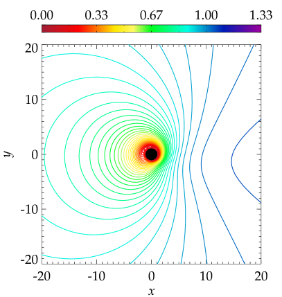
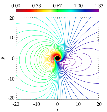
Figure 2: Contours of redshift factor $g(r,\phi)$ near a maximally rotating black hole, $a=1$, depicted in the equatorial plane $(x,y)$. The black hole and the accretion disc rotate counter clock-wise. The inner region is shown up to $r=20$ gravitational radii from the black hole (denoted by dark circle of unit radius around the centre). A distant observer is located towards the top of the figure. Two cases of different observer inclinations are shown. Left: $\theta_{\rm o}=30$ deg. Right: $\theta_{\rm o}=70$ deg. The colour bar encodes the range acquired by $g(r,\phi)$, where $g>1$ corresponds to blueshift (approaching side of the disc), while $g<1$ is for redshift.

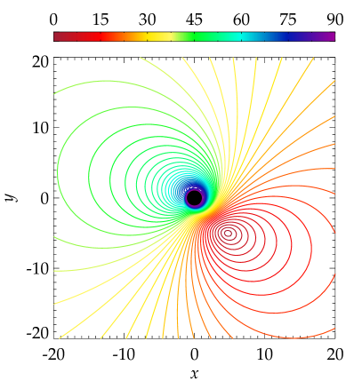
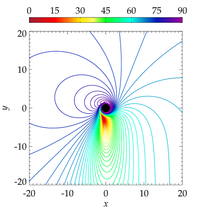
Figure 3: Contours of the local emission angle, $\theta_{\rm e}(r,\phi)$. The same parameters as in the previous figure. The local emission angle spans the entire range, from $0$ to $90$ degrees. This is due to the combined effects of aberration and light bending which grow greatly near the inner rim of the disc. In the inner region the photons are boosted in the direction of rotation and they emerge along grazing angles. Asymptotically, $\theta_{\rm e}(r,\phi)\rightarrow\theta_{\rm o}$ for $r\rightarrow\infty$.

2.3 Effects of the emission angular directionality

In optics, Lambert’s cosine law describes an emitter producing a radiation intensity that is directly proportional to $\mu_{\rm e}$. Lambertian surfaces exhibit the same apparent radiance when viewed from any angle $\theta_{\rm o}$. Likewise, Lambertian scattering refers to the situation when the surface radiates as a result of external irradiation by a primary source and the scattered light is distributed according to the same cosine law. This is, however, a very special circumstance; directionality of the emergent light is sensitive to the details of the radiation mechanism. For example, the classical result of the Eddington approximation for stellar atmospheres states that the effective optical depth of the continuum is $\tau=\frac{2}{3}$, and so the emergent intensity is described by the limb-darkening law, $I(\mu_{\rm e})\propto\mu_{\rm e}+\frac{2}{3}$.

In the case of a fluorescence iron line produced by an illuminated plane-parallel slab, the angular distribution was investigated by various authors (Basko 1978; George & Fabian 1991; Haardt 1993; Ghisellini et al. 1994; Reynolds et al. 2000). In that case a complicated interplay arises among the angular distribution of the primary irradiation, reflection and scattering in the disc atmosphere. Several authors pointed out that it is essential for the reliable determination of the model parameters to determine the angular directionality of the broad line emission correctly. Martocchia et al. (2000) noted, by employing the lamp-post model, that “…the broadening of the observed spectral features is particularly evident when strongly anisotropic emissivity laws, resulting from small $h$ [i.e., the lamp-post elevation above the equatorial plane], are considered.“

The important role of the emission angular directionality was clearly spelled out by Beckwith & Done (2004): “…the angular emissivity law (limb darkening or brightening) can make significant changes to the derived line profiles where light bending is important“ (see their Fig. 9–13). Similarly, Dovčiak et al. (2004a, b) and Beckwith (2005) compared the relativistic broad lines produced under different assumptions about the emission angular directionality. However, to verify the real sensitivity of the models to the mentioned effect of directionality, it is necessary to connect the radiative transfer computations with the spectral fitting procedure, and to carry out a systematic analysis of the resulting spectra, taking into account both the line and the continuum in the full relativistic regime. Here we report on our results from such computations.

Reynolds et al. (2004, sec. 4.3) argue that the combined effect of photoelectric absorption in the disc and Compton scattering in the corona more affect the iron line photons emerging along grazing light rays than continuum photons. They conclude that the line equivalent width should be diminished for observers viewing the accretion disc at high inclination angles. Such a trend can be seen also in the lamp-post model of Matt et al. (1992) and Martocchia et al. (2000, see their Figure 11). However, in the latter work this diminution is less pronounced when we compare it with the case of intrinsically isotropic emissivity.

More recently, Niedźwiecki & Życki (2008) studied the effect of different limb-darkening laws on the iron-line profiles. They point out that the role of emission directionality can be quite significant once the radial emissivity of the line is fixed with sufficient confidence. However, this is a serious assumption. In reality, the radial emissivity is not well constrained by current models.

The angular dependence of the outgoing radiation is determined by the whole interconnection of various effects. We describe them in more detail below (sec. 3.4). Briefly, the conclusion is such that realistic models require numerical computations of the full radiative transfer. We have developed a complete and consistent approach to such radiative transfer computations in the context of the broad iron-line modelling together with the underlying continuum computations. As described in considerable detail below, we performed the extensive computations which are necessary in order to reliably determine the impact of the emission angular anisotropy on spectral fitting results (namely, on the determination of the black hole angular momentum). In particular, we describe detailed results from the investigation of the model goodness (by employing an adequate statistical analysis of the complicated $\chi^{2}$ parameter space). Such the analysis has not been performed so far in previous papers because detailed stepping through the parameter space and proper re-fitting of the model parameters was not possible due to the enormous complexity of the models and extensive computational costs.

Figure 4: Left: directional distribution of the intrinsic emissivity (see sec. 3.1 for details). Right: an example of the directional distribution from the numerical computations, showing results from the reprocessing model with the continuum photon index $\Gamma=1.9$, integrated over $2$–$100$ keV energy range (solid line), and in several different energy sub-ranges (line styles are indicated in the inset). The latter graph demonstrates the presence of limb-brightening effect in comparison with respect to the isotropic emission. This effect is clearly visible as a function of the emission angle $\mu_{\rm e}$, although its magnitude is smaller than the limb-brightening approximation used in the left panel. See sec. 3.4 for details.

In regular stars and their accretion discs, the relativistic effects hardly affect the emerging radiation. The situation is very different in the inner regions of a black hole accretion disc, where the energy shift and gravitational lensing are significant. The observed signal can be boosted or diminished by the Doppler effect combined with gravitational redshift: $I(\mu_{\rm e})/I(\mu_{\rm o})\equiv g^{3}$, where the $g$ values span more than a decade. Figure 2 shows the redshift factor $g$ near the black hole, proving that general relativistic effects indeed change the photon energy significantly.

As mentioned above, many authors have adopted the defining choice (Chandrasekhar 1960; Laor 1991) of the cosine profile for the line angular emissivity: ${\cal M}(\mu_{\rm e},r_{\rm e},E_{\rm e})=1+2.06\,\mu_{\rm e}$. This relation describes the energy-independent limb-darkening type of profile. However, the choice is somewhat arbitrary in the sense that the physical assumptions behind this law are not satisfied at every radius over the entire surface of the accretion disc. It has been argued that the limb-darkening characteristics need to be modified, or even replaced by some kind of limb brightening in the case of X-ray irradiated disc atmospheres with Compton reflection (Haardt 1993; Ghisellini et al. 1994; Życki & Czerny 1994). The latter should include the energy dependence, as the Compton reprocessing of the reflected component plays a significant role. The angle-dependent computations of the Compton reflection demonstrate these effects convincingly (Czerny et al. 2004). Indeed, the same effect is seen also in our computations, as shown in the right panel of Figure 4. The increase of emissivity with the emission angle strongly depends on the ionisation state of the reflecting material, so the actual situation can be quite complex (Goosmann et al. 2007).

A question arises of whether the current determinations of the black hole angular momentum might be affected by the uncertainty in the actual emissivity angular distribution, and to what degree. In fact, this may be of critical concern when future high-resolution data become available from the new generation of detectors. We have therefore carried out a systematic investigation using the ky code to reveal how sensitive the constraints on the dimensionless $a$ parameter are with respect to the possible variations in the angular part ${\cal M}(\mu_{\rm e})$ of the emissivity.

Figure 3 shows the contours of the local emission angle $\theta_{\rm e}$ from the accretion disc, taking into account their distortion by the central black hole and assuming that the emitted photons reach a distant observer at a given view angle $\theta_{\rm o}$. Although the contours are most dramatically distorted near the horizon, where both aberration and light bending effects grow significantly, the emission angle is visibly different from the observer inclination even quite far from the horizon, at a distance of several tens $r_{\rm{}g}$. This is mainly due to special-relativistic aberration which decays slowly with the distance as the disc obeys Keplerian rotation at all radii.

In summary, figures 2–3 demonstrate the main attributes of the photon propagation in black hole spacetime relevant to our problem: the energy shift and the direction of emission depend on the view angle of the observer as well as on the angular momentum of the black hole. Notice that, near the inner rim, the local emission angle is indeed highly inclined towards the equatorial plane where at the same time the outgoing radiation is boosted. These effects are further enhanced by gravitational focusing, which we also take into account in our calculations.

It should be noted that the energy shifts and emission angles near a black hole, such as those shown in Figs. 2–3, have been studied by a number of authors in mutually complementary ways. The figures shown here have been produced by plotting directly the content of FITS format files that are encoded in the corresponding ky XSPEC routines (see Dovčiak (2004), where an atlas of contour plots is presented for different inclinations and spins). Analogous figures were also shown in Beckwith & Done (2004), who depict the dependence of the cosine of the emission angle on the energy shift of the received photon and the emission radius.

The above quoted papers concentrated mainly on the discussion of the energy shifts and the emission directions of the individual photons, or they isolated the role of relativistic effects on the predicted shape of the spectral line profile. They clearly demonstrated that the impact of relativistic effects can be very significant. However, what is still lacking is a more systematic analysis which would reveal how these effects, when integrated over the entire source, influence the results of spectra fitting. To this end one needs to perform an extensive analysis of the model spectra including the continuum component, match the predicted spectra to the data by appropriate spectra fitting procedures, and to investigate the robustness of the fit by varying the model parameters and exploring the confidence contours.

One might anticipate the directional effects of the local emission to be quite unimportant. The argument for such an expectation suggests that the role of directionality should grow with the source inclination, whereas the unobscured Seyfert 1 type AGNs (where the relativistically broadened and skewed iron line is usually expected) are thought to have only small or moderate inclinations. However, this qualitative trend cannot be used to quantitatively constrain the model parameters and perform any kind of precise analysis, needed to determine the black hole spins from current and future high-quality data. Such an analysis has not been performed so far, and we embark on it here for the first time.

3 Iron K$\alpha$ line band examined with different directionalities of the intrinsic emissivity

Figure 5: Left: theoretical profiles of the relativistic line (the kyrline model, without continuum), corresponding to the three cases in the left panel of Fig. 4. The lines are normalised with respect to the height of the blue peak. Model parameters are $a=0.9982$, $q=3$, $r_{\rm in}=r_{\rm ms}(a)=1.23$, $r_{\rm out}=400$, $\theta_{\rm o}=30\deg$, $E_{0}=6.4$ keV. Right: the same as in the left panel, but with the normalisation set in such a way that the radiation flux is identical in all three profiles.

Figure 6: Left: The same as in Fig. 5, but for a narrow ring with $r_{\rm in}\doteq 4.7$, $r_{\rm out}\doteq 4.8$ (other parameters are $a=0.9982$, $q=3$, $\theta_{\rm o}=30\deg$, $E_{0}=6.4$ keV). The lines are normalised with respect to the height of the blue peak. Right: The ratio of the two peak heights for the three cases of the emission angular directionality according to eq. (8) and for the two values of the spin and the inclination angle (crosses and circles are for $\theta_{\rm o}=30\deg$; empty and filled triangles are for $\theta_{\rm o}=60\deg$).

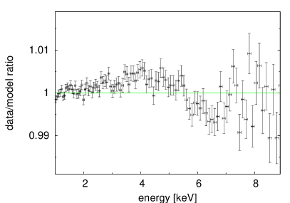
Figure 7: Left: unfolded spectrum generated by the powerlaw + kyrline model with parameters of the line identical as in previous figure. We assumed the limb-brightening profile, i.e. Case 1 of eq. (8). Right: the ratio of the model on the left to the same model with the Case 3 (limb-darkening) profile. The normalisation of the line was allowed to vary during the fit. The $\chi^{2}_{\rm red}$ changed from $1.04$ to $1.30$ between the two cases. The details about the simulation of the data points are the same as described in the section 3.3.

3.1 Approximations to the angular emission profile

We describe the methodology which we adopted in order to explore the effects of the spectral line emission directionality. To this end we first employ simple approximations, neglecting any dependence on the photon energy and the emission radius. We set the line intrinsic emissivity from the planar disc to be described by one of the following angular profiles,

$$\begin{array}[]{l}\mbox{Case 1:}\\ \mbox{Case 2: \rule[-13.00005pt]{0.0pt}{30.00005pt}}\\ \mbox{Case 3:}\end{array}{\cal M}(\mu_{\rm e})=\left\{\begin{array}[]{l}\ln(1+\mu_{\rm e}^{-1})\quad\mbox{\cite[citep]{(\@@bibref{AuthorsPhrase1Year}{1993ApJ...413..680H}{\@@citephrase{ }}{})}}\\ 1\rule[-13.00005pt]{0.0pt}{30.00005pt}\quad\mbox{(locally isotropic emission)}\\ 1+2.06\,\mu_{\rm e}\quad\mbox{\cite[citep]{(\@@bibref{AuthorsPhrase1Year}{1991ApJ...376...90L}{\@@citephrase{ }}{})}}\end{array}\right.$$ (8)

with the radial profiles being a power law ${\cal R}(r_{\rm e})=r_{\rm e}^{-q}$, and ${\cal E}(E_{\rm e})=\delta(E_{\rm e}-E_{0})$. The three cases correspond, respectively, to the limb-brightened, isotropic, and limb-darkened angular profiles of the line emission.

The limb-brightening law by Haardt (1993) describes the angular distribution of a fluorescent iron line emerging from an accretion disc that is irradiated by an extended X-ray source. The relation was obtained from geometrical considerations and agrees well with more detailed Monte-Carlo computations (George & Fabian 1991; Matt et al. 1992). The physical circumstances relevant for the limb-darkening law are different, and we include this case mainly because it is implemented in the laor model and frequently used in the data analysis. The isotropic case, dividing all limb-brightening and limb-darkening emissivity laws, is included in our analysis for comparison. Notice that an extra geometrical factor $\mu_{\rm e}$ is involved due to simple geometrical projection of the disc surface in eq. (5).

The radial profile of the emission is set to a unique power law, eq. (6), over the entire range of radii across the disc. The directionality formula (8) of the intrinsic emissivity and the resulting spectral profiles are illustrated in Fig. 4 (left panel). Naturally, more elaborate and accurate approximations have been discussed in the literature for some time. For example, Ghisellini et al. (1994) in their eq. (2) include higher-order terms in $\mu_{\rm e}$ to describe the X-ray reprocessing in the single-scattering Rayleigh approximation. However, at this stage the first-order terms are sufficient for us to demonstrate the differences between the three cases. Later on we will proceed towards numerical radiation transfer computations that are necessary to derive realistic profiles of the emission angular distribution and to keep their energy dependence.

The dependence of the spectral profiles on the angular distribution ${\cal M}(\mu_{\rm e})$ of the intrinsic emission is shown in figures 5–6. It is apparent from Figure 5 that the limb brightening case makes the line profile broader (in the left panel) and the height of the blue peak lower (in the right panel) than the limb darkening case for the same set of parameters, which can consequently lead to discrepant evaluation of the spin. While Figure 5 shows the line profile for an extended disc, Figure 6 deals with a narrow ring. In this case, a typical double-horn profile develops. Although the energy of the peaks is almost entirely insensitive to the emission angular directionality, the peak heights are influenced by the adopted limb darkening law. In the right panel of Figure 6, the ratio of the two peaks is shown for the three cases of the emission angular directionality according to eq. (8). The influence of the directionality is apparent and it is comparable to the effect of the inclination angle. The spin value has only little impact for large inclinations.

In general, we notice that the extension and prominence of the red wing of the line are indeed related to the intrinsic emission directionality. This was examined in detail by Beckwith & Done (2004), who plotted the expected broad-line profiles for different angular emissivity and explored how the red wing of the line changes as a result of this undetermined angular distribution. Similarly, the inferred spin of the black hole must depend on the assumed profile to a certain degree. This is especially so if the spin is determined by the extremal redshift of the line’s red wing. It has been recently argued (Niedźwiecki & Życki 2008) that the directionality effect could be a real issue for the accuracy of line fitting if other parameters (such as the radial emissivity profile) are well constrained.

However, simple arguments are insufficient to assess how inaccurate the spin determination might be in realistic situations, as the spectral fitting procedure involves several components extending over a range of energy above and below the iron-line band. We illustrate this in Figure 7, noticing that the different prescriptions produce very similar results outside the line energy, but they do differ at the broad line energy range. The theoretical (background-subtracted) profiles of the relativistic line cannot alone be used to make any firm conclusion about the error of the best fit parameters that could result from the poorly known angular emissivity. To this end one has to study a consistent model of the full spectrum. With a real observation, the sensitivity to the problem of directionality (as well as any other uncertainty inherent in the theoretical model) will depend also on the achieved resolution, energy binning and the error bars of the data.

3.2 Example: MCG–6-30-15 reanalysis

Figure 8: The best-fit values of $\chi^{2}$ statistics for the spin parameter, which we obtained by gradually stepping $a$ from $0.8$ to $1$. XMM-Newton data for MCG–6-30-15 were employed (Fabian et al. 2002). Left: the limb-brightening profile (Case 1). Right: the limb darkening profile (Case 3). The dashed line is the 90% confidence level (2 sigma). See the text for a detailed description of the model.

We reanalysed a long XMM-Newton observation of a nearby Seyfert 1 galaxy MCG-6-30-15 (Fabian et al. 2002) to test whether the different directionality approximations can be distinguished in the current data. The observation took place in summer 2001 and the acquired exposure time was about 350 ks. The spectra reveal the presence of a broad and skewed iron line (Fabian et al. 2002; Ballantyne et al. 2003; Vaughan & Fabian 2004). We reduced the EPN data from three sequential revolutions (301, 302, 303) using the SAS software version 7.1.2. We used standard tools for preparing and fitting the data contained in the HEASOFT software package version 6.4. Using the FTOOL MATHPHA (part of the HEASOFT) we joined the three spectra to improve the statistical significance. Further, we used the XSPEC version 12.2 for the spectral analysis. We rebinned all the data channels to oversample the instrumental energy resolution maximally by a factor of 3 and to have at least 20 counts per bin. The first condition is much stronger with respect to the total flux of the source – $4\times 10^{-11}$ erg cm^-2 s^-1 ($1.1\times 10^{6}$ cts) in the 2–10 keV energy interval.

We applied the same continuum model as presented in Fabian et al. (2002): the power law component (photon index $\Gamma=1.9$) absorbed by neutral hydrogen (column density $n_{\rm H}=0.41\times 10^{21}$ cm^-2). This simple model is sufficient to fit the data above $\approx 2.5$ keV, which is also satisfactory for our goal of reproducing the overall shape of the broad iron line. Other components need to be added to the model in order to fully understand the spectrum formation and to decide between viable alternatives, including the presence of outflows and a combination of absorption and reflection effects (Miller et al. 2008; Turner & Miller 2009). However, our goal here is not to give precedence to any of the particular schemes. Instead, we rely on the model of a broad line and we test and compare different angular laws for the emission.

The residuals from the simple power law model can be explained by a complex of a broad line and two narrow lines. Due to the complexity of the model, it is hard to distinguish between the narrow absorption line at $E\approx 6.75$ keV and an emission line at $E\approx 6.97$ keV (Fabian et al. 2002). Although the level of $\chi^{2}$ values stays almost the same, the parameters of the broad iron line do depend on the continuum model and the presence of narrow lines. By adding an absorption line at $E\approx 6.75$ keV, the best fit rest energy of the broad component comes out to be $E=6.7$ keV, and so the broad line originates in a moderately ionised disc. This result is consistent with Ballantyne et al. (2003).

More details of our reanalysis of the broad iron line shape are described in Svoboda et al. (2008). Here, we present the results of the one-dimensional steppar command in Figure 8, which demonstrates the expected confidence of $a$-parameter best-fit values for the two extreme cases of directionality, Case 1 and Case 3. The model used in the XSPEC syntax is: phabs*(powerlaw+zgauss+zgauss+kyrline). The fixed parameters of the model are the column density $n_{\rm H}=0.41\times 10^{21}$ cm^-2, the photon index of power law $\Gamma=1.9$, the redshift factor $z=0.008$, the energy of the narrow emission line $E_{\rm em}=6.4$ keV, and the energy of the narrow absorption line $E_{\rm abs}=6.77$ keV. The parameters of the broad iron line were allowed to vary during the fitting procedure. Their default values were $E_{\rm broad}=6.7$ keV for the energy of the broad iron line, $\theta_{\rm o}=30$ deg for the emission angle, $q_{1}=4.5$, $q_{2}=2$ and $r_{\rm b}=10$ $r_{\rm g}$ for the radial dependence of the emissivity (the radial part of the intensity needs to be rather complicated to fit the data and can be expressed as a broken power law: ${\cal R}(r_{\rm e})=r_{\rm e}^{-q_{1}}$ for $r_{\rm e}<r_{\rm b}$, and ${\cal R}(r_{\rm e})=r_{\rm e}^{-q_{2}}$ for $r_{\rm e}>r_{\rm b}$).

The determined best-fit values for the spin are virtually the same for both cases, independent of the details of the limb-brightening/darkening profile. However, this result arises on account of the growing complexity of the model. The differences between the two cases become hidden in different values of the other parameters – especially in $q_{1}$, $q_{2}$ and $r_{\rm b}$, i.e. the parameters characterising the radial dependence of the line emissivity in kyrline as a broken power law with a break radius $r_{\rm b}$. We find: (i) $E_{\rm broad}=6.60(1)$, $\theta_{\rm o}=31.5(7)$ deg, $q_{1}=3.7(1)$, $q_{2}=2.1(1)$, $r_{\rm b}=18(1)$ $r_{\rm g}$ for Case 1; and (ii) $E_{\rm broad}=6.67(1)$ keV, $\theta_{\rm o}=26.7(7)$ deg, $q_{1}=5.3(1)$, $q_{2}=2.8(1)$, $r_{\rm b}=4.9(2)$ $r_{\rm g}$ for Case 3. The errors in brackets are evaluated as the 90% confidence region for a single interesting parameter when the values of the other parameters are fixed. The combination of three parameters $q_{1}$, $q_{2}$, $r_{\rm b}$ thus adjusts the best fit in XSPEC. Nonetheless, the clear differences between the models occur consistently with theoretical expectations: for Case 3 the lower values of the spin, $a<0.87$, produce larger $\chi^{2}$ and the best-fit spin can reach the extreme value within the 90% confidence threshold.

3.3 Analysis of simulated data for next generation X-ray missions

Case	$a_{\rm f}=0.7$		$a_{\rm f}=0.9982$
no.	$\theta_{\rm f}=30^{\circ}$	$\theta_{\rm f}=60^{\circ}$	$\theta_{\rm f}=30^{\circ}$	$\theta_{\rm f}=60^{\circ}$
1	$0.56^{+0.04}_{-0.03}$	$0.69^{+0.03}_{-0.04}$	$0.92^{+0.03}_{-0.03}$	$0.981^{+0.013}_{-0.031}$
2	$0.66^{+0.05}_{-0.05}$	$0.70^{+0.02}_{-0.04}$	$\geq 0.966$	$\geq 0.986$
3	$0.74^{+0.05}_{-0.03}$	$0.70^{+0.03}_{-0.03}$	$\geq 0.991$	$\geq 0.993$

Table 1: The best-fit spin values inferred for the three cases of the limb darkening/brightening law, eq. (8), for the kyrline model. The artificial data were generated using the kyrline model with isotropic directionality and the fiducial values of parameters (denoted by the subscript “f”). See the main text for details.

In order to evaluate the feasibility of determining the spin of a rotating black hole and to assess the expected constraints from future X-ray data, we produced a set of artificial spectra. We used a simple model prescription and preliminary response matrices for the International X-ray Observatory (IXO) mission. Here we limit the energy band in the range $2.5$–$10$ keV. The adopted model consists of powerlaw for continuum (photon index $\Gamma$ and the corresponding normalisation $K_{\Gamma}$), plus kyrline model (Dovčiak et al. 2004b) for the broad line. The normalisation factors of the model were chosen in such a way that the model flux matches the flux of MCG–6-30-15. In this section, the simulated flux is around $3.1\times 10^{-11}$ erg cm^-2 s^-1 with about 3% of the flux linked to the broad iron line component. The simulated exposure time was 100 ks.

Figure 9: Test results of the theoretical fits with $a_{\rm f}=0.7$, $\theta_{\rm f}=30\deg$ and three different profiles of the emission directionality - left: limb brightening (Case 1 in eq. (8)), middle: isotropic (Case 2), right: limb darkening (Case 3). The simulated data were generated using the powerlaw + kyrline model with isotropic directionality. Top: dependence of the best fit $\chi^{2}$ values on the spin value. The horizontal (dashed) line represents the 90% confidence level. Bottom: contour graphs of $a$ versus $\theta_{\rm o}$. The contour lines correspond to $1$, $2$, and $3$ sigma. The position of the minimal value of $\chi^{2}$ is marked with a small cross. The values of $\chi^{2}$ corresponding to the minimum and to the contour levels are shown at the top of each contour graph. The large cross indicates the position of the fiducial values of the angular momentum and the emission angle. Besides the values of spin, inclination and normalisation constants of the model, the other parameters were kept fixed at their default values: $\Gamma=1.9$, $E_{0}=6.4$ keV, $r_{\rm in}=r_{\rm ms}$, $r_{\rm out}=400$, $q=3$, (default values of normalisation constants: $K_{\Gamma}=10^{-2}$, $K_{\rm line}=10^{-4}$).

Figure 10: The same as in Figure 9, but for $a_{\rm f}=0.7$ and $\theta_{\rm f}=60\deg$.

Figure 11: The same as in Figure 9, but for $a_{\rm f}=0.998$ and $\theta_{\rm f}=30\deg$.

Figure 12: The same as in Figure 9, but for $a_{\rm f}=0.998$ and $\theta_{\rm f}=60\deg$.

We generated a set of “fake” spectra (i.e., artificial spectra in the XSPEC terminology). These spectra were produced in a grid of angular momentum values while assuming isotropic directionality, Case 2 in eq. (8). We call the assumed angular moment of the black hole the fiducial spin and we denote it as $a_{\rm f}$. We performed the fitting loop to these data points using each of the three angular emissivity profiles. Once the fit reached convergence, we recorded the inferred spin $a$. Figures 9–12 show the results in terms of best-fit $\chi^{2}$ profiles and the confidence contours for two different fiducial values of the spin (we assumed $a_{\rm f}=0.7$, and $0.998$). We summarise the values for the inferred spin for two inclination angles $i=30$ deg and $i=60$ deg in Table 1.

The fitting procedure was performed in two different ways – having the rest of the parameters free or keeping them frozen. Obviously the former approach results in an extremely complicated $\chi^{2}$ space. Therefore, for simplicity of the graphical representation, we plot only the results of the second approach which, however, gives broadly consistent results (though it misses some local minima of $\chi^{2}$). In other words, the plots have the parameters of the power law continuum, the energy of the line and the radial dependence parameter fixed at $\Gamma=1.9$, $E_{0}=6.4$ keV, and $q=3$.

The conclusion from this analysis is that the determination of $a$ indeed seems to be sensitive within certain limits to the assumed directionality of the intrinsic emission. The suppression of the flux of the reflection component at high values of $\theta_{\rm e}$ may lead to overestimating the spin, and vice versa. The middle panels of Figs. 9–12 show the fit results for isotropic directionality, which was also the seed model used to generate the test data, and so these contours illustrate the magnitude of combined dispersion due to the simulated noise and the degeneracy between the spin and the inclination.. The fiducial values are well inside the $1\sigma$ confidence contour in all the graphs in the middle panels.

However, systematically lower values of the angular momentum are obtained for the limb brightening profile and, vice versa, higher values are found for the limb darkening profile. The magnitude of the difference is larger for higher values of angular momentum.

3.4 The angular emission profile of the detailed reprocessing model

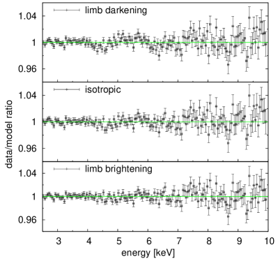
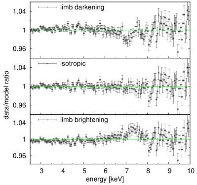
Figure 13: Plots of data/model ratio, where the data are simulated as powerlaw + kyl2cr and the model applied to the data is powerlaw + kyl3cr with a particular analytical approach of the directionality. The default angular momentum value is $a_{\rm f}=0.7$, and the emission angle $\theta_{\rm f}=30^{\circ}$ (left), and $\theta_{\rm f}=60^{\circ}$ (right). These parameters and the normalisation of the reflection component were allowed to vary during the fitting procedure. The plotted results correspond to the terminal values of the parameters obtained during the $\chi^{2}$ minimisation process. Other parameters of the model were kept frozen at their default values: $\Gamma=1.9$, $r_{\rm in}=r_{\rm ms}$, $r_{\rm out}=400$, $q=3$ and normalisation of the power law $K_{\Gamma}=10^{-2}$.

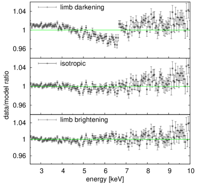
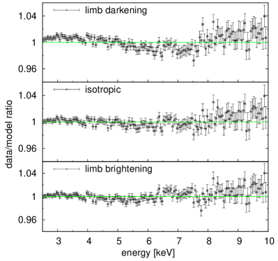
Figure 14: The same plots of data/model ratio, but for $a=0.998$ (left: $\theta_{\rm f}=30^{\circ}$, right: $\theta_{\rm f}=60^{\circ}$).

Figure 15: Results from the test fits with $a_{\rm f}=0.7$ and $\theta_{\rm f}=30\deg$, using the powerlaw + kyl3cr model applied to the data simulated with powerlaw + kyl2cr. Three different profiles of the emission directionality are shown in columns – left: limb brightening, middle: isotropic, right: limb darkening. Top: dependence of the best fit $\chi^{2}$ values on the fiducial spin value. The horizontal (dashed) line represents the 90% confidence level. Bottom: contour graphs of $a$ versus $\theta_{\rm o}$. The contour lines refer to $1$, $2$, and $3$ sigma levels. The position of the minimal value of $\chi^{2}$ is marked with a small cross. The values of $\chi^{2}$ corresponding to the minimum and to the contour levels are shown at the top of each contour graph. The large cross indicates the position of the fiducial values of the angular momentum and the emission angle. Other parameters of the model were kept fixed at default values: $\Gamma=1.9$, $r_{\rm in}=r_{\rm ms}$, $r_{\rm out}=400$, $q=3$ and normalisation of the power law $K_{\Gamma}=10^{-2}$.

Figure 16: The same as in Figure 15, but for $a_{\rm f}=0.7$ and $\theta_{\rm f}=60\deg$.

Figure 17: The same as in Figure 15, but for $a_{\rm f}=0.998$ and $\theta_{\rm f}=30\deg$.

Figure 18: The same as in Figure 15, but for $a_{\rm f}=0.998$ and $\theta_{\rm f}=60\deg$.

	Case 1	Case 2	Case 3
	$a_{\rm f}=0.7$, $\theta_{\rm f}=30^{\circ}$
$a$	$0.60^{+0.02}_{-0.01}$	$0.69^{+0.01}_{-0.01}$	$0.76^{+0.01}_{-0.02}$
$\theta_{\rm{}o}$ [deg]	$29.8^{+0.2}_{-0.3}$	$29.7^{+0.3}_{-0.3}$	$29.6^{+0.3}_{-0.3}$
$\chi^{2}/\nu$	1.33	1.27	1.39
	$a_{\rm f}=0.7$, $\theta_{\rm f}=60^{\circ}$
$a$	$0.65^{+0.03}_{-0.05}$	$0.73^{+0.03}_{-0.04}$	$0.82^{+0.02}_{-0.02}$
$\theta_{\rm{}o}$ [deg]	$60.0^{+0.1}_{-0.2}$	$60.0^{+0.2}_{-0.1}$	$60.3^{+0.1}_{-0.1}$
$\chi^{2}/\nu$	1.87	1.00	1.48
	$a_{\rm f}=0.998$, $\theta_{\rm f}=30^{\circ}$
$a$	$0.956^{+0.005}_{-0.005}$	$1^{+0}_{-1{\rm E}-3}$	$1^{+0}_{-8{\rm E}-5}$
$\theta_{\rm{}o}$ [deg]	$29.9^{+0.3}_{-0.3}$	$29.5^{+0.3}_{-0.3}$	$28.7^{+0.4}_{-0.2}$
$\chi^{2}/\nu$	1.30	1.58	5.08
	$a_{\rm f}=0.998$, $\theta_{\rm f}=60^{\circ}$
$a$	$0.982^{+0.002}_{-0.002}$	$1^{+0}_{-3{\rm E}-4}$	$1^{+0}_{-6{\rm E}-5}$
$\theta_{\rm{}o}$ [deg]	$59.9^{+0.1}_{-0.2}$	$60.1^{+0.1}_{-0.2}$	$60.2^{+0.1}_{-0.2}$
$\chi^{2}/\nu$	1.24	1.02	2.51

Table 2: The best-fit spin and inclination angle values inferred for the three cases of the limb darkening/brightening law in the kyl3cr model. Data were generated using the kyl2cr model. See the main text for details. The quoted errors correspond to the 90$\%$ confidence level.

The results presented in the previous sections show that using different emission directionality approaches leads to a different location of the $\chi^{2}$ minimum in the parameter space. Doubt about the correct prescription for the emission directionality thus brings some non-negligible inaccuracy into the evaluation of the model parameters. The magnitude of this error cannot be easily assessed as a unique number because other parameters are also involved.

A possible way to tackle the problem is to derive the intrinsic spectrum from self-consistent numerical computations. This has the potential of removing the uncertainty about the emission directionality (although, to a certain degree this uncertainty is only moved to a different level of the underlying model assumptions). In this section, we present such results from modelling the artificial data generated by numerical simulations, i.e. independently of an analytical approximation of the emission directionality presented in the previous sections.

Let us first remind the reader that the orbital speed within the inner $\lesssim 10r_{\rm g}$ reaches a considerable fraction of the speed of light (Fig. 1). Beaming, aberration, and the light-bending all affect the emitted photons very significantly in this region. Less energetic photons come from the outer parts where the motion slows down and the relativistic effects are of diminished importance. This reasoning suggests that the analysis of the previous section may be inaccurate because the adopted analytical approximations (8) neglect any dependence on energy and distance.

We applied the Monte-Carlo radiative transfer code NOAR (see Section 5 in Dumont et al. 2000) for the case of “cold” reflection, i.e. for neutral or weakly-ionised matter. The NOAR code computes absorption cross sections in each layer. Free-free absorption and the recombination continua of hydrogen- and helium- like ions are taken into account, as well as the direct and inverse Compton scattering. The NOAR code enables us to obtain the angle-dependent intensity for the reprocessed emission. The cold reflection case serves as a reference point that we will later, in a follow-up paper, compare against the models involving stronger irradiation and higher ionisation of the disc medium.

The directional distribution of the intrinsic emissivity of the reprocessing model is shown in Fig. 4 (right panel). The continuum photon index $\Gamma=1.9$ is considered and the energies are integrated over the $2$–$100$ keV range. Although the results of the radiation transfer computations do show the limb-brightening effect, it is a rather mild one, and not as strong as the Case 1. In the same plot we also show the angular profile of the emissivity distribution in different energy ranges: (i) 2–6 keV (i.e. below the iron K$\alpha$ line rest energy); (ii) 6–15 keV (including the iron K$\alpha$ line); (iii) 15–100 keV (including the ‘Compton hump’). We notice that the energy integrated profile is dominated by the contribution from the Compton hump, where much of the emerging flux originates. However, all of the energy sub-ranges indicate the limb-brightening effect, albeit with slightly different prominence.

We implemented the numerical results of NOAR modelling of a reflected radiation from a cold disc as kyl2cr in the ky collection of models. Furthermore, we produced an averaged model, kyl3cr, by integrating kyl2cr tables over all angles. Therefore, kyl3cr lacks information about the detailed angular distribution of the intrinsic local emission from the disc surface. On the other hand, it has the advantage of increased computational speed and the results are adequate if the emission is locally isotropic. Furthermore, kyl3cr can be a posteriori equipped with an analytical prescription for the angular dependence (Cases 1–3 in eq. 8), which brings the angular resolution back into consideration. This approach allows us to switch between the three prescriptions for comparison and rapid evaluation.

In order to constrain the feasibility of the aforementioned approaches, we generated the artificial data using the powerlaw + kyl2cr model. The parameters of the model are: photon index of the power law $\Gamma=1.9$ and its normalisation $K_{\Gamma}=0.01$, spin of the black hole $a$, inclination angle $\theta_{\rm o}$, the inner and outer radii of the disc $r_{\rm in}=r_{\rm ms}$ and $r_{\rm out}=400$, the index of the radial dependence of the emissivity $q=3$, and the normalisation of the reflection component $K_{\rm kyl2cr}=0.1$. We simulated the data for two different values of the spin, $a=0.7$ and $a=0.998$, and for inclination angles $\theta_{\rm o}=30^{\circ}$ and $\theta_{\rm o}=60^{\circ}$. The simulated flux of the primary power law component is the same as in the previous section. However, now an important fraction of the primary radiation is reflected from the disc. The total flux depends on the extension of the disc and its inclination. Its value is $4.9-5.6\times 10^{-11}$ erg cm^-2 s^-1 for our choice of the parameters.

As a next step, we replaced kyl2cr by kyl3cr and searched back for the best-fit results using the latter model. In this way, using kyl3cr we obtained the values of the spin and the inclination angle for different directionalities. The fitting results are summarised in Table 2. Besides the spin and the inclination angle, only normalisation of the reflection component was allowed to vary during the fitting procedure. The remaining parameters of the model were kept frozen at their default values.

The resulting data/model ratios are shown in Figures 13 and 14. For $a=0.7$ and $\theta_{\rm o}=30^{\circ}$ the graphs look very similar in all three cases. However, the inferred spin value differs from the fiducial value with which the test data were originally created. The dependence of the best-fit $\chi^{2}$ statistic on the spin and the corresponding graphs of the confidence contours for spin versus inclination angle are shown in Figures 15–18, again for the three cases of angular directionality. These figures confirm that for the limb-brightening profile the inferred spin value comes out somewhat lower than the correct value, whereas it is higher if the limb-darkening profile is assumed.

In each of the three cases the error of the resulting $a$ determination depends on the inclination angle and the spin itself. However, we find that the isotropic directionality reproduces our data to the best precision. The limb darkening profile is not accurate at higher values of the spin, such as $a=0.998$, when the resulting $\chi^{2}/\nu$ value even exceeds $2$. The limb darkening profile is characterised by an enhanced blue peak of the line while the height of the red peak is reduced (see Figs. 5–6). Consequently, the model profile is too steep to fit the data. This is clearly visible in the data/model ratio plots for $a=0.998$ shown in Figures 14. The flux is underestimated by the model below a mean energy value $E_{\rm mean}$ of the line (for $a=0.998$ and $i=30$ deg $E_{\rm mean}\approx 5$ keV) and overestimated above $E_{\rm mean}$. This fact leads to a noticeable jump in the data/model ratio plot. Only the $q$ parameter can mimic this limitation and suit the data by increasing its value. It could be the case of the analysis of the MCG–6-30-15 data in the previous section.

A noteworthy result appears in comparing of the contours produced by the model with limb brightening and limb darkening for $a=0.7$ and $i=60$ deg (Fig. 16). Although the former model (limb brightening) gives a statistically worse fit with $\chi^{2}/\nu=1.87$ than the limb darkening case ($\chi^{2}/\nu=1.48$), the inferred values of the spin and the inclination angle are consistent with the fiducial values within the $3\sigma$ level. On the other hand, the spin value inferred from the limb darkening model is far from the fiducial (i.e., the correct) value.

4 Discussion

We investigated whether the spin measurements of accreting black holes are affected by the uncertainty of the angular emissivity law, ${\cal M}(\mu_{\rm e},r_{\rm e},E_{\rm e})$, in the relativistically broadened iron K$\alpha$ line models. We employed three different approximations of the angular profiles, representing limb brightening, isotropic and limb darkening emission profiles. For the radius-integrated line profile of the disc emission, and especially for higher values of the spin, the broadened line has a triangle-like profile. The differences among the considered profiles concern mainly the width of the line’s red wing. However, the height of the individual peaks, also affected by the emission directionality, is important for the case of an orbiting spot (or a narrow ring), which produce a characteristic double-horn profile.

We reanalysed an XMM-Newton observation of MCG–6-30-15 to study the emission directionality effect on the broad iron line, as measured by current X-ray instruments. We showed the graphs of $\chi^{2}$ values as a function of spin for different cases of directionality. We can conclude that the limb darkening law favors higher values of spin and/or steeper radial dependence of the line emissivity; vice versa for the limb brightening profile. Both effects are comprehensible after examining the left panel of Fig. 5. The limb darkening profile exhibits a deficit of flux in the red wing compared with the limb brightening profile. Both higher spin value and steeper radial profile of the intensity can compensate for this deficit.

The higher spin value has the effect of shifting the inferred position of the marginally stable orbit (ISCO) closer to the black hole, in accordance with eq. (4). Consequently, the accretion disc is extended closer to the black hole. The radiation comes from shorter radii and it is affected by the extreme gravitational redshift. Hence, the contribution to the red wing of the total disc line profile is enhanced. Naturally, these considerations are based on the assumption that the inner edge of the line emitting region coincides with the ISCO. Likewise, the steeper radial dependence of the emissivity means that more radiation comes from the inner parts of the accretion disc than from the outer parts, and this produces a similar effect to decreasing the inner edge radius. With the limb brightening law the above-given considerations work the other way around.

We further simulated the data with the powerlaw + kyrline model. The simple model allows us to keep better control over the parameters and to evaluate the differences in the spin determination. We used one of the preliminary response matrices for the IXO mission and we chose the flux at a level similar to bright Seyfert 1 galaxies observable by current X-ray satellites (Nandra et al. 2007). The simulations with the kyrline model confirm that the measurements would overestimate the spin for the limb darkening profile and, vice versa, they tend to the lower spin values for the limb brightening profile.

Although the interdependence of the model parameters is essential and it is not possible to give the result of our analysis in terms of a single number, one can very roughly estimate that the uncertainties in the angular distribution of the disc emission will produce an uncertainty of the inferred inner disc radius of about $20$% for the high quality data by IXO. We consider this value as realistic.

In the next step, we applied the NOAR radiation transfer code to achieve a self-consistent simulation of the outgoing spectrum without imposing an ad hoc formula for the emission angular distribution. In this paper we assumed a cold isotropically illuminated disc with a constant density atmosphere. We created new models for the KY suite, kyl2cr and kyl3cr. The results of NOAR computations of the cold disc are implemented in the kyl2cr model, while the kyl3cr model uses the angle-integrated tables over the entire range of emission directions. This enables us to include, a posteriori, the analytical formulae for directionality and check how precisely they reproduce the original angle-resolved calculations. We simulated the data using the preliminary IXO response matrix and we analysed them using the powerlaw + kyl2cr model. Then we used the kyl3cr model to test the analytical directionality approaches on these artificial data.

We found that, for $a=0.998$, none of the three assumed cases of the directionality profile covered the fiducial values for the spin and the inclination angle within the $3\sigma$ contour line (see Figs. 17–18). The suitability of the particular directionality prescription depends on the fiducial values of the spin and the inclination angle. The limb brightening profile successfully minimises the $\chi^{2}$ values for $a=0.998$ and $i=30$ deg, but for $a=0.7$ and $i=60$ deg it gives the worst fit of all studied cases of the directionality laws.

On the whole, we found that the isotropic angular dependence of the emission intensity fits best. Especially for higher values of the black hole spin, the model with the limb darkening profile was not able to reproduce the data: the best fit $\chi^{2}/\nu$ value exceeds $5$ for $a=0.998$ and $i=30$ deg, which means a more than three times worse fit than using isotropic or limb brightening directionality. The inclination angle was underestimated by more than $1$ deg.

This is an important result because much of the recent work on the iron lines, both in AGN and black hole binaries, has revealed a significant relativistic broadening near rapidly rotating central black holes (Miller 2007). In some of these works, the limb darkening law was employed and different options were not tested. The modelled broad lines are typically characterised by a steep power law in the radial part of the intensity across the inner region of the accretion disc, as in the mentioned MCG–6-30-15 observation. This behaviour has been interpreted as a case of a highly spinning compact source where the black hole rotational energy is electromagnetically extracted (Wilms et al. 2001). We conclude that the significant steepness of the radial part of the intensity also persists in our analysis, however, the exact values depend partly on the assumed angular distribution of the emissivity of the reflected radiation.

It should be noted that, in reality, the angular distribution of the disc emission is significantly influenced by the vertical structure of the accretion disc. However, our comprehension of accretion disc physics is still evolving. In recent years, several detailed models have been developed for irradiated black hole accretion discs in hydrostatic equilibrium (see e.g. Nayakshin 2000; Ballantyne et al. 2001; Różańska et al. 2002). These models combine radiative transfer simulations with calculations of the hydrostatic balance in the stratified disc medium. Aside from reprocessing spectra, the models provide solutions for the vertical disc profile of the density, temperature, and ionisation fractions. In Goosmann et al. (2007) the effects of general relativity and advection on the disc medium were added.

In Nayakshin (2000), Goosmann et al. (2007), and Różańska & Madej (2008) the reprocessed spectra are evaluated at different local emission angles. The shape and normalisation of these spectra depend on various model assumptions. Until we know in more detail how accretion discs work, it is hard to choose which is the “correct” reprocessing model. One could always argue that more physical processes and properties should be included in the radiative transfer simulations, such as the impact of magnetic fields, macroscopic turbulence, or different chemical compositions of the medium. Using the above-mentioned models for an accretion disc in hydrostatic equilibrium may then easily become computationally intense.

For the practical purpose of data analysis, however, the computation of large model grids is necessary, which requires sufficiently fast methods. This is why simple constant density models are most often used to analyse the observational data. In fact, Ballantyne et al. (2001) have shown that their reprocessing spectra for a stratified disc medium in hydrostatic equilibrium can be satisfactorily represented by spectra that are computed for irradiated constant density slabs. Therefore, we include in our present analysis the angular emissivity obtained from the modelling of neutral reprocessing in a constant density slab. For the purpose of this paper we have not discussed in any further detail the dependence on the ionisation parameter, which we expect to be rather important. It will be addressed in a future article.

We emphasise that the main strategy of the present paper is not intended to find the “correct” angular emissivity, as this is still beyond our computational abilities and understanding of all the physical processes shaping the accretion flow. Instead, we examined the three different prototypical dependencies which are mutually disparate (i.e., the limb-darkening, isotropic, and limb-brightening cases), applied in current data analysis, and which presumably reflect the range of possibilities. By including these different cases we mimic various uncertainties, such as those in the vertical stratification, and we estimate the expected error that these uncertainties can produce in the spin determinations. Further detailed computations of reprocessing models and the angular emissivity are needed in the future in order to understand its role in different spectral states of accreting black holes.

5 Conclusions

Black hole spin measurements using X-ray spectroscopy of relativistically broadened lines depend on the definition employed of the angular distribution of the disc emission. We studied three cases of the directionality profile - limb brightening, isotropic and limb darkening.

We found that isotropic directionality is consistent with our radiation transfer computations of the reflection spectra of an irradiated cold disc. This eliminates any need for ad hoc approximations to the limb-darkening profile. Using an improper directionality profile could impact on the other parameters inferred for the relativistic broad line model. Especially for the often used case of limb darkening, the radial steepness can interfere with the line parameters of the best-fit model by enhancing the red wing of the line.

Uncertainties in the precise position of the inner edge can further increase the error of the spin determination; however, it appears that the expected magnitude of these errors does not prevent us from setting interesting and realistic constraints on the spin parameter. Our present treatment of the problem is incomplete by neglecting the magnetohydrodynamical effects and their influence on the ISCO location. Future improvements in our theoretical understanding of the inner edge location are highly desirable and will help to improve the confidence in the determination of the model parameters.

We verified our conclusions by comparing them with the results based on an XMM-Newton long observation of MCG–6-30-15, and we found them to be broadly consistent. The expected improvement of sensitivity of the future IXO mission will significantly advance the reliability of the spin determinations.