Correlated hopping of bosonic atoms induced by optical lattices

Abstract

In this work we analyze a particular setup with ultracold atoms trapped in state-dependent lattices. We show that any asymmetry in the contact interaction translates into one of two classes of correlated hopping. After deriving the effective lattice Hamiltonian for the atoms, we obtain analytically and numerically the different phases and quantum phase transitions. We find for weak correlated hopping both Mott insulators and charge density waves, while for stronger correlated hopping the system transitions into a pair superfluid. We demonstrate that this phase exists for a wide range of interaction asymmetries and has interesting correlation properties that differentiate it from an ordinary atomic Bose-Einstein condensate.

1 Introduction

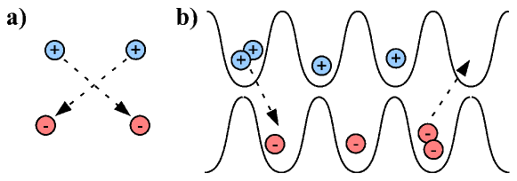
Figure 1: (a) Two atoms in state $\left|{+}\right\rangle$ collide and flip state in free space. (b) When these atoms are confined in a state-dependent optical lattice, their change of state must be accompanied by a tunneling event to a neighboring site. This leads to correlated hopping of atoms through the lattice.

Ultracold neutral atoms are a wonderful tool to study many-body physics and strong correlation effects. Since the achievement of Bose-Einstein condensation in alkali atoms [1, 2, 3], we have been witnesses of two major breakthroughs. One is the cooling of fermionic atoms and the study of Cooper pairing and the BCS to BEC transition [4, 5, 6]. The other one is the implementation of lattice Hamiltonians using bosonic [7, 8] and fermionic atoms in off-resonance optical lattices. Contemporary and supported by these experimental achievements, a plethora of theoretical papers has consolidated ultracold atoms as an ideal system for quantum simulations. The goal is two-fold: AMO is now capable of implementing known Hamiltonians which could describe real systems in Condensed Matter Physics, such as Hubbard models [8] and spin Hamiltonians [9, 10]; but it is also possible to study new physical effects, such as the quantum Hall effect with bosons [11] and lattice gauge theories [12, 13].

In this work we deepen and expand the ideas presented in [14], where we introduced a novel mechanism for pairing based on transport–inducing collisions. As illustrated in Fig. 1, when atoms collide they can mutate their internal state. If the atoms are placed in a state-dependent optical lattice, whenever such a collision happens the pair of atoms must tunnel to a different site associated to their new state. For deep enough lattices, as in the Mott insulator experiments [7], this coordinated jump of pairs of particles can be the dominant process and the ensemble may become a superfluid of pairs.

The focus of this work is to develop these ideas for all possible interaction asymmetries that can happen in experiments with bosonic atoms in two internal states, where the scattering lengths among different states can be different, $(g_{\uparrow\uparrow}\neq g_{\downarrow\downarrow})$ [15]. We want to understand the different types of correlated hopping that appear when we move beyond the limited type of interactions considered in Ref. [14]. We will better study the resulting phases and phase transitions, using different analytical and numerical tools that describe the many body states, and evolving from few particles to more realistic simulations. The main results will be to show that when one considers more general asymmetries, a new type of correlated hopping appears, but that both the previous [14] and the newly found two–body terms cooperate in creating a superfluid state with pair correlations. Indeed, this new state will also be shown to be more than just a condensate of pairs, based on analytical and numerical studies.

Correlated hopping is not a new idea. It appears naturally in fermionic tight-binding models, where it has been used to describe mixed valence solids [16] and, given that they are able to mimic the attractive interactions between electrons, also high-$T_{c}$ superconductors [17, 18, 19, 20, 21, 22]. In most of these works, the correlated hopping appears in the form $n_{i}a^{\dagger}_{j}a_{k},$ indicating that the environment can influence the motion of a particle. This would seem substantially different from correlated motion of pairs of fermions. Nevertheless, even this more elaborate form of correlated hopping has been shown to lead to the formation of bound electron pairs [20, 19] and it has been put forward as a possible explanation for high $T_{c}$ superconductivity [23, 24].

This work is organized as follows. In Sec. 2 we introduce our model of correlated hopping (1), qualitatively discussing how it originates and what are the quantum phases that we expect it to develop. We present a possible implementation of this model which is based on optical superlattices and atoms with asymmetric interactions. Sec. 3 includes exact diagonalizations for a small number of atoms and sites. These calculations reveal the existence of insulating and coherent regimes, as well as pairing, and will be the basis for later analysis. In Sec. 4 we study the many-body physics of larger lattices with correlated hopping, using a variety of techniques: starting with insulating regime and following with the implementation of perturbation theory and the quantum rotor model. These methods suggest a number of possible phases, including a Mott insulator, a pair superfluid, a normal superfluid and a charge density wave state, and we estimate the parameters for which these phases appear. In Sec. 5 we develop two numerical methods to study our system, a Gutzwiller ansatz and an infinite Matrix Product State method. With these simulations we confirm the above mentioned phases and locate the quantum phase transitions, which are found to be of second order. Finally, in Sec. 6 we suggest some currently available experimental methods to detect and characterize these phases.

2 Correlated hopping model

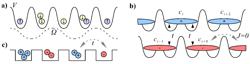
Figure 2: (a) Atoms in two internal states $\uparrow$ and $\downarrow$ are trapped in an optical lattice and coupled by a Raman laser with Rabi frequency $\Omega$. (b) That setup is equivalent to two displaced superlattices for the dressed states $\left|{\pm}\right\rangle\sim\left|{\uparrow}\right\rangle\pm\left|{\downarrow}\right\rangle$. (c) When asymmetric contact interactions are considered and the hopping between superlattice cells neglected, the whole system behaves effectively as a $1$D array of alternating $\left|{+}\right\rangle$ and $\left|{-}\right\rangle$ sites, with transitions of tunneling amplitude $t$ between them.

We suggested in Ref. [14] that the combination of atomic collisions with optical superlattices can be used to induce correlated hopping. The basic idea is shown in Fig. 2b, where atoms are trapped in two orthogonal states called $(+)$ and $(-).$ The interaction terms change the state of the atoms, forcing them to hop to a different superlattice every time they collide. In this sense, interactions are responsible for transport.

In this section we introduce the most general model of correlated hopping that can be produced by such means with two–states bosons. This model is presented in the following subsection, where we explain qualitatively the role of each Hamiltonian term. Later on, in Sec. 2.2, we establish the connection between the parameters of this model and the underlying atomic model. This is the foundation for the subsequent analytical and numerical studies.

2.1 Lattice Hamiltonian

In this work we study the ground state properties of a very general Hamiltonian that contains different kinds of correlated hopping. More precisely, the model will be

$$H = \sum_{i}\bigg{\{}\frac{U}{4}:(n_{i}+n_{i+1})^{2}:+~{}V~{}n_{i}n_{i+1}-t~{}(c_{i}^{\dagger 2}c_{i+1}^{2}+\mathrm{H.c.})$$ (1)

$$~{}~{}~{}~{}~{}~{}~{}-j[(n_{i}-1)c^{\dagger}_{i}(c_{i-1}+c_{i+1})+\mathrm{H.c.}]\bigg{\}}.$$

Here, $c_{i}^{\dagger}$ and $c_{i}$ are bosonic operators that create and anihilate atoms according to the site numbering from Fig. 2b-c, and the colons $:A_{i}B_{j}:$ denote normal ordering of operators $A_{i}$ and $B_{j}.$

Let us qualitatively explain the roles of the different terms in Eq. (1). The first and second terms, $U$ and $V,$ are related to on-site and next-neighbor interactions. When these terms are dominant, we expect the atoms in the lattice form an insulator. Such a phase is characterized by atoms being completely localized to lattice sites, having well-defined occupation numbers, the absence of macroscopic coherence and a gapped energy spectrum. Whether this insulating state is itself dominated by strong on–site interactions $U$ or by nearest–neighbor repulsion/attraction $V$ will decide whether it presents an uniform density, a Mott insulator (MI), or a periodic density pattern, a charge density wave (CDW), respectively.

The third term is the key feature of our model. It describes the tunneling of pairs between neighboring lattice sites, with amplitude $t.$ Given $U,V,j=0,$ we expect the atoms to travel along the lattice in pairs forming what we call a pair superfluid (PSF). These pairs will be completely delocalized, establishing long range coherence along the lattice. The observable $\langle a^{2}\rangle$ would be the figure of merit describing this kind of delocalization, while a vanishing $\langle a\rangle$ indicates the absence of the single-particle correlations appearing in a normal superfluid. Furthermore, we expect this phase to have a critical velocity, similar to that of an atomic condensate, and the energy spectrum should be gapless.

Unlike in Ref. [14], when one considers the most general kind of atomic interaction, a second kind of correlated hopping appears, described by the last term in Eq. (1). Here, individual atoms will hop only if there is already a particle in the site they go to ($c_{i}^{\dagger}c_{j}(n_{i}-1)$) or leave at least a particle behind ($(n_{i}-1)c_{j}c_{i}^{\dagger}$). One might be induced to think that this term is equivalent to single–particle hopping with a strength that depends on the average density, thus giving rise to a single-particle superfluid (SF) phase. However, this does not seem to be the case. We will show that the correlated hopping $j$ generates a mixed phase which contains features of both the ordinary BEC and the PSF created by $t.$

2.2 Relation to atomic parameters

We now establish the relation between the model in Eq. (1) and the dynamics of atoms in an optical superlattice. The actual setup we have in mind is shown in Fig. (2)a-b and described in more detail in A.1. It consists on a three–dimensional lattice that is strongly confining along the $Y$ and $Z$ directions, creating isolated tubes. On top of this, we create an optical superlattice acting along the $X$ direction [14]. This superlattice traps atoms in the dressed states $\left|{+}\right\rangle$ and $\left|{-}\right\rangle,$ while the atomic interaction is diagonal in the basis of bare states $\left|{\uparrow}\right\rangle$ and $\left|{\downarrow}\right\rangle.$ The interaction will be described by a contact potential and parameterized by some real constants $g_{\alpha\beta}$

$$H_{\mathrm{int}} = \sum_{\alpha,\beta=\uparrow,\downarrow}\frac{g_{\alpha\beta}}{2}\int\psi_{\alpha}^{\dagger}(x)\psi_{\beta}^{\dagger}(x)\psi_{\beta}(x)\psi_{\alpha}(x)dx$$

$$= \sum_{\alpha,\beta=\uparrow,\downarrow}\frac{g_{\alpha\beta}}{2}\int{:\rho_{\alpha}(x)\rho_{\beta}(x):}\,dx$$

These interaction constants are functions of the s–wave one–dimensional scattering lengths between different species $g_{\alpha\beta}=4\pi\hbar^{2}a^{(1D)}_{\alpha\beta}/m.$ In general, the interaction strengths among different atomic components are different from each other, a situation that can be enhanced with Feshbach resonances. We will use a parameterization

$$g_{\uparrow\downarrow}=g_{0}+g_{1}=g_{\downarrow\uparrow},\quad g_{\uparrow\uparrow}=g_{0}+g_{2},\quad g_{\downarrow\downarrow}=g_{0}-g_{2},$$ (3)

that makes the symmetries more explicit

$$H_{\mathrm{int}} = \frac{g_{0}}{2}\int{:(\rho_{\uparrow}(x)+\rho_{\downarrow}(x))^{2}:}\,dx+g_{1}\int{:\rho_{\uparrow}(x)\rho_{\downarrow}(x):}\,dx$$ (4)

$$+\frac{g_{2}}{2}\int{:\rho_{\uparrow}(x)^{2}-\rho_{\downarrow}(x)^{2}:}\,dx$$

The total Hamiltonian combines the previous interaction with the kinetic energy and the trapping potential for one particle

$$H_{\mathrm{1}}=\sum_{s=\pm}\int\psi^{\dagger}_{s}(x)\left[-\frac{\hbar^{2}}{2m}\nabla^{2}+V_{s}(x)\right]\psi_{s}(x)dx,$$ (5)

which is written in a different basis

$$\psi_{\uparrow}(x)=\frac{1}{\sqrt{2}}(\psi_{+}+\psi_{-}),\quad\psi_{\downarrow}(x)=\frac{1}{\sqrt{2}}(\psi_{+}-\psi_{-}).$$ (6)

Since the superlattice potential $V_{\pm}(x)$ is the dominant term, we may approximate the bosonic fields as linear combinations of the Wannier modes in this superlattice and in the dressed state basis, a process detailed in A. Note that out of all the terms in the interaction Hamiltonian (4), only the first one is insensitive to the state of the atoms. This is important because the asymmetries $g_{1}$ and $g_{2},$ when expressed in the dressed basis, produce terms that change the state of the atoms during a collision. Once we introduce the effective interaction constants in the lattice

$$U_{i}=g_{i}\int|w(x)|^{4}dx\quad\quad\mathrm{for}~{}i=0,1,2$$ (7)

where $w(x)$ is the single site Wannier wavefunction, we arrive to the effective Hamiltonian in Eq. (1) with parameters $U,V,t$ and $j$ that relate to the microscopic model as follows

$$U=\frac{2U_{0}+U_{1}}{4},~{}~{}V=-\frac{U_{1}}{8},~{}~{}t=\frac{U_{1}}{16}~{}~{}\mathrm{and}~{}~{}j=\frac{U_{2}}{8}.$$ (8)

Unlike in the specific case of Ref. [14], the most general situation contains not only two-body correlated hopping $t,$ but also the terms proportional to $j.$

3 Preliminary analysis

In this section we study the eigenstates of Hamiltonian (1) for systems that we can diagonalize exactly. The goals are to characterize the effect of the different interaction and hopping terms, as well as to understand the structure of the ground state wavefunction. Although we are limited to a small number of particles, the following examples provide enough evidence of the roles of correlated hopping, nearest neighbor repulsion and the utility of different correlators to characterize the states.

3.1 A two-sites example

Let us take the simplest interesting case: four particles in two sites. We write the Hamiltonian in the basis $\{\left|{40}\right\rangle,\left|{22}\right\rangle,\left|{04}\right\rangle,\left|{31}\right\rangle,\left|{13}\right\rangle\},$ where the notation $\left|{n_{1}n_{2}}\right\rangle$ stands for $n_{1}$ particles in the first site and $n_{2}$ in the second and we restrict to $n_{1}+n_{2}=4,$

$$~{}~{}~{}~{}~{}H_{\mathrm{4/2}}=\left(\begin{array}[]{ccccc}0&-4\sqrt{6}t&0&-12j&0\\ -4\sqrt{6}t&8V&-4\sqrt{6}t&-6\sqrt{6}j&-6\sqrt{6}j\\ 0&-4\sqrt{6}t&0&0&-12j\\ -12j&-6\sqrt{6}j&0&6V&-12t\\ 0&-6\sqrt{6}j&-12j&-12t&6V\\ \end{array}\right)+6U.$$ (9)

Notice that in this particular case, $U$ gives rise to a global energy shift and does not affect the different eigenstates. This is consistent with later studies where we will see that on-site interactions just add a global, density dependent contribution to the energy. To better understand the role of the remaining terms, we will consider separately three limiting cases, two of superfluid nature and an insulating one.

Limit $j\neq 0,$ $t=V=0,$ single-particle delocalization.

In this case we take for simplicity $V=0$ and diagonalize Eq. 9, finding the normalized ground state

$$\left|{\psi_{0,t=0}}\right\rangle=\frac{1}{4}\left|{40}\right\rangle+\frac{1}{2}\sqrt{\frac{3}{2}}\left|{22}\right\rangle+\frac{1}{4}\left|{04}\right\rangle+\frac{1}{2}\left|{31}\right\rangle+\frac{1}{2}\left|{13}\right\rangle.$$ (10)

Note that this state is exactly a BEC of $4$ particles spread over two sites

$$\left|{\psi_{BEC}(4)}\right\rangle=\frac{1}{\sqrt{4!}}\left(\frac{1}{\sqrt{2}}\sum_{i=1}^{2}c_{i}^{\dagger}\right)^{4}\left|{00}\right\rangle.$$ (11)

This suggests that, at least in this small example, the correlated hopping proportional to $j$ is equivalent to the single-particle hopping in the ordinary Bose-Hubbard model, giving rise to the delocalization of individual particles. However, as it will become evident later on, for larger systems and more particles this interpretation is wrong.

Limit $j=0,$ $t\gg|V|,$ pair delocalization.

In the presence of two particle hopping, the lowest energy state has the form

$$\left|{\psi_{0,j=0}}\right\rangle=c_{40}(t,V)\left|{40}\right\rangle+c_{22}(t,V)\left|{22}\right\rangle+c_{04}(t,V)\left|{04}\right\rangle$$ (12)

with coefficients

$$c_{22}(t,V)\propto-V+\sqrt{12t^{2}+V^{2}},$$

$$c_{40}(t,V)=c_{04}(t,V)\propto\sqrt{6}t.$$

In particular, for dominant pair hopping $t\gg|V|$ this is a state of delocalized pairs

$$\left|{\psi}\right\rangle=\frac{1}{2}\left|{40}\right\rangle+\frac{1}{\sqrt{2}}\left|{22}\right\rangle+\frac{1}{2}\left|{04}\right\rangle.$$ (13)

Observe that this wavefunction is not equivalent to what one would naïvely understand as a “pair condensate” from analogy with the single-particle case

$$\left|{\psi}\right\rangle\neq\left(\sum_{i=1}^{2}c_{i}^{\dagger 2}\right)^{2}\left|{\mathrm{vac}}\right\rangle\sim\sqrt{\frac{3}{8}}\left|{40}\right\rangle+\frac{1}{2}\left|{22}\right\rangle+\sqrt{\frac{3}{8}}\left|{04}\right\rangle.$$ (14)

Instead the previous wavefunction is isomorphic to the BEC of two bosons

$$\left|{\psi_{BEC}(2)}\right\rangle=\frac{1}{2}\left|{20}\right\rangle+\frac{1}{\sqrt{2}}\left|{11}\right\rangle+\frac{1}{2}\left|{02}\right\rangle$$ (15)

under the replacement of each boson with two atoms. It is also interesting to remark that $\psi_{BEC}(2)$ has larger pair-correlations than the state in Eq. (14).

Limit $|V|\to\infty,$ an insulator.

Reusing the previous wavefunction (12) and taking the limit of dominant nearest-neighbor interaction $V,$ we obtain two possible states. For strong repulsion $V\to+\infty,$ states $\left|{40}\right\rangle$ and $\left|{04}\right\rangle$ are favored, forming a charge density wave (CDW) with partial filling $\left|{\psi_{CDW}}\right\rangle\propto\left|{40}\right\rangle+\left|{04}\right\rangle.$ On the other hand, for strong nearest-neighbor attractions $V\to-\infty,$ the particles are evenly distributed forming a Mott insulator $\left|{22}\right\rangle.$

3.2 Superfluidity of pairs

We have seen that four particles in a two-sites lattice recreate the exact wavefunction of an ordinary BEC under the replacement of single bosons with pairs. We can test this idea for slightly bigger lattices, diagonalizing numerically the Hamiltonian which only contains the pair hopping term ($t\neq 0,~{}V,U,j=0$). The resulting wavefunctions are compared side by side with the BEC-like ansatz we mentioned. In the case of two particles we get indeed the expected result

$$\left|{\psi_{2}^{g.s.}}\right\rangle = \left|{\psi_{2}^{ideal}}\right\rangle\sim\sum_{i=1}^{L}a^{\dagger 2}_{i}\left|\mathrm{vac}\right\rangle,$$

whereas for $4$ particles in $5$ sites

$$\left|{\psi_{4}^{g.s.}}\right\rangle = c_{1}\big{(}\left|{40000}\right\rangle+\left|{04000}\right\rangle+\left|{00400}\right\rangle+\left|{00040}\right\rangle+\left|{00004}\right\rangle\big{)}$$

$$+c_{2}\big{(}\left|{22000}\right\rangle+\left|{02200}\right\rangle+\left|{00220}\right\rangle+\left|{00022}\right\rangle+\left|{20002}\right\rangle\big{)}$$

$$+c_{3}\big{(}\left|{20200}\right\rangle+\left|{20020}\right\rangle+\left|{02020}\right\rangle+\left|{02002}\right\rangle+\left|{00202}\right\rangle\big{)},$$

we find a disagreement between the ideal case of a BEC-like state with coefficients $c_{1}=1/5,c_{2}=c_{3}=\sqrt{2}/5,$ and the exact diagonalization with $c_{1}\sim 0.2735,$ $c_{2}\sim 0.3073$ and $c_{3}\sim 0.1754.$ We observe that when compared to the ideal BEC, our paired state breaks the translational symmetry, revealing an effective attraction between different pairs, that favors their clustering.

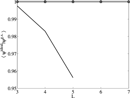
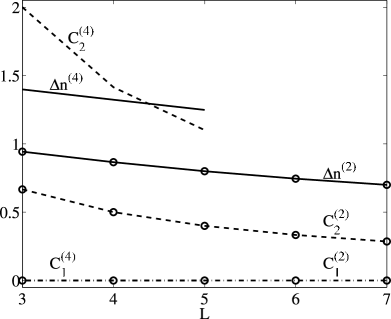
Figure 3: (left) Fidelity between the ground state of the Hamiltonian and the ideal PSF for the case of 2 particles (line with circles) and 4 (no markers). (right) Particle fluctuation (solid), one-body correlator (dot-dash) and two-body correlator (dash) for the case of 2 particles (circle) and 4 (no markers) using the ground state of the Hamiltonian.

In Fig. 3 we plot the projection between these states, namely the solution of Eq. 1 with only $t\neq 0$ and the ideal superfluid of pairs. In the nearby plot we also analyze two relevant correlators that will be also used later on in the manuscript, namely, a single-particle coherence

$$C_{\Delta}^{1}=\frac{1}{L}\sum_{i}\left\langle a^{\dagger}_{i+\Delta}a_{i}\right\rangle$$ (16)

and the pair correlator

$$C_{\Delta}^{2}=\frac{1}{L}\sum_{i}\left\langle a^{\dagger 2}_{i+\Delta}a_{i}^{2}\right\rangle.$$ (17)

As it is evident from the wavefunction and from the plots, there is no single-particle coherence or delocalization because particles move in pairs. Hence, $C^{1}_{\Delta}\sim\delta_{\Delta 0}.$ The other correlator, $C^{2}_{\Delta},$ which we identify with the delocalization of pairs is rather large and it only decreases with increasing the lattice size because the total pair density becomes smaller.

4 Analytical methods

We now study the many-body physics of our model for a much larger number of particles using exact analytical methods. We begin with the regime in which the interaction terms $U$ and $V$ dominate, obtaining the different insulator phases on the $j,t=0$ plane. Then, using perturbation theory, we compute the phase boundaries of these insulating regions for growing $j$ and $t.$ Finally, we study the properties of the ground state and its excitations in the superfluid phase, with $j=0$ and dominating $t,$ proving indeed that this region describes a superfluid of pairs.

4.1 No hopping limit: insulating phases

To analyze the phase diagram it is convenient to work in the grand-canonical picture, in which the occupation is determined by the chemical potential $\mu.$ In this picture the ground state is determined by minimizing the free energy

$$F=H-\mu N,$$ (18)

where $N=\sum_{k}n_{k}$ is the total number of particles, including both states $\left|{+}\right\rangle$ and $\left|{-}\right\rangle.$ The free energy has a very simple form in the absence of tunneling

$$F = \sum_{k}\left[\frac{U}{4}:(n_{k}+n_{k+1})^{2}:+Vn_{k}n_{k+1}-\mu n_{k}\right]$$

$$= \sum_{k}\left[\frac{U}{4}(n_{k}+n_{k+1})^{2}+Vn_{k}n_{k+1}-\left(\frac{2\mu+U}{4}\right)(n_{k}+n_{k+1})\right].$$

This function is defined over positive occupation numbers $n_{k}\in\{0,1,2,\ldots\}.$ A discrete minimization will determine the different insulating phases and the regions where the system is stable against collapse.

For a translational invariant system with periodic boundary conditions, all solutions can be characterized as a function of two integers ${\vec{x}}^{t}=(n,m),$ representing the occupations of even $n_{2k}=n$ and odd sites $n_{2k+1}=m.$ The optimization begins by noticing that the bond energy of two sites has a quadratic form

$$\varepsilon(\vec{x}) = {\vec{x}}^{t}\left(\begin{array}[]{cc}U/4&(U+2V)/4\\ (U+2V)/4&U/4\end{array}\right)\vec{x}-{\vec{x}}^{t}\left(\begin{array}[]{cc}(U+2\mu)/4\\ (U+2\mu)/4\end{array}\right)$$ (24)

$$= {\vec{x}}^{t}A\vec{x}-{\vec{x}}^{t}\vec{v},$$ (25)

where physical solutions are in the sector with $n,m\geq 0.$ For these occupation numbers to remain bounded, the bond energy $\varepsilon(\vec{x})$ has to increase as $n,m$ or both grow. This gives us two conditions that need to be fulfilled to prevent collapse. If these conditions are not met, the ground state will be an accumulation of all atoms in the same site. In that case, the large interaction energies and the many–body losses induced by the large densities will cause the breakdown of our model and quite possibly of the experimental setup.

The first stability condition is found by studying $\varepsilon(\vec{x})$ along the boundaries of our domain ($n,m\geq 0$). Take for instance $m=0,$ this gives a total energy $\varepsilon_{B}=(U/4)n^{2}-[(U+2\mu)/4]n.$ For this function to have a local minimum at finite $n,$ we must impose

$$U>0.$$ (26)

The second condition comes from analyzing the interior of the domain. For this, we take the only eigenvector of $A$ which lies in the region of positive occupation numbers, $n=m=x/2.$ This line has an energy $\varepsilon_{+}=[(U+V)/4]x^{2}-[(U+2\mu)/4]x$ and, to have again a finite local minimum, we require

$$V>-U.$$ (27)

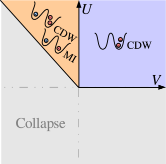
Figure 4: Phase diagram for $U,V$: different regions of stability and insulating phases for $t,j=0.$

Given that Eq. (26) and Eq. (27) are satisfied, the system is stable and we have two possibilities to attain the minimum energy: either at the boundaries, $n=0$ or $m=0,$ or right on the eigenvector of $A.$ Inspecting $\varepsilon_{B}$ and $\varepsilon_{+}$ we conclude that a positive value of $V$ will lead to the formation of charge density waves (CDW) of filled sites alternating with empty sites

$$V>0\,\Rightarrow\,n_{2k}=0~{}\mbox{or}~{}n_{2k+1}=0.$$ (28)

If $V\leq 0$ our energy functional will be convex and the minimum energy state will be a Mott insulator with $n=m,$ when $n+m$ is even, or a charge density wave with $n=m\pm 1,$ when $n+m$ is odd. The actual choice between these two insulating phases is obtained by computing the energy of both states

$$\epsilon(2n+1) = U(2n+1)^{2}/4+Vn(n+1)-(U+2\mu)(2n+1)/4$$ (29)

$$\epsilon(2n) = U(2n)^{2}/4+Vn^{2}-(U+2\mu)2n/4.$$ (30)

Having $\epsilon(2n+1)-\epsilon(2n)=0$ defines the value of $\mu$ at which the state with $2n$ particles every two sites, a Mott with $n$ particles, stops being the ground state and becomes more favorable to acquire an extra particle to form a CDW. The boundaries of these insulating phases for $t,j=0$ are given by

$$\mu(2n\to 2n+1)=(U+V)2n,$$ (31)

$$\mu(2n-1\to 2n)=(U+V)2n-U.$$ (32)

Thus summing up, for $\mu(2n-1\to 2n)\leq\mu\leq\mu(2n\to 2n+1)$ the optimal occupation is $n$ particles per site, forming a Mott, while for $\mu(2n\to 2n+1)\leq\mu\leq\mu(2n+1\to 2n+2)$ the occupation number is $2n+1$ particles spread over every two sites, having a CDW. The results of this section are summarized in Fig. 4.

4.2 Perturbation theory: insulator phase boundaries

The previous calculation can be improved using perturbation theory for $t,j\ll U,V$ around the insulating phases, obtaining the phase boundaries around the insulators as $t$ and $j$ are increased. This is done applying standard perturbation theory up to second order on both variables [25], using as unperturbed Hamiltonian the operator (4.1) and as perturbation the kinetic energy term

$$W=\sum_{i}\left\{-\left[t~{}c_{i}^{\dagger 2}c_{i+1}^{2}+j~{}(n_{i}-1)c^{\dagger}_{i}(c_{i-1}+c_{i+1})\right]+\mathrm{H.c.}\right\}.$$ (33)

We start calculating analytically the ground state energies of the first four insulating phases according to (4.1), considering the perturbation $W$ up to second order in $j,t.$ For the CDW with $n_{i}=1$ and $n_{i+1}=0$ this energy is obviously zero

$$E(L/2)=0.$$ (34)

For the MI with one particle per site we have virtual processes of the correlated hopping $j,$ as environment-assisted hopping starts being allowed in an uniformly filled lattice

$$E(L)=(U+2V)L/2-\frac{8j^{2}}{U-2V}L.$$ (35)

For the CDW with $n_{i}=2$ and $n_{i+1}=1,$ we find some doubly occupied sites and contributions from the pair hopping $t$

$$E(L+L/2)=(3U+4V)L/2-\left(\frac{6t^{2}}{U}+\frac{24j^{2}}{U-6V}+\frac{32j^{2}}{U+2V}\right)L.$$ (36)

Finally, for the MI with two particles per site, a calculation detailed in [26],

$$E(2L)=(3U+4V)L-\frac{24t^{2}+216j^{2}}{U-2V}L.$$ (37)

Here $L$ is the total number of sites and all results presented in this section are for the case $V<0.$

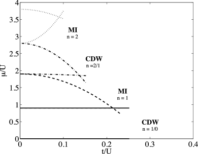
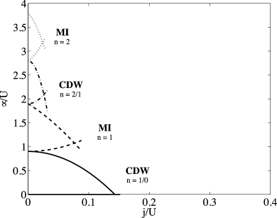
Figure 5: Phase diagrams for $\mu,$ $j,t\ll|U|$ and $V=-0.05.$ (left) Varying $t$ for $j=0.$ (right) Varying $j$ for $t=0.$ In both cases the lowest region is a CDW with alternating $0$ and $1$ particle occupation, followed upwards by a Mott of one particle per site, a CDW with $1$ and $2$ particles and the highest area a Mott of two particles.

At each value of $j,t,$ the boundary of an insulating phase with average density $\bar{n}$ is given by the degeneracy condition with a compressible state $E(\bar{n}L)=E(\bar{n}L\pm 1).$ Those points correspond to the chemical potential at which a hole, $\mu_{h}(\bar{n}L)=E(\bar{n}L)-E(\bar{n}L-1),$ or a particle, $\mu_{p}(\bar{n}L)=E(\bar{n}L+1)-E(\bar{n}L),$ can be introduced We show here the lower and upper limits of the first four insulating regions, corresponding to the CDW with $n_{i}=1,n_{i+1}=0$

$$\mu_{h}(L/2) = 0$$

$$\mu_{p}(L/2) = U+2V+j^{2}(\frac{2}{V}-\frac{4}{U})$$ (38)

the Mott with one particle per site

$$\mu_{h}(L) = U+2V+j^{2}\left(\frac{4}{U}-\frac{2}{V}-\frac{16}{U-2V}\right)$$ (39)

$$\mu_{p}(L) = E(L+1)-E(L)$$ (40)

$$= 2U+2V-8j-\frac{4j^{2}}{U}+\frac{2j^{2}}{V}+\frac{8(j^{2}-6jt-3t^{2})}{U-2V}$$

the CDW with $n_{i}=2,n_{i+1}=1$

$$\mu_{h}(L+L/2) = 2U+2V+\frac{48t^{2}V}{U^{2}-2UV}$$ (41)

$$+j^{2}\left(\frac{4}{U}-\frac{2}{V}+\frac{96}{U-6V}+\frac{24}{U-2V}+\frac{128}{U+2V}\right)$$

$$\mu_{p}(L+L/2) = E(L+L/2+1)-E(L+L/2)$$ (42)

$$= 3U+4V+j^{2}\left(-\frac{108}{U}+\frac{54}{V}+\frac{96}{U-6V}+\frac{64}{U+2V}\right)$$

$$+6t^{2}\left(\frac{4}{U}-\frac{8}{3U-2V}-\frac{4}{U-2V}-\frac{8}{U-6V}\right)$$

and the MI with two particles per site

$$\mu_{h}(2L) = 3U+4V+8j+\frac{108j^{2}}{U}+24t^{2}\left(\frac{2}{U-6V}+\frac{2}{3U-2V}\right)$$ (43)

$$-\frac{54j^{2}}{V}-\frac{24(35j^{2}-3\sqrt{2}jt+3t^{2})}{U-2V}$$

$$\mu_{p}(2L) = 4U+4V-6\sqrt{6}j-\frac{108j^{2}}{U}-\frac{48t^{2}}{U-6V}-\frac{48t^{2}}{3U-2V}$$ (44)

$$+\frac{54j^{2}}{V}+\frac{32(57j^{2}-12\sqrt{6}jt-7t^{2})}{3U-6V}$$

The corresponding boundaries are plotted in Fig. 5. For small hopping amplitude, they match the values that are found later on with the numerical methods. But even for larger values, this approximation anticipates that the lobes are significantly larger for pair hopping $t$ than for the correlated hopping $j.$

4.3 Phase model: analysis of the pair condensate

So far we have studied the many-body physics around the limit of strong interactions. However, the main goal of this work is to understand the effect of correlated hopping and the creation of a pair superfluid. In absence of a mean field theory, but still in the limit of dominant two-body hopping $U,V\ll t,$ we can use the number-phase representation, introduced in Ref. [27] for an ordinary BEC. Note, however, that the model in Ref. [27] cannot be directly applied here. Following that reference, one would assume a large number of particles per site, $n_{i}>1,$ and introduce the basis of phase states $|\vec{\phi}\rangle$

$$\langle\vec{n}|\vec{\phi}\rangle=(2\pi)^{-L/2}e^{i\vec{n}\cdot\vec{\phi}}.$$ (45)

Using these states, one would then develop approximate representations for the operators $a_{i}^{2},$ $a_{i}^{\dagger 2}$ and $n_{i},$ and diagonalize the resulting Hamiltonian in the limit of weak interactions. But after a few considerations one finds that the resulting phase model does not preserve an important symmetry of our system: if $j=0$ particles can only move in pairs and the parity of each site, $(-1)^{n_{i}},$ is a conserved quantity.

To describe correlated hopping we must use a basis of states with fixed parity $\nu$

$$\langle 2\vec{n}+\nu^{\prime}|\vec{\phi}\rangle_{\nu}=(2\pi)^{-L/2}e^{i\vec{n}\cdot\vec{\phi}}\delta_{\nu\nu^{\prime}},\quad\nu\in\{0,1\}$$ (46)

which is $\nu=0$ for the ground state we are interested in. As mentioned before, we now have to find expressions for the different operators, $a_{i}^{2},$ $a_{i}^{\dagger 2}$ and $n_{i}.$ We use the fact that our states will have a density close to the average value $\bar{n}$ and approximate the action of the operators over an arbitrary state as

$$n_{i}\left|{\vec{\phi}}\right\rangle = (-i2\partial_{\psi_{i}}-\bar{n})\left|{\vec{\phi}}\right\rangle,$$ (47)

$$a_{i}^{2}\left|{\vec{\phi}}\right\rangle = \sqrt{\bar{n}(\bar{n}-1)}e^{-i\phi_{i}}\left|{\vec{\phi}}\right\rangle,$$ (48)

$$a_{i}^{\dagger 2}\left|{\vec{\phi}}\right\rangle = \sqrt{(\bar{n}+1)(\bar{n}+2)}e^{i\phi_{i}}\left|{\vec{\phi}}\right\rangle.$$ (49)

Introducing the constant $\rho^{2}=\bar{n}(\bar{n}-1)(\bar{n}+1)(\bar{n}+2)$ our Hamiltonian becomes similar to the quantum rotor model [27]

$$H = \sum_{i=1}^{L}\left[2U\partial_{\phi_{i}}^{2}+(2U+4V)\partial_{\phi_{i}}\partial_{\phi_{i+1}}+2\rho^{2}t\cos\left(\phi_{i}-\phi_{i+1}\right)\right]$$ (50)

$$-(U+V)L\bar{n}^{2}.$$

For small $U$ and $V,$ the ground state of this model is concentrated around $\phi_{i}-\phi_{i+1}=0.$ Expanding the Hamiltonian up to second order in the phase fluctuations around this equilibrium point, we obtain a model of coupled harmonic oscillators. This new problem can be diagonalized using normal modes that are characterized by a quasi-momentum $k=2\pi n/L,$ $n\in[-(L-1)/2,(L-1)/2].$ The result is

$$H=\sum\hbar\omega_{k}\left(b_{k}^{\dagger}b_{k}+\frac{1}{2}\right)+E_{0}$$ (51)

with normal frequencies

$$\omega_{k}=4\rho\sqrt{2Ut}\left|\sin(k/2)\right|\sqrt{1+\left(1+\frac{2V}{U}\right)\cos\left(k\right)},$$ (52)

and a global energy shift $E_{0}=4(U+V)N^{2}-4L\bar{n}^{2}(U+V)-2\rho^{2}tL.$

It is evident from Eq. (52) that our derivation is only self consistent for negative values of $V.$ Otherwise, when $V>0$ some of the frequencies become imaginary, signaling the existence of an unbounded spectrum of modes with $|k|\geq\pi/4$ and that our ansatz becomes a bad approximation of the ground state. This strictly means that our choice $\phi_{i}=\phi_{i+1}$ only applies in the case of attractive nearest neighbor interactions, $-U\leq V\leq 0,$ as we know that this interaction cannot destabilize a translational invariant solution such as the uniform Mott insulator. However, it does not mean by itself that the whole system becomes unstable for $V>0$ — indeed, we will show numerically that it remains essentially in a similar phase for all values of $V,$ but in the case of $V>0$ the insulating phases are stable until values of the hopping slightly higher as in the $V<0$ case.

If we focus on the regime of validity, we will find that the spectrum is very similar to that of a condensate. At small momenta the dispersion relation becomes linear, $\omega_{k}\propto v_{g}k,$ with sound velocity $v_{g}=4\rho\sqrt{2Ut}/\hbar,$ while at larger energies the spectrum becomes quadratic, corresponding to “free” excitations with some mass. This a consequence of the similarity between our approximate model for the pairs (50) and the phase model for a one-dimensional condensate. However, we can go a step further and conclude that the similarity extends also to the wavefunctions themselves, so that the state of a pair superfluid can be obtained from that of an ordinary BEC by the transformation $n\to 2n.$ This is indeed consistent with what we obtained for the diagonalization of a two-particle state in the limit $j,U,V=0$ [See Eq. (15)].

5 Numerical methods

The previous sections draw a rather complete picture of the possible ground states in our model. In the limit of strong interactions we find both uniform insulators and a breakdown of translational invariance forming a CDW, while for dominant hopping we expect both single-particle superfluidity and a new phase, a pair superfluid. We now confirm these predictions using two different many-body variational methods.

5.1 Gutzwiller phase diagram

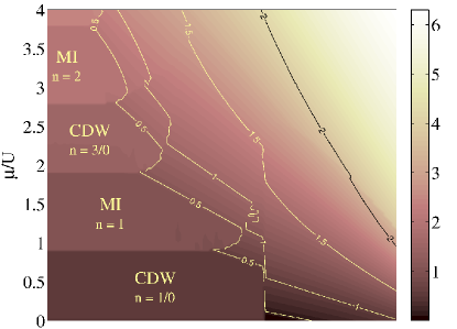
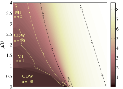
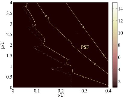
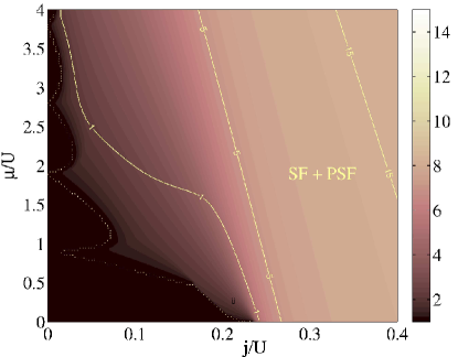
Figure 6: Phase diagram with a Gutzwiller ansatz for $U=1,V=-0.5.$ We focus on (left) $j=0$ and (right) $t=0,$ separately. Upper plots show average site occupation $\langle n\rangle$ (grayscale), and number variance $\Delta n$ (contour). Lower plots show single-particle coherence $\langle a\rangle$ (grayscale) together with $\Delta a^{2}$ (contour).

The first method that we use is a variational estimate of ground state properties based on a product state [28]

$$|\psi_{\mathrm{GW}}\rangle=\prod_{i}\sum_{n_{i}}f_{n}^{(i)}\frac{1}{\sqrt{n_{i}!}}c_{i}^{\dagger n_{i}}\left|{0}\right\rangle.$$ (53)

Minimizing the expectation value of the free energy $F=H-\mu N$ with respect to the variables $f_{n},$ under the constrain of fixed norm $\sum_{n}|f_{n}|^{2}=1,$ we will obtain the phase diagram in the phase space of interactions and chemical potential $(U,V,j,t,\mu).$

In our study we have made several simplifications. First of all, we assumed period-two translational invariance in the wavefunction, using only two different sets of variational parameters, $f_{n}^{(2i+1)}=f_{n}^{1}$ and $f_{n}^{(2i)}=f_{n}^{0}.$ In our experience, this is enough to reproduce effects such as the CDW. Next, since $U\geq 0$ is required for the stability of the system, we have taken $U=1$ as unit of energy. The limit $U=0$ is approximated by the limits $j,t\gg 1$ in our plots. Finally, in order to determine the roles of $j$ and $t,$ we have studied the cases $j=0$ and $t=0$ separately.

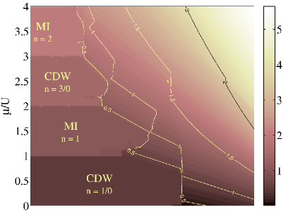
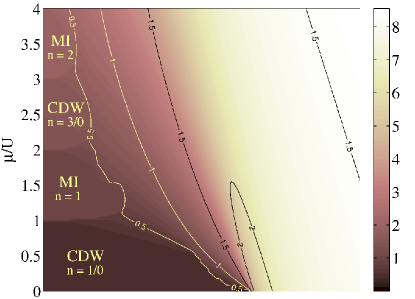
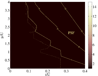
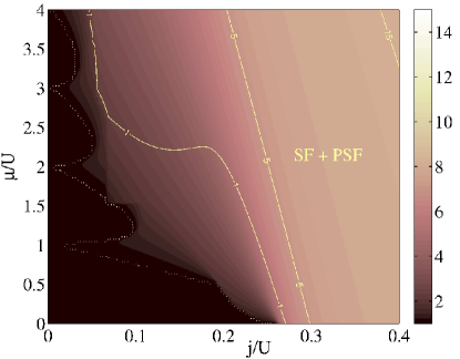
Figure 7: Phase diagram with a GW ansatz for $U=1,V=0.5.$ We focus on (left) $j=0$ and (right) $t=0,$ separately. Upper plots show average site occupation $\langle n\rangle$ (grayscale) and number variance $\Delta n$ (contour). Lower plots show single-particle coherence $\langle a\rangle$ (grayscale) together with $\Delta a^{2}$ (contour).

The results are shown in Fig. 6 and Fig. 7 for $V<0$ and $V>0,$ respectively.

The first interesting feature is that, as predicted by perturbation theory, we have large lobes both with integer $1,2,\ldots$ and with fractional $1/0,2/1,\ldots$ occupation numbers, forming uniform Mott insulators and CDW, respectively. The insulators are characterized by having a well defined number of particles per site, and thus no number fluctuations $\Delta n^{2}=\langle n^{2}\rangle-\langle n\rangle^{2}=0.$ While the size of the lobes does not depend dramatically on the sign of $V,$ these are significantly larger for the pair hopping $t$ than for the correlated hopping $j,$ as already seen with perturbation theory.

The boundary of the insulating areas marks a second order phase transition to a superfluid regime, where we find number fluctuations $\Delta n\neq 0.$ In order to characterize these gapless phases we have computed the order parameter of a single-particle condensate $\langle a\rangle,$ and two quantities that we use to detect pairing. The first one is a two-particle correlation that generalizes the order parameter of a BEC to the case of a pair-BEC $\langle a^{2}\rangle.$ The second quantity $\Delta a^{2}=|\langle a^{2}\rangle-\langle a\rangle^{2}|$ is used to correct the previous value eliminating the contribution that may come from a single-particle condensate coexisting with the pair-BEC.

When $j=0$ we always find that $\langle a\rangle=0,$ even outside the insulating lobes. This marks the absence of a single-particle BEC, which is expected since we do not have single-particle hopping. On the other hand, we now find long range coherence of the pairs and thus $\langle a^{2}\rangle\neq 0$ all over the non-insulating area, which we identify with the pair-superfluid regime.

The situation is slightly different for $t=0.$ The single-particle order parameter $\langle a\rangle$ no longer vanishes in the superfluid area, denoting the existence of single-particle coherence, but at the same time we find that the two-particle correlations exceed the contribution from the single-particle superfluid as $\Delta a^{2}\neq 0,$ which we attribute to a coexistence of both a single-particle and a pair-superfluid, or a state with both features.

This picture does not change substantially when $V$ is positive or negative. The only differences are in the insulating regions, where the CDW is either due to the incommensurability of the particle number $(V<0)$ or really gives rise to the separation of particles alternating holes and filled sites $(V>0).$ However, in the superfluid regime we find no significant changes and in particular we see no breaking of the translational invariance or modulation of the coherent phase.

5.2 Matrix Product States: long range pair correlations

The previous numerical simulations are very simple and cannot fully capture the single particle and two-particle correlators. To complete and verify the full picture we have searched the ground states of the full Hamiltonian using the so called iTEBD algorithm, which uses an infinite Matrix Product State ansatz together with imaginary time evolution [29].

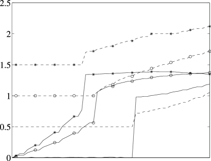
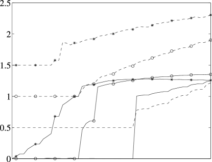
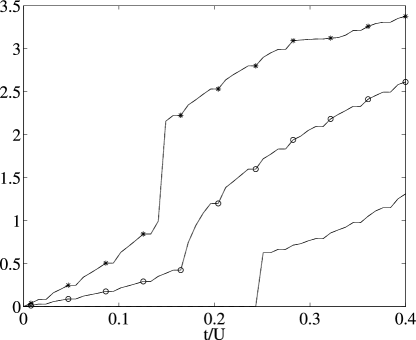
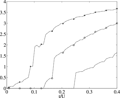
Figure 8: Numerical simulations with the iTEBD algorithm. On the left we plot the results for $j=0,U=1,V=-0.05$ and on the right for $V=0.05,$ as a function of two-particle tunneling $t.$ The upper row shows the density (dashed) and particle number fluctuations (solid), while the lower row shows $(\Delta a)^{2}$ (solid) and two-particle coherence (dashed), which overlap indicating $\langle a\rangle=0.$ For each set of operators we show three lines, for $\mu/U=0.5,~{}1.5$ and $2.5$ corresponding to plain line, circle and star, respectively.

Roughly, this ansatz is based on an infinite contraction of tensors that approximates the wavefunction of a translational invariant system in the limit of infinite size. Adapting the ansatz to our problem we write it as

$$\left|\psi\right\rangle\sim\prod_{k\in\mathbb{Z}}\Gamma^{o}_{\alpha_{2k+1}\alpha_{2k+2}}(n_{2k+1})\lambda^{o}_{\alpha_{2k+2}}\Gamma^{e}(n_{2k+2})_{\alpha_{2k+2}\alpha_{2k+3}}\lambda^{e}_{\alpha_{2k+3}}\times$$

$$\quad\quad\quad\quad\times\frac{1}{\sqrt{n_{2k+1}!n_{2k+2}!}}a^{\dagger n_{2k+1}}_{2k+1}a^{\dagger n_{2k+2}}_{2k+2}\left|\mathrm{vac}\right\rangle.$$ (54)

Here the $\Gamma^{o}$ and $\Gamma^{e}$ are matrices that depend on the state of the odd and even sites they represent, a dependence which is signaled by the $n_{2k+1}$ and $n_{2k+2}$ in the previous equation. These matrices are contracted with one-dimensional vectors of positive weights $\lambda^{e,o}_{\alpha}\geq 0,$ which are related to the coefficients of the Schmidt decomposition. This variational ansatz is known to work well for states with fast decaying correlations, but it also gives a good qualitative description of the critical phases.

In order to optimize the iTEBD wavefunction we performed an approximate imaginary time evolution using a Trotter decomposition and local updates of the associated tensors, as described in Ref. [30]. Using the canonical forms for these tensors it is also straightforward to compute expectation values for different operators acting either on neighboring or separated sites.

In Fig. 8 we plot the most relevant results for three cuts across the phase diagram, $\mu=0.5,~{}1.5$ and $2.5,$ so that each line crosses both an insulating plateau and the superfluid region. We have used small tensor sizes from $D=16$ up to $64,$ a value limited by the need of using large cutoffs for the site populations ($n_{max}=8$). As shown in the figures, when $j=0$ the single-particle correlator is zero for distinct sites, and we are left only with two-particle correlations. In the MI case the pair correlations between neighboring sites decrease very quickly, while in the superfluid regime we see a critical behavior

$$C^{2}_{\Delta}\propto\frac{1}{\Delta^{\alpha}},$$ (55)

with an exponent that varies between $\alpha=0.5$ and $\alpha=0.6,$ depending on the simulation parameters.

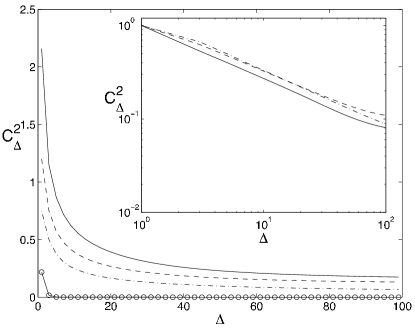
Figure 9: Correlator $C^{2}_{\Delta}=\langle{a^{\dagger 2}_{i+\Delta}a^{2}_{i}}\rangle$ vs. site separation, for $(t,\mu)$ $=$ $(0.1,1.5),$ $(0.3,0.5),$ $(0.2,1.5),$ $(0.1,2.5)$, from top to bottom. The line with $t=0.1,\mu=1.5$ (solid, circles) corresponds to a MI state and correlations decay to zero on the third site. The remaining lines have been rescaled and plotted in log-log scale in the inset, which shows that the two-particle correlator decays approximately as $\Delta^{-\alpha}$ with a power $\alpha\sim 0.5-0.6.$

6 Detection

There are many ways of differentiating the phases we have found, each one having its own degree of difficulty. The simplest and best established detection methods are related to the insulating regimes. These phases, which involve both MI and CDW, are characterized by having a well defined number of particles at each lattice site, the lack of coherence and an energy gap that separates the insulator from other excitations.

The energy gap in these insulators may be probed either by static or spectroscopic means as it has been done in experiments [7, 31], determining that indeed the system is insulating. Second, the lack of coherence will translate into featureless time-of-flight images, having no interference fringes [7] at all. Even though there will be no fringes, the measured density will be affected by quantum noise. The analysis of the noise correlation will show peaks at certain momenta [32, 33] that depend on the periodicity of the state, so that the number of peaks in the CDW phase will be twice those of the MI. In case of having access to the lattice sites, as in the experiments with electron microscopy [34], or in future experiments with large aperture microscopic objectives that can collect the fluorescence of individual lattice sites [35, 36], the discrimination between the MI and the CDW should be even easier, since in one case we have a uniform density and in the other a periodic distribution of atoms.

When the system enters a superfluid phase, it becomes a perfect “conductor” with a gapless excitation spectrum. The lack of an energy gap, should be evident in the spectroscopic experiments suggested before. However, we are not only interested in the superfluid nature, but rather in the fact that this quantum phase is strongly paired. More precisely, we have found that for $j=0$ the single-particle coherence is small or zero, and that the two-particle correlator decays slowly

$$C^{1}_{\Delta} = \langle a^{\dagger}_{i}a_{i+\Delta}\rangle\sim\bar{n}\delta_{\Delta 0}$$ (56)

$$C^{2}_{\Delta} = \langle a^{\dagger 2}_{i}a^{2}_{i+\Delta}\rangle\sim 1/\Delta^{\alpha}.$$ (57)

The first equation implies that the time of flight images will reveal no interference fringes and will exhibit noise correlations which will be similar to the MI. In order to probe $C^{2}_{\Delta}$ and confirm the pairing of the particles, we suggest to use Raman photo-association to build molecules out of pairs of atoms [37, 38]. For an efficient conversion, it would be best to perform an adiabatic passage from the free atoms to the bound regime. As described in [39], we expect a mapping that goes from $\left|2n\right\rangle\rightarrow\left|n\right\rangle,$ where $2n$ is the number of bosons and $n$ the number of molecules. More precisely, we expect the $a^{\dagger 2}$ operator to be mapped into $m^{\dagger},$ so that the pair coherence of the original atoms translates into the equivalent of $C^{1}_{\Delta}$ for the molecules. This order should reveal as an interference pattern in time-of-flight images of the molecules.

Finally, in cases with $j\neq 0,$ we have found the coexistence of single-particle and two-particle coherences. This translates also into the coexistence of interference fringes with nonzero pair correlators.

7 Conclusions

Summing up, we have suggested a family of experiments with cold atoms that would produce correlated hopping of bosons. The mechanism for the correlated hopping is an asymmetry in the contact interaction between atoms. This asymmetry is exploited by trapping the atoms in dressed states, a configuration that gives rise to transport induced by collisions.

The main result of this paper is that there is a huge variety of interaction asymmetries that will give rise to long range pair correlations via interaction–induced transport. Formally, in the resulting effective models we recognize two dynamical behaviors. If we have a nonzero asymmetry in the interspecies interactions,

$$t\propto 2g_{\uparrow\downarrow}-g_{\uparrow\uparrow}-g_{\downarrow\downarrow}\neq 0,$$

the Hamiltonian will exhibit pair hopping, while an asymmetry in the intra-species scattering lengths

$$j\propto g_{\uparrow\uparrow}-g_{\downarrow\downarrow}\neq 0,$$

gives rise to correlated hopping. However, we have given enough evidence that both Hamiltonian terms give rise to a novel quantum phase which we call pair superfluid. This phase is characterized by a gapless spectrum with a finite sound speed, zero single-particle correlations and long range pair coherence. All quantum phases are connected by second order quantum phase transitions. These phases can be produced and identified using variations of current experiments [40, 41, 33]. The nonperturbative nature of the effect should help in that respect.

Our ideas are not restricted to one dimension. It is possible to engineer also a two–body hopping using two–dimensional lattice potentials. Again, the basic ingredients would be atoms with an asymmetric interaction and an optical lattice that traps two states, $\left|{+}\right\rangle$ and $\left|{-}\right\rangle$ with a relative displacement. Both in the one– and two–dimensional cases it is a valid question to ask whether the coupling between different trapped states, $\left|{\pm}\right\rangle,$ can excite also transitions to higher bands, processes that have not been considered in the paper. Our answer here is no. There are only two sources of coupling to higher energy bands. One is the interaction, but we are already assuming that the interaction energies are much smaller than the band separation. Following the notation from Ref. [8], we have the constraint that the interaction energy should be smaller than the energy separation to the first excited state in a well of the periodic potential, $\bar{n}^{2}U\ll\hbar\bar{\nu}\bar{n}$ the same requisite as for ordinary Bose–Hubbard models [7]. The other source of coupling to higher bands would be single–particle hopping. However, unlike [8], here we are assuming that these terms are strongly suppressed compared with the interaction. In other words, realizing the models that we suggest in this paper, for realistic densities, $\bar{n}=2,$ and simple potentials, imposes no further constraint in current experiments.

Finally, let us remark that transport–inducing collisons may be implemented using other kinds of spin-dependent interactions. For instance, correlated hopping appears naturally in state-dependent lattices loaded with spinor atoms, because their interactions can change the hyperfine state of the atoms while preserving total angular momentum [42].

We would like to thank Miguel Angel Martín-Delgado for useful discussions. M.E. acknowledges support from the CONQUEST project. J.J.G.R acknowledges financial support from the Ramon y Cajal Program of the Spanish M.E.C., from U.S. NSF Grant No. PHY05-51164 and from the spanish projects FIS2006-04885 and CAM-UCM/910758.

Appendix A Derivation of the model in superlattices

As discussed before, the main idea behind atomic correlated hopping is to trap atoms whose interaction allows them to change their state. In this section we provide one possible implementation of this idea using state dependent superlattices that trap dressed states.

A.1 Dressed states trapping

Our starting point is the setup in Fig. 2a, which is itself taken from Ref. [43]. It consists on an optical lattice trapping atoms in states $\left|{\uparrow}\right\rangle$ and $\left|{\downarrow}\right\rangle,$ together with a Raman coupling between these states. Mathematically, this configuration is described by the single-particle Hamiltonian

$$H_{\mathrm{trap}} = V_{0}~{}\sin(kx)^{2}\left(\left|{\uparrow}\right\rangle\left\langle{\uparrow}\right|+\left|{\downarrow}\right\rangle\left\langle{\downarrow}\right|\right)$$ (58)

$$+\Omega~{}\sin(kx)\left(\left|{\uparrow}\right\rangle\left\langle{\downarrow}\right|+\left|{\downarrow}\right\rangle\left\langle{\uparrow}\right|\right).$$

By moving to the basis of dressed states $\left|{\pm}\right\rangle=\frac{1}{\sqrt{2}}\left(\left|{\uparrow}\right\rangle\pm\left|{\downarrow}\right\rangle\right),$ we find that the trapping is effectively equivalent to two superlattices with a relative displacement as in Fig. 2b

$$H_{\mathrm{trap}} = \left(V_{0}\sin(kx)^{2}+\Omega\sin(kx)\right)\left|{+}\right\rangle\left\langle{+}\right|$$ (59)

$$+\left(V_{0}\sin(kx)^{2}-\Omega\sin(kx)\right)\left|{-}\right\rangle\left\langle{-}\right|.$$

Under appropriate circumstances, discussed in [43], we will find that each superlattice site has a unique ground state, energetically well differentiated from the next excited state, and which consists of a symmetric wavefunction spanning both lattice wells. If this is the case and if all energy scales, such as the interaction and the hopping, are small compared to the separation between Bloch bands, we can expand the bosonic field operators describing the atoms in terms of these localized wavefunctions

$$\psi_{+}(x)=\sum_{i}c_{2i}~{}W(x-2il),$$ (60)

$$\psi_{-}(x)=\sum_{i}c_{2i+1}~{}W(x-(2i+1)l),$$

where $2l=2\pi/k$ is the superlattice period, $c_{j}$ are bosonic operators that, for $j$ even (odd), annihilate an atom in state $\left|{+}\right\rangle$ ($\left|{-}\right\rangle$) in the $j$-th superlattice cell

$$c_{2i}=\frac{1}{\sqrt{2}}(a_{2i,+}+a_{2i+1,+}),$$ (61)

$$c_{2i+1}=\frac{1}{\sqrt{2}}(a_{2i+1,-}+a_{2i+2,-}),$$

and the localized wavefunctions $W(x)$ are a superposition of the Wannier functions $w(x^{\prime})$ of the underlying lattice

$$W(x-2il)=\frac{1}{\sqrt{2}}\left[w(x-2il)+w(x-(2i+1)l)\right].$$ (62)

A.2 State-changing collisions

We will now express the interaction (4) in the basis of dressed states. We proceed using the change of variables in Eq. 6 to find the expression of the densities

$$\rho_{\uparrow}(x) = \frac{1}{2}(\rho_{+}+\rho_{-}+\psi_{+}^{\dagger}\psi_{-}+\psi_{-}^{\dagger}\psi_{+}),$$ (63)

$$\rho_{\downarrow}(x) = \frac{1}{2}(\rho_{+}+\rho_{-}-\psi_{+}^{\dagger}\psi_{-}-\psi_{-}^{\dagger}\psi_{+}).$$ (64)

The first obvious conclusion is that the total density is independent of the basis on which it is written,

$$\rho(x)=\rho_{\uparrow}(x)+\rho_{\downarrow}(x)=\rho_{+}(x)+\rho_{-}(x).$$ (65)

Hence, the term of $g_{0}$ is insensitive to the state of the atoms. On the other hand, the asymmetric terms are not so simple. The $g_{1}$ interaction, which is proportional to the product of densities

$$:\rho_{\uparrow}\rho_{\downarrow}: = \frac{1}{4}:(\rho_{+}+\rho_{-})^{2}:-\frac{1}{4}:(\psi_{+}^{\dagger}\psi_{-}+\psi_{-}^{\dagger}\psi_{+})^{2}:$$ (66)

$$= \frac{1}{4}:(\rho_{+}+\rho_{-})^{2}:-\frac{1}{2}\rho_{+}\rho_{-}-\frac{1}{4}(\psi_{+}^{\dagger 2}\psi_{-}^{2}+H.c)$$

$$= \frac{1}{4}:\rho_{+}^{2}+\rho_{-}^{2}:-\frac{1}{4}(\psi_{+}^{\dagger 2}\psi_{-}^{2}+H.c),$$

gives rise to a scattering that changes the state of interacting atoms from $\left|{-}\right\rangle$ to $\left|{+}\right\rangle$ and viceversa, as in Fig. 1a. The term of $g_{2}$ has a lightly different effect,

$$:\rho_{\uparrow}(x)^{2}-\rho_{\downarrow}(x)^{2}:=:\rho(x)\left[\psi^{\dagger}_{+}(x)\psi_{-}(x)+\psi^{\dagger}_{-}(x)\psi_{+}(x)\right]:$$ (67)

it gives rise to processes where one atom changes its state influenced by the surrounding environment. In the following subsections we will see what happens to the interaction terms (65), (66) and (67), when the atoms are confined in a lattice.

A.3 Final model

In this section we will put the previous results of this appendix together. We will take the tight-binding expansion of the field operators (60) and use it together with Eqs. (65), (66) and (67) to expand the interaction Hamiltonian (4). For convenience, we will rename the bosonic operators as

$$c_{2k}=a_{k+}~{}~{}\mathrm{and}~{}~{}c_{2k+1}=a_{k-}$$ (68)

according to the position at which their Wannier functions are centered (see Fig. 2c). Along the derivation, one obtains many integrals of ground state wavefunctions

$$C_{k,m}=\int|W(x-kl)|^{2}|W(x-ml)|^{2}dx.$$ (69)

We will only keep those integrals with a separation smaller than a superlattice period. Taking Eq. (62), the expression for the superlattice localized states, one obtains

$$C_{k,k} = \int|W(x)|^{4}dx\simeq\frac{1}{2}\int|w(x)|^{4}dx,$$ (70)

$$C_{k,k\pm 1} = \int|W(x)|^{2}|W(x-l)|^{2}dx\simeq\frac{1}{4}\int|w(x)|^{4}dx,$$ (71)

where $w(x)$ are the Wannier wavefunctions of the underlying sublattice. Using these tools, the symmetric interaction term becomes

$$~{}~{}~{}~{}~{}\frac{g_{0}}{2}\int dx:(\rho_{\uparrow}(x)+\rho_{\downarrow}(x))^{2}:=$$

$$=\frac{g_{0}}{2}\sum_{k}^{N/2}:n_{2k}^{2}C_{2k,2k}+n_{2k+1}^{2}C_{2k+1,2k+1}+2n_{2k}n_{2k+1}C_{2k,2k+1}:$$

$$=\frac{g_{0}}{4}\int dx~{}|w(x)|^{4}~{}\sum_{k}^{N}:n_{k}^{2}+n_{k}n_{k+1}:$$ (72)

For the asymmetric parts, we first use Eq. (66) obtaining

$$~{}~{}~{}~{}~{}g_{1}\int dx:\rho_{\uparrow}(x)\rho_{\downarrow}(x):=$$

$$\frac{g_{1}}{8}\int dx~{}|w(x)|^{4}~{}\sum_{k}^{N}\left[:n_{k}^{2}:-~{}\frac{1}{2}\left(c_{k+1}^{\dagger 2}c_{k}^{2}+c_{k}^{\dagger 2}c_{k+1}^{2}\right)\right]$$ (73)

and then finally the more complicated Eq. (67)

$$~{}~{}~{}~{}~{}\frac{g_{2}}{2}\int dx:\rho_{\uparrow}(x)^{2}-\rho_{\downarrow}(x)^{2}:=$$

$$\frac{g_{2}}{8}\int dx~{}|w(x)|^{4}\sum_{k}^{N}:n_{k}(c_{k}^{\dagger}c_{k-1}+c_{k-1}^{\dagger}c_{k}+c_{k}^{\dagger}c_{k+1}+c_{k+1}^{\dagger}c_{k}):$$ (74)

Introducing constants that parameterize the on-site interactions and the strength of the underlying lattice (7), our final Hamiltonian looks as follows

$$H = \frac{2U_{0}+U_{1}}{8}\sum_{k}:n_{k}^{2}:-\frac{U_{0}}{8}\sum_{k}:n_{k}n_{k+1}:-\frac{U_{1}}{16}\sum_{k}(c^{\dagger 2}_{k+1}c^{2}_{k}+\mathrm{H.c.})$$ (75)

$$-\frac{U_{2}}{8}\sum_{k}\left[(n_{k}-1)c^{\dagger}_{k}(c_{k-1}+c_{k+1})+\mathrm{H.c.}\right].$$

Completing terms and replacing the sum over $k$ with a sum over nearest neighbors, we arrive at the desired model (1) with the parametrization given already in Eq. (8).

References

References

- [1] M. H. Anderson, J. R. Ensher, M. R. Matthews, C. E. Wieman, and E. A. Cornell. Observation of Bose-Einstein Condensation in a Dilute Atomic Vapor. Science, 269:198, July 1995.
- [2] K. B. Davis, M.-O. Mewes, M. R. Andrews, N. J. van Druten, D. S. Durfee, D. M. Kurn, and W. Ketterle. Bose-Einstein condensation in a gas of sodium atoms. Phys. Rev. Lett., 75:3969, November 1995.
- [3] C. C. Bradley, C. A. Sackett, J. J. Tollett, and R. G. Hulet. Evidence of Bose-Einstein Condensation in an Atomic Gas with Attractive Interactions. Phys. Rev. Lett., 75:1687, August 1995.
- [4] C. A. Regal, M. Greiner, and D. S. Jin. Observation of Resonance Condensation of Fermionic Atom Pairs. Phys. Rev. Lett., 92(4):040403, January 2004.
- [5] M. W. Zwierlein, C. A. Stan, C. H. Schunck, S. M. Raupach, A. J. Kerman, and W. Ketterle. Condensation of Pairs of Fermionic Atoms near a Feshbach Resonance. Phys. Rev. Lett., 92(12):120403, March 2004.
- [6] T. Bourdel, L. Khaykovich, J. Cubizolles, J. Zhang, F. Chevy, M. Teichmann, L. Tarruell, S. J. Kokkelmans, and C. Salomon. Experimental Study of the BEC-BCS Crossover Region in Lithium 6. Phys. Rev. Lett., 93(5):050401, July 2004.
- [7] M. Greiner, O. Mandel, T. Esslinger, T. W. Hänsch, and I. Bloch. Quantum phase transition from a superfluid to a Mott insulator in a gas of ultracold atoms. Nature, 415:39, January 2002.
- [8] D. Jaksch, C. Bruder, J. I. Cirac, C. W. Gardiner, and P. Zoller. Cold Bosonic Atoms in Optical Lattices. Phys. Rev. Lett., 81:3108, October 1998.
- [9] L.-M. Duan, E. Demler, and M. D. Lukin. Controlling Spin Exchange Interactions of Ultracold Atoms in Optical Lattices. Phys. Rev. Lett., 91(9):090402, August 2003.
- [10] J. J. García-Ripoll and J. I. Cirac. Spin dynamics for bosons in an optical lattice. New J. Phys., 5:76, June 2003.
- [11] B. Paredes, P. Fedichev, J. I. Cirac, and P. Zoller. 1/2-Anyons in Small Atomic Bose-Einstein Condensates. Phys. Rev. Lett., 87(1):010402, July 2001.
- [12] D. Jaksch and P. Zoller. Creation of effective magnetic fields in optical lattices: the Hofstadter butterfly for cold neutral atoms. New J. Phys., 5:56, May 2003.
- [13] K. Osterloh, M. Baig, L. Santos, P. Zoller, and M. Lewenstein. Cold Atoms in Non-Abelian Gauge Potentials: From the Hofstadter ”Moth” to Lattice Gauge Theory. Phys. Rev. Lett., 95(1):010403, June 2005.
- [14] M. Eckholt and J. J. García-Ripoll. Pair condensation of bosonic atoms induced by optical lattices. Physical Review A (Atomic, Molecular, and Optical Physics), 77(6):063603, 2008.
- [15] M. R. Matthews, B. P. Anderson, P. C. Haljan, D. S. Hall, C. E. Wieman, and E. A. Cornell. Vortices in a bose-einstein condensate. Phys. Rev. Lett., 83(13):2498, Sep 1999.
- [16] M. E. Foglio and L. M. Falicov. New approach to the theory of intermediate valence. i. general formulation. Phys. Rev. B, 20(11):4554, Dec 1979.
- [17] I. N. Karnaukhov. Model of fermions with correlated hopping (integrable cases). Phys. Rev. Lett., 73:1130, August 1994.
- [18] I. N. Karnaukhov. Karnaukhov replies:. Phys. Rev. Lett., 74(26):5285, Jun 1995.
- [19] L. Arrachea, A. A. Aligia, E. Gagliano, K. Hallberg, and C. Balseiro. Superconducting correlations in hubbard chains with correlated hopping. Phys. Rev. B, 50(21):16044, Dec 1994.
- [20] L. Arrachea and A. A. Aligia. Exact solution of a Hubbard chain with bond-charge interaction. Phys. Rev. Lett., 73:2240, October 1994.
- [21] J. de Boer, V. E. Korepin, and A. Schadschneider. pairing as a mechanism of superconductivity in models of strongly correlated electrons. Phys. Rev. Lett., 74(5):789, Jan 1995.
- [22] J. Vidal and B. Douçot. Strongly correlated hopping and many-body bound states. Phys. Rev. B, 65(4):045102, Dec 2001.
- [23] J. E. Hirsch. Bond-charge repulsion and hole superconductivity. Physica C, 158:326, May 1989.
- [24] F. Marsiglio and J. E. Hirsch. Hole superconductivity and the high- oxides. Phys. Rev. B, 41(10):6435, Apr 1990.
- [25] J. K. Freericks and H. Monien. Strong-coupling expansions for the pure and disordered bose-hubbard model. Physical Review B, 53(5):2691, Feb 1996.
- [26] M. Eckholt. Strong correlation effects with atoms in optical lattices. PhD thesis.
- [27] J. J. García-Ripoll, J. I. Cirac, P. Zoller, C. Kollath, U. Schollwöck, and J. von Delft. Variational ansatz for the superfluid Mott-insulator transition in optical lattices. Optics Express, 12:42, January 2004.
- [28] W. Krauth, M. Caffarel, and J.-P. Bouchaud. Gutzwiller wave function for a model of strongly interacting bosons. Phys. Rev. B, 45:3137, February 1992.
- [29] G. Vidal. Classical simulation of infinite-size quantum lattice systems in one spatial dimension. Physical Review Letters, 98(7):070201, 2007.
- [30] R. Orús and G. Vidal. Infinite time-evolving block decimation algorithm beyond unitary evolution. Physical Review B (Condensed Matter and Materials Physics), 78(15):155117, 2008.
- [31] T. Stöferle, H. Moritz, C. Schori, M. Köhl, and T. Esslinger. Transition from a Strongly Interacting 1D Superfluid to a Mott Insulator. Phys. Rev. Lett., 92(13):130403, March 2004.
- [32] E. Altman, E. Demler, and M. D. Lukin. Probing many-body states of ultracold atoms via noise correlations. Phys. Rev. A, 70(1):013603, July 2004.
- [33] S. Fölling, F. Gerbier, A. Widera, O. Mandel, T. Gericke, and I. Bloch. Spatial quantum noise interferometry in expanding ultracold atom clouds. Nature, 434:481, March 2005.
- [34] T. Gericke, P. Wurtz, D. Reitz, T. Langen, and H. Ott. High-resolution scanning electron microscopy of an ultracold quantum gas. Nature Physics, October 2008.
- [35] K. D. Nelson, X. Li, and D. S. Weiss. Imaging single atoms in a three-dimensional array. Nat Phys, 3:556, 2007.
- [36] M. Karski, L. Förster, J. M. Choi, W. Alt, A. Widera, and D. Meschede. Nearest-neighbor detection of atoms in a 1d optical lattice by fluorescence imaging. Physical Review Letters, 102(5):053001, 2009.
- [37] P. S. Julienne, K. Burnett, Y. B. Band, and W. C. Stwalley. Stimulated raman molecule production in bose-einstein condensates. Phys. Rev. A, 58(2):R797, Aug 1998.
- [38] R. Wynar, R. S. Freeland, D. J. Han, C. Ryu, and D. J. Heinzen. Molecules in a Bose-Einstein Condensate. Science, 287(5455):1016, 2000.
- [39] J. J. García-Ripoll. Time evolution of matrix product states. New Journal of Physics, 8(12):305, 2006.
- [40] M. Anderlini, J. Sebby-Strabley, J. Kruse, J. V. Porto, and W. D. Phillips. Controlled atom dynamics in a double-well optical lattice. J. Phys. B: At. Mol. Opt. Phys., 39:199, May 2006.
- [41] J. Sebby-Strabley, M. Anderlini, P. S. Jessen, and J. V. Porto. Lattice of double wells for manipulating pairs of cold atoms. Phys. Rev. A, 73(3):033605–+, March 2006.
- [42] A. Widera, F. Gerbier, S. Folling, T. Gericke, O. Mandel, and I. Bloch. Precision measurement of spin-dependent interaction strengths for spin-1 and spin-2 87rb atoms. New J. Phys., 8(8):152, 2006.
- [43] J. J. García-Ripoll and J. K. Pachos. Fragmentation and destruction of the superfluid due to frustration of cold atoms in optical lattices. New J. Phys., 9(5):139, 2007.