Probing Reionization with Quasar Spectra: the Impact of the Intrinsic Lyman- Emission Line Shape Uncertainty

Abstract

Arguably the best hope of understanding the tail end of the reionization of the intergalactic medium (IGM) at redshift $z>6$ is through the detection and characterization of the Gunn-Peterson (GP) damping wing absorption of the IGM in bright quasar spectra. However, the use of quasar spectra to measure the IGM damping wing requires a model of the quasar’s intrinsic Lyman- emission line. Here we quantify the uncertainties in the intrinsic line shapes, and how those uncertainties affect the determination of the IGM neutral fraction. We have assembled a catalog of high-resolution HST spectra of the emission lines of unobscured low-redshift quasars, and have characterized the variance in the shapes of their lines. We then add simulated absorption from the high-redshift IGM to these quasar spectra in order to determine the corresponding uncertainties in reionization constraints using current and future samples of $z>6$ quasar spectra. We find that, if the redshift of the Lyman- emission line is presumed to coincide with the systemic redshift determined from metal lines, the inferred IGM neutral fraction is systematically biased to low values due to a systematic blueshift of the Lyman- line relative to the metal lines. If a similar blueshift persists in quasars at $z>6$, this bias strengthens previous claims of a significant neutral hydrogen fraction at $z\approx 6$. The bias can be reduced by including a Lyman- blueshift in the modeling procedure, or by excising wavelengths near the Lyman- line center from the modeling. Intrinsic Lyman- line shape variations still induce significant scatter in the inferred $x_{\mathrm{IGM}}$ values. Nevertheless, this scatter still allows a robust distinction between a highly ionized ($x_{\mathrm{IGM}}\sim 10^{-3}$) and a neutral ($x_{\mathrm{IGM}}=1$) IGM with even a few bright quasars. We conclude that if the variations of the intrinsic Lyman- emission line shapes in high-$z$ quasars are similar to those at low-$z$, this variation will not limit the usefulness of quasar spectra in probing reionization.

1 Introduction

One of the most important frontiers of observational astronomy is the study of the reionization of the universe. The details of reionization — when it started, how long it took, and what types of objects contributed ionizing photons — hold clues to the birth and early history of the various structures we see in the universe today. Because of their high luminosities and relatively flat spectra, quasars are excellent probes of reionization. Many efforts have been made to constrain the ionization state of the intergalactic medium (IGM), and thus the timing of the tail-end of reionization, using spectra of $z>6$ quasars discovered by the Sloan Digital Sky Survey (Fan, Carilli & Keating, 2006, and references therein). Beginning at lower redshift, the forest of Lyman- absorption lines in a quasar spectrum traces the fluctuating neutral hydrogen density along the line of sight. At $z\sim 6$, the Lyman- forest lines blend together and saturate, forming the dark Gunn-Peterson trough (Gunn & Peterson, 1965), indicating a neutral fraction of $\ga 10^{-3}$(Fan et al., 2006). This saturation at such a small neutral fraction limits the utility of Lyman-series absorption spectra as direct probes of the reionization epoch, though the scattered transmission windows in this otherwise dark trough do contain some information about the IGM ionization state (Fan et al., 2006).

Fortunately, absorption is not confined to photons in the narrow, resonant core of the line. Photons passing through the neutral hydrogen in the IGM can be absorbed in the damping wings of the Lyman- line, far from the central resonance wavelength. This means that the hydrogen that creates the Gunn-Peterson (GP) trough also has a damping wing extending redward of the edge of the trough (Miralda-Escudé, 1998). If the neutral hydrogen extends all the way up to the redshift of the source, then the GP trough will extend up to the wavelength of the source’s Lyman- emission line. A quasar, however, is an extremely luminous source of ionizing radiation. This radiation ionizes a bubble of the surrounding IGM. The bubble is large enough (tens of comoving Mpc) to extend over a significant redshift interval, which pushes the edge of the GP trough to lower redshift, opening up a transmission window in the quasar spectrum blueward of its central Lyman- emission wavelength. The damping wing of the GP trough extends into this window, where its characteristic absorption profile can be detected and its magnitude used to constrain the IGM neutral fraction. Since the damping wing is many orders of magnitude weaker than absorption in the core of the line, this technique can probe much higher neutral hydrogen fractions without saturation (Cen & Haiman, 2000; Madau & Rees, 2000).

Mesinger & Haiman (2007, hereafter MH07) searched for the signature of the damping wing in spectra of three $z>6.2$ quasars, finding best-fit values for the IGM neutral fraction of $x_{\mathrm{IGM}}=1.0$, $1.0$, and $0.2$, at $z=6.22$, $6.28$, and $6.4$ respectively. The uncertainty in this inferred value is large, but they determined a lower limit of $x_{\mathrm{IGM}}>0.04$ for the first two sources. In an earlier analysis of the spectrum of the $z=6.28$ quasar, Mesinger & Haiman (2004) determined $x_{\mathrm{IGM}}\ga 0.2$ using both the Lyman- and Lyman- regions of the spectrum. Other attempts to use the transmission window to measure $x_{\mathrm{IGM}}$ have focused on the size of the ionized region and found similar results (Wyithe & Loeb, 2004). Fluctuations in the IGM density and ionizing background (as well as uncertainties in assumptions about the quasar age and luminosity) represent significant sources of uncertainty in these estimates (Bolton & Haehnelt, 2007; Maselli et al., 2007).

There are two main sources of uncertainty in determining the IGM ionization state using the GP damping wing. The first is the uncertainty in the underlying emission spectrum of the quasar. The damping wing absorption profile is seen against the intrinsic spectrum of the quasar, which must be modeled accurately in order to accurately calculate the optical depth profile. The second source of uncertainty is in modeling the IGM absorption profile itself. Both the damping wing and the superimposed absorption from residual neutral hydrogen inside the ionized region are affected by the density structure and ionizing background in the IGM. These effects must be incorporated into the model that is fit to the observed spectra.

In this paper we address only the uncertainty caused by errors in the determination of the intrinsic quasar spectrum. Since the edge of the Gunn-Peterson trough is at only a slightly lower redshift than the quasar itself, the absorption profile we want to measure is superimposed on the blue wing of the quasar’s Lyman- emission line (nominally centered at $1215.67$ Å in the rest frame). Therefore, determination of the intrinsic flux requires that we model the quasar’s emission line profile accurately, and be able to fit the model to the observed spectrum using only the unabsorbed red wing of the line profile. Random errors in this process will add to the scatter in recovered values. More worryingly, a bias in the flux modeling (a consistent asymmetry in the profile that was not included in the model, for instance), would bias the $x_{\mathrm{IGM}}$ results.

The purpose of the present paper is to quantify both the bias and the scatter in the inferred IGM neutral fraction (and other model parameters) that arise from variations of the intrinsic Lyman- emission line shape. More specifically, we seek to answer the following questions: (i) how accurately do MH07 extrapolate the flux from the red side of the Lyman- line to the blue side, (ii) how do errors in the extrapolation affect the IGM neutral fraction determination, and (iii) could flux errors bias the $x_{\mathrm{IGM}}$ value and cause an ionized IGM to mimic a neutral one, invalidating their results?

The first step in answering these questions is to understand the intrinsic shapes of quasar Lyman- emission lines. High-redshift quasars obviously have too much absorption in the blue wing of the line to be useful for this purpose. We found that even at $z=2.1$, where the Lyman- line enters the Sloan Digital Sky Survery (SDSS) spectral wavelength range, the Lyman- forest is often thick enough to interfere with a precision study of the line profile. Therefore we chose to study a library of spectra observed in the ultra-violet (UV) by the Hubble Space Telescope, primarily at $z<1$. This catalog of spectra, and the fits we perform in §3, may also be useful in the study of quasar environments and the quasar “proximity effect” at $z<6$. We discuss this possibility further in §7.

The rest of this paper is structured as follows. In §2, we discuss the library of low-$z$ spectra that we assembled. The results of the line profile fits are discussed in §3. In §4 we analyze our ability to predict the flux on the blue side of the line using only the flux on the red side accurately at high-redshift. We describe our simulations of high-redshift absorption spectra in §5, and the impact of extrapolation errors on the IGM neutral fraction recovery in §6. In §6.4 we offer our conclusions. Finally, in §7, we discuss the future potential of the techniques outlined here.

2 Studying low-$z$ quasar Lyman- emission line profiles

2.1 Assembling a library of quasar spectra

Our sample of low-redshift, unobscured quasars was selected from the available HST archival data in a multi-stage process. Our criteria for selection included the instrument used, spectral resolution, wavelength coverage, and signal-to-noise ratio. Each entry in the HST data archive (part of the Multimission Archive at the Space Telescope Science Institute, MAST) is tagged with “a short description of the target, supplied by the observer”. We search for all Faint Object Spectrograph (FOS) and Goddard High-Resolution Spectrograph (GHRS), observations of objects with descriptions including “QSO” or “QUASAR”. This yielded 2742 datasets. We found 856 unique RA and Dec coordinate pairs in this list, making no attempt to eliminate close matches at this stage.

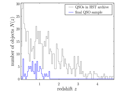
In order to identify our objects and find their redshifts, we searched the NASA Extragalactic Database (NED) for objects of type “QSO” near each set of coordinates, taking the redshift of the closest match ($93\%$ were found). We next eliminated all observations that did not cover the objects’ redshifted Lyman- wavelength (calculated from the NED redshift), which excluded about $44\%$ of the objects. We found additional spectral datasets for these same objects by searching MAST for observations at the coordinates of the already-identified objects, then selecting additional spectra containing the Lyman- line. We eliminated all observations that were not taken with a grating (i.e. prism or mirror observations). At this point we ran our code to align and coadd the selected spectra, as described in Appendix A. We then eliminated spectra that did not include a designated wavelength range surrounding the line ($1200$–$1286$ Å rest frame, cutting the object list by another $15\%$), and excluded spectra with a mean signal-to-noise ratio of less than 10 (eliminating $42\%$ of the remaining objects). This left 120 spectra of 112 objects (only one GHRS spectrum, the rest FOS). After running our line-profile fits, we eliminated 16 more spectra (14 objects) for which our line-profile fitting code failed to converge (usually in the emission/absorption feature detection stage; see Appendix B). After visual inspection of the full-profile fits we cut 21 more spectra (20 objects), 8 for poor data quality (obvious bias in the flux over part of the wavelength range, for instance), 2 because the spectra lacked visible emission features, and 11 because of excessive absorption, either in the form of Lyman- forest lines or broad absorption lines. This left 86 spectra (all FOS) of 78 objects as our final sample. Table 1 lists all 120 automatically-selected spectra, with notes on the 21 spectra that were cut, as well as on other unusual spectra or fits. Figure 1 shows the redshift distributions of all of the quasars found in the HST archives, and of those selected for this project. We have not, so far, used any Space Telescope Imaging Spectrograph (STIS) data, but this would increase our sample considerably (perhaps by a factor of two).

Table 1: HST (FOS and GHRS) quasar Lyman- emission line spectra.

Name	$z$	Instrument	Aperture	Grating	S$/$N	Comments on spectra
(NED)	(NED)				(mean)	and fits.
3C 273	0.158	FOS	B-2	H13	19.9
[HB89] 1427+480	0.221	FOS	B-3	H13	12.8	Absorption feature in blue wing of the line (flagged in full fit).
PG 0953+414	0.234	FOS	C-2	H13	11.1	Absorption feature at line center.
[HB89] 1156+213	0.349	FOS	B-3	H19	10.7
PG 1049-005	0.360	FOS	C-2	H19	13.6	Excluded due to bad blue edge of spectrum.

The name and redshift $z$ are from NED. This is a sample of the full table, which is available in the electronic version.

Figure 1: Redshift distribution of the sample. The upper (grey) line shows all of the NED redshifts we found for quasars in the MAST Hubble archive. The lower (blue) line is for the sample of 87 spectra we adopted for this project (see §2.1).

2.2 Defining a spectral model

In order to characterize the uncertainties inherent in extrapolating a high-redshift quasar’s spectrum from the red side of the Lyman- line to the blue side, we performed two kinds of fits on our low-redshift spectra: one using the full profile visible in the low-$z$ spectra, and one using only the data from the red side of the line (mimicking a fit to a high-$z$ spectrum).

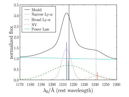
We follow MH07 and adopt the commonly-used spectral model consisting of a power-law continuum, a Gaussian N v line, and a double-Gaussian Lyman- line. Although the N v line is actually a doublet ($1238.821$ and $1242.804$ Å), we fit it with a single Gaussian since the lines are quite broad and thoroughly blended. On the other hand, the Lyman- line usually has prominent broad and narrow components in quasar spectra (thought to arise from gas close to, and relatively farther from the central black hole, respectively), so we fit it with two independent Gaussians. Note that the components found in our fits do not necessarily correspond to physically distinct emission regions, but this combination does yield good phenomenological fits to the line profiles, which is our primary concern in this paper.

Our spectral model, illustrated by the best-fit to a typical spectrum (the quasar 3C 273) is shown in Figure 2. The line centers of the three Gaussians, especially that of the narrow Lyman- component, are shifted significantly from their nominal wavelengths (as discussed in §3.2). The model has three parameters for each Gaussian (width, central wavelength, amplitude) and two for the power-law (index and normalization), for a total of 11 free parameters. In practice, the power-law is fit first, then a separate fit is performed with the power-law parameters fixed and the emission line parameters free. In some fits the power-law index or line centers are also fixed (see §3 and 4).

Figure 2: A model for a quasar spectrum (3C 273) in the vicinity of the Lyman- emission line. Components (as given in the legend) are: broad and narrow Lyman- Gaussians, a N v Gaussian, and a power-law continuum. The centers of the Gaussian components (which are shifted significantly relative to their nominal wavelengths based on the NED redshift) are indicated with short vertical lines. Complete vertical lines indicate the nominal central wavelengths of Lyman- (solid) and N v (dotted).

2.3 Procedure for line-profile fitting

Each fit is performed using Levenberg-Marquardt $\chi^{2}$ minimization. We perform our fits separately for the continuum and the combined emission lines. First we fit the power-law alone to regions of the spectrum chosen to be free of emission features. The power-law fit regions are, in the rest frame: $[1155,1165]$, $[1280,1293]$, $[1315,1325]$, and $[1340,1360]$ Å. Some spectra do not include this full wavelength range. In any fit to a spectrum that lacks data at $\lambda_{0}<1165$ Å we fixed the power law index to $-1.3$, since we have found that extrapolating the continuum from only the longer-wavelength regions can be unreliable.

Once the index and normalization of the power-law are determined and fixed, the emission line components are fit to a region centered on the Lyman- line at $1215.67$ Å, plus two neighboring continuum-dominated regions. The continuum regions are included to help constrain the widths of extremely broad Gaussian components. The Gaussian fit regions are, in the rest frame: $[1155,1165]$, $[1185,1250]$, and $[1280,1293]$ Å.

Initial values for the model parameters are given below. These were chosen by trial and error to speed convergence, and are not necessarily representative of the best-fit values. The powerlaw index and normalization start at

$$p=-1.3;\\ a_{\mathrm{p}}=\tilde{F}_{\mathrm{PL}},$$ (1)

where $\tilde{F}_{\mathrm{PL}}$ is the median flux in the power-law fit region and the continuum flux is given by

$$F_{\lambda}=a_{\mathrm{PL}}\left(\frac{\lambda}{\lambda_{0}}\right)^{p},$$ (2)

with $\lambda_{0}=1215.67(1+z)$ Å. The Lyman- narrow-component width, center, and amplitude start at

$$\sigma_{\mathrm{L\upalpha 0}}=4~{}(1+z)~{}\mathrm{\AA};\\ \mu_{\mathrm{L\upalpha 0}}=1215.67~{}\mathrm{\AA};\\ a_{\mathrm{L\upalpha 0}}=\tilde{F}_{\mathrm{G}}.$$ (3)

The Lyman- broad-component width, center, and amplitude start at

$$\sigma_{\mathrm{L\upalpha 1}}=8~{}(1+z)~{}\mathrm{\AA};\\ \mu_{\mathrm{L\upalpha 1}}=1215.67~{}\mathrm{\AA};\\ a_{\mathrm{L\upalpha 1}}=\tilde{F}_{\mathrm{G}}.$$ (4)

The N v width, center, and amplitude start at

$$\sigma_{\mathrm{NV}}=2~{}(1+z)~{}\mathrm{\AA};\\ \mu_{\mathrm{NV}}=1240.81~{}\mathrm{\AA};\\ a_{\mathrm{NV}}=2\tilde{F}_{\mathrm{G}},$$ (5)

where $z$ is the redshift of the quasar (from NED), $\tilde{F}_{\mathrm{G}}$ is the median flux in the Gaussian fit region, and the flux for Gaussian component $i$ is given by

$$F_{\lambda,i}=a_{i}\exp{\left[\frac{-(\lambda-\mu_{i})^{2}}{2\sigma_{i}^{2}}\right]}.$$ (6)

While we chose to use low-redshift quasars in order to study relatively unobscured spectra, some absorption features do appear from both the Galactic interstellar medium (ISM) and the IGM. In order to avoid ISM absorption lines, we exclude a small region around all of the lines listed by Verner, Barthel & Tytler (1994). The half-width of the excluded region is given by $w=\sqrt{w_{\mathrm{min}}^{2}+w_{\mathrm{Inst}}^{2}}$, where $w_{\mathrm{min}}=1.5$ Å and $w_{\mathrm{Inst}}=2~{}\mathrm{FWHM}/2.355$, with $\mathrm{FWHM}$ being the full width at half maximum of the instrumental line spread function (LSF).

We use an iterative scheme described in Appendix B to exclude other absorption features. In order to avoid biasing the results, we apply essentially the same exclusion criteria to positive and negative deviations, meaning we exclude both excess absorption and emission. In practice very few pixels are flagged as emission features (except for some spectra in which broad emission lines intrude into the power-law fit regions), while most absorption features obvious to the eye (or in the ISM list) are flagged, with few apparently spurious detections. Once this feature detection scheme converges, we perform a final fit on the masked spectrum to determine the best-fit parameters.

3 The Shapes of Low-$z$ Quasar Line Profiles

3.1 Quality of the line-profile fits

Figure 3: Spectral model fit to the observed spectrum of 3C 273 using the full line profile (top plot) and using only data redward of Lyman- (bottom plot). The points in the upper panels show the observed flux ($\mathrm{erg~{}s^{-1}~{}cm^{-2}~{}\AA^{-1}}$), with error envelope in grey. The best-fit model is the black line (often hidden by the data). Vertical solid (green) lines indicate expected broad emission lines (at the quasar redshift), while vertical dashed (purple) lines indicate expected narrow ISM absorption lines (at $z=0$). Red points were used for the power-law continuum fit. Blue points were used for the line-profile fit. Green points were excluded because of the presence of absorption lines. Grey points were not included in the fit. The top axis is labeled in the quasar rest frame, the bottom in the observer frame. The bottom panels show the residuals divided by the quoted formal measurement error. At the bottom-right are sideways histograms of the residuals (points) with the expected Normal distributions shown by the solid lines. The text in the upper panels gives the redshift $z$; the widths $\sigma$ of the narrow Ly-, broad Ly-, and N v components; the height of each component relative to the continuum $a/a_{\mathrm{p}}$; the velocity shifts $v_{\mathrm{shift}}$ of each component; the powerlaw index $p$; the continuum amplitude at Ly- line center $a_{\mathrm{p}}$ ($\mathrm{erg~{}s^{-1}~{}cm^{-2}~{}\AA^{-1}}$); and the reduced $\chi^{2}$ values $\chi^{2}/\nu$ for the continuum and line-profile fits, respectively.

Table 2: Quasar Emission Lines Near Lyman-

Line	Rest-Frame Wavelength
	$\lambda_{0}$ (Å)
C iii*	1175.70
Lyman-	1215.67
N v	1238.82
N v	1242.80
Si ii	1262.59
O i+Si ii	1305.53
C ii	1335.31
Si iv+O iv]	1399.80

Wavelengths are from the SDSS Reference Line List (http://www.sdss.org/dr6/algorithms/speclinefits.html) with Si ii and C iii* from Vanden Berk et al. (2001) and N v doublet from the Atomic Line List (http://www.pa.uky.edu/~peter/atomic/) compiled by Peter van Hoof.

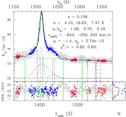
Before proceeding to our main goal of studying the impact of emission-line shape variations of fits to high-$z$ quasars, in this section we describe how well the full profiles can be fit with our adopted spectral model. An example of a typical fit to a quasar spectrum is shown in Figure 3 (top plot). The upper panel shows the spectrum, while the lower panel shows the residuals. Pixels included in the fits are shown as colored points (red for the continuum fits and blue for the line-profile fits). The model spectrum (black solid line, almost entirely hidden by data points) is clearly a good fit to the data used in the fits, as can be seen visually and by the small reduced $\chi^{2}$ values. Vertical solid lines (green) indicate the nominal rest wavelengths (listed in Table 2) of broad quasar emission lines. Vertical dashed lines indicate ISM absorption features listed in Verner et al. (1994). Some of these lines are also visible in the residuals, and these and other pixels excluded from the fits automatically by our absorption-feature detection code are indicated in purple. The bottom-right panel shows sideways histograms of the residuals (blue points for the line-profile fit, red for the continuum fit) with the expected Normal distributions shown by the solid lines, confirming that the distribution of the residuals matches the expected distribution fairly well. The best-fit values of the model parameters are printed on the graph. Table 3 lists the best-fit model parameters for all of the full-profile fits. The amplitudes of the Gaussian components are normalized to the continuum flux at Lyman- (which is stated in the flux units of the spectra, $\mathrm{erg~{}s^{-1}~{}cm^{-2}~{}\AA^{-1}}$). Also given are the reduced $\chi^{2}$ values and the numbers of degrees of freedom for the continuum and line-profile fits.

Table 3: Best-fit spectral parameters from fits to the full line profile.

 
Complete table available in the electronic version.  

The first two columns give the NED name of the target, plus the HST instrument, grating, and aperture used to take the spectrum. $\sigma_{\mathrm{L\upalpha 0}}$ is the width of the narrow Lyman- component (corrected for redshift using the NED value of $z$, see Table 1). $a_{\mathrm{L\upalpha 0}}$ is the amplitude of this component, normalized by the continuum flux $a_{\mathrm{p}}$. $v_{\mathrm{L\upalpha 0}}$ is the shift of the component center from the nominal wavelength calculated with the NED redshift. The next six columns give the same quantities for the broad Lyman- component ($\mathrm{L\upalpha 1}$), and the N v component. $p$ is the continuum power law index, and $a_{\mathrm{p}}$ is the continuum flux at the nominal Lyman- central wavelength, in units of $10^{-15}\mathrm{erg~{}s^{-1}~{}cm^{-2}~{}\AA^{-1}}$. The last columns give the reduced $\chi^{2}$ value $\chi^{2}/\nu$ and the number of degrees of freedom $\nu$ for the continuum and line-profile fits.

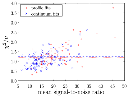
Figure 4 plots the reduced $\chi^{2}$ value, $\chi^{2}/\nu$, for each of our fits versus the mean signal-to-noise ratio for the pixels used in that fit. A large fraction of the fits (41/87 profile and 24/87) are formally unacceptable at the $99\%$ significance level. The $\chi^{2}/\nu$ values corresponding to this significance level (using the median number of degrees of freedom: 183 for continuum and 318 for profile fits) are indicated in the figure by horizontal lines (at $\chi^{2}/\nu=1.26$ and $1.19$ respectively). To the eye, our models generally look like good matches to the overall shape of the line profile. Examination of the residuals suggests that the formally poor fits are due primarily to small deviations at the $\sim 5$–$10\%$ level. This is more than adequate performance for our purposes, but it is interesting to note that the intrinsic quasar spectra are, at some level, more complicated than our models.

Figure 4: Reduced $\chi^{2}$ values versus mean signal-to-noise ratio for the line profile ($+$) and continuum (x) fits. Both values are calculated using only the pixels included in each fit. The $\chi^{2}/\nu$ values corresponding to the $99\%$ significance level (using the median number of degrees of freedom: 183 for continuum and 318 for profile fits) are indicated in the figure by horizontal lines (at $\chi^{2}/\nu=1.26$ and $1.19$ respectively).

3.2 Shifts in Emission Components

Figure 5: Distribution of the shifts of three emission-line components relative to the systemic redshift. Median values are indicated by vertical dotted lines. The median shifts are: $-303~{}\mathrm{km/s}$ for the narrow component, $-413~{}\mathrm{km/s}$ for the broad component, and $-45~{}\mathrm{km/s}$ for the N v component. A handful of extreme values fell outside of the plotted range.

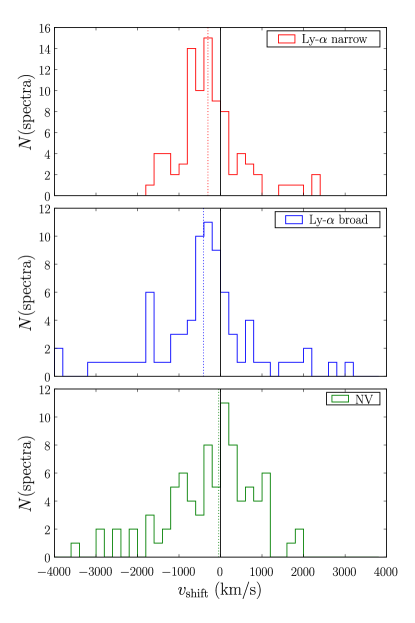
Since our primary concern in this paper is the effect of errors in the extrapolation of intrinsic quasar spectra from the red side of the line to the blue side of the line, we pay particular attention to any shifts or asymmetries in the line profiles that could introduce a systematic bias in the extrapolation. Obviously it is easiest to extrapolate the line profiles from the red side to the blue side if they are symmetric and consistently centered at a well-defined wavelength. Figure 5 shows the distributions of shifts of emission component centers from the fits to all of the spectra. The shifts in the line center wavelength $\mu$ relative to the nominal central wavelength $(1+z)\lambda_{0}$ has been represented as a velocity

$$v_{\mathrm{shift}}=c~{}\frac{\mu-(1+z)\lambda_{0}}{(1+z)\lambda_{0}}$$ (7)

where $z$ is the NED redshift. These shifts are often hundreds or even thousands of $\mathrm{km/s}$, and show little correlation between components. Caution must be exercised in interpreting these velocity values, since our line-profile model is phenomenological rather than physical. Nonetheless, many line profiles clearly show distinct emission components shifted by large velocities relative to their nominal wavelengths and to each other.

The nominal central wavelengths are calculated using the redshifts from NED, which were mostly determined from low-ionization metal lines. It is well known that there is often a velocity offset between high-ionization lines and low-ionization lines in quasar spectra (see discussion and references in Shang et al., 2007). There have been relatively few studies of shifts in the Lyman- and N v lines, in part because of the difficulty of separating the components. Shang et al. (2007) measured velocity shifts of the peak of the Lyman- line relative to the [O iii] $5006.8$ Å line for a sample of nearby quasars ($z<0.4$). This should roughly correspond to our narrow component shifts, since this component dominates in the peak of the overall profile (see Fig. 2). To check this we compared the shifts of line profile peaks versus the best-fit narrow component shift in our sample and found that (with very few exceptions) they indeed correspond closely. Their sample has a mean shift of $-90~{}\mathrm{km/s}$ with standard deviation of $250~{}\mathrm{km/s}$. They also measure the asymmetry of the total line profile, finding that the Lyman- line almost always has an excess in the blue wing, indicating that the broad component tends to be shifted blueward of the narrow component. Their measurements of the shifts of other lines suggest that lines arising from higher ionization states are shifted by larger amounts. Of the lines they measured, they find that the Lyman- shift is well correlated only with the C iv line at $1549.48$ Å.

McIntosh et al. (1999) on the other hand, found a mean velocity shift of $-550~{}\mathrm{km/s}$ between the Lyman- line and the  [O iii] lines for a sample of quasars at $2.0\leq z\leq 2.5$. It is not clear why their distribution is so different, but it may be due to sampling a different population of higher-luminosity quasars (the luminosity limit was $V\leq 18$ versus $B<23$).

There is no consensus on a physical model explaining these shifts, or indeed on a physical model of quasar broad-line and narrow-line regions (BLR and NLR). It has been suggested that the shifts of certain lines may depend on orientation (e.g. Richards et al., 2002) and that there is evidence for a flattened or disc-shaped BLR, with the high-ionization lines being emitted closer to the central black hole (e.g. Decarli et al., 2008). See Marziani et al. (2008) for a review of BLR models. Popović et al. (2004) suggest that there are two components of the NLR, which could explain the blue shift of the Lyman- narrow component relative to the [O iii] lines. In turn, it has been found that the [O iii] line is itself often blueshifted relative to H- (Zamanov et al., 2002) and the [O ii], [N ii], and [S ii] lines (Boroson, 2005).

Regardless of the physical origins of these shifts, we will have understand their effects on the flux extrapolation in order to avoid biasing the IGM measurements from high-redshift spectra. As we discuss in §4 below, these shifts do indeed make it difficult to accurately model the intrinsic spectra of high-redshift quasars. In §6.3 we attempt to correct for the average shifts, but this relies on our knowledge of the intrinsic spectra of low-redshift quasars. Without a clear understanding of the physical origins of these shifts, any attempt to apply a similar correction to the observed population of high-redshift quasars would be highly uncertain. In particular, we worry that the shifts may be correlated with redshift, or with quasar parameters such as luminosity, so that the low-redshift sample is not necessarily representative of the high-redshift population. However, in §6 we show that by careful choice of the wavelength range used in our analysis, we reduce the bias induced by these shifts, and in §6.4 we argue that the sign of the bias actually strengthens current constraints on the IGM neutral fraction.

3.3 Intrinsic asymmetry of the Lyman- emission

Figure 6: Distributions of ratio of red-side to blue-side Lyman- flux. In the top panel the flux is split at $(1+z)\;1215.67$ Å in the observed frame. In the bottom panel the flux is split at the wavelength of the peak of the line. Median values (indicated by vertical dotted lines) are $0.73$ in the top panel and $1.02$ in the bottom. Three extreme values between 2.5 and 7 fell outside of the range plotted in the top panel.

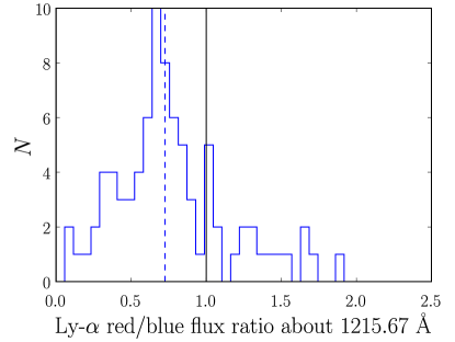
Another way to evaluate the asymmetry of the emission components (in addition to the shifts of the best-fit-model emission components) is to compare the amount of flux on the red and blue sides of the line. Unfortunately, the N v line makes it difficult to do this in a model-independent way, so we rely on our line-profile fits to distinguish between the Lyman- flux and the N v flux. In Figure 6 we plot the histogram of the total flux on the red side of the Lyman- line to the total on the blue side. The flux used is the sum of the narrow and broad Lyman- components from the best-fit model (and therefore excludes the continuum and N v components). A value less than one indicates an overall blueshift of the flux. In the top panel we have divided the flux at the nominal Lyman- wavelength of $\lambda_{0}=1215.67$ Å. As we would expect from the biased distribution of velocity shifts in Figure 5, there is a systematic excess of flux on the blue side of $1215.67$ Å.

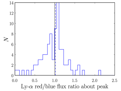
This invites the question of whether the Lyman- profiles are symmetric about some other axis, or are they intrinsically asymmetric? The peak of the line should define the axis of symmetry for a symmetric line profile. The bottom panel of Figure 6 shows the distribution of red-side to blue-side flux split at the wavelength of the peak of the overall line profile. The peak was calculated from the observed spectrum (not the model), by fitting a quadratic to the 10 pixels surrounding the maximum observed flux value and taking the peak wavelength of that function. As mentioned above, this peak corresponds quite closely with the center of the narrow component in all but a few cases (which generally show highly unusual line morphology, often heavily blended with the N v line or having an absorption line near the peak). There is a wide spread in this flux ratio distribution, but it is centered quite close to unity (as measured by both the peak of the histogram and the median value, indicated by the vertical dashed line). On average, the Lyman- emission is symmetric about the peak of the line, but in individual spectra the broad component can be displaced considerably relative to the narrow component, producing an asymmetric total line profile. In the next section we will explore the impact of these shifts and asymmetries on our ability to accurately extrapolate quasar spectra from the red side of the Lyman- line to the blue side.

4 Extrapolating to Obtain the Blue Flux from Fits to the Red Side Alone

In order to mimic fits to high-redshift quasar spectra (which are subject to strong IGM absorption on the blue side of the Lyman- line) we next perform fits using only the spectrum on the red side of the line. Note that actual high-redshift spectra are subject to some additional absorption on the red side of the line due to the IGM damping wing. For simplicity, we do not include the contribution of the damping wing in our continuum fits. In principle, the continuum could always be self-consistently re-estimated for each model hypothesis for the foreground IGM absorption. In practice, the damping wing on the red side is nearly flat (constant with wavelength) and will have a negligible impact on the continuum determination, unless the universe is nearly neutral; furthermore, the continuum is subdominant to the Lyman- emission line at the wavelengths most important for our analysis. In order to make sure to avoid all of the resonant absorption, including from any foreground gas falling towards the quasar that would absorb light on the red side of the line center (Barkana & Loeb, 2003), MH07 excluded not only the blue side of the line profile, but also the peak of the observed line from their line-profile fits. We therefore limit our red-side fits to $\lambda\geq 1220$ Å in the rest frame.

Table 4: Best-fit spectral parameters from fits to the red side only of the Lyman- line.

 
Complete table available in the electronic version.  

The first two columns give the NED name of the target, plus the HST instrument, grating, and aperture used to take the spectrum. $\sigma_{\mathrm{L\upalpha 0}}$ is the width of the narrow Lyman- component (corrected for redshift using the NED value of $z$, see Table 1). $a_{\mathrm{L\upalpha 0}}$ is the amplitude of this component, normalized by the continuum flux $a_{\mathrm{p}}$. $v_{\mathrm{L\upalpha 0}}$ is the shift of the component center from the nominal wavelength calculated with the NED redshift. The next six columns give the same quantities for the broad Lyman- component ($\mathrm{L\upalpha 1}$), and the N v component. $p$ is the continuum power law index, and $a_{\mathrm{p}}$ is the continuum flux at the nominal Lyman- central wavelength, in units of $10^{-15}\mathrm{erg~{}s^{-1}~{}cm^{-2}~{}\AA^{-1}}$. The last columns give the reduced $\chi^{2}$ value $\chi^{2}/\nu$ and the number of degrees of freedom $\nu$ for the continuum and line-profile fits.

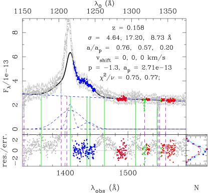
Without the leverage of flux data in the peak and blue wing of the line there is not enough information to simultaneously constrain all three Gaussian parameters for all three components in most cases. We attempted to constrain the full set of line-profile parameters using red-side-only fits, but found that the Gaussian components were often poorly behaved and the resulting best-fit models were too poorly constrained to be useful for extrapolating the flux on the blue side of the line. MH07 avoided this problem by fixing the central wavelength of each component to the nominal wavelength of the line using the systematic redshift determined from metal lines. As we noted above, this is not a reliable assumption, but it is the most reasonable conservative approach, and yielded better matches to the blue-side spectral shapes than fits with free line centers. Similarly, we found that the extrapolation of the continuum to the blue side of the line was more reliable if we fixed the power law index to $-1.3$ in the red-side-only fits (and also in any full-profile fits to spectra lacking coverage at $\lambda_{0}<1165$ Å). Figure 3 (bottom plot) illustrates the type of error introduced by extrapolating the flux using fixed line centers. In this case the observed line profile is shifted blueward by $\sim 600~{}\mathrm{km/s}$. The amplitudes of the Gaussians in the red-side fit with fixed centers are therefore depressed, and the flux is underestimated on the blue side of the line. Table 4 lists the best-fit model parameters for all of the red-side-only fits (see description of Table 3).

Figure 7: Fractional flux excess in the red-side-only fits versus wavelength. The excess is calculated by comparing the red-side-only best-fit model ($F_{\mathrm{ext}}$) to the full-profile fit ($F_{\mathrm{full}}$). The top panel shows the models fit to the full profiles of all 87 spectra (light grey) and the median (dashed) and mean and standard deviation (solid) of the set of model spectra. The bottom panel shows the fractional difference between the models fit to the red side only and the models fit to the full profile for all 87 spectra (light grey), and the median (dashed) and mean and standard deviation (solid) of the fractional flux difference. The vertical solid line (green) indicates the nominal central wavelength of the Lyman- line. The vertical dashed line (blue) at $1220$ Å indicates the blue edge of the red-side-only line profile fit region. The vertical dotted lines at $1199$ Å and $1210$ Å (red) demarcate the typical analysis region for the high-redshift IGM measurements. Note that within this wavelength range the extrapolation is more accurate at shorter wavelengths.

Figure 8: Mean fractional flux excess versus red/blue flux ratio of the Lyman- emission about $1215.67$ Å. The fractional flux excess (see Fig. 7) is averaged over the region between $1199$ Å and $1210$ Å. The distribution of flux ratios is shown in the top panel of Figure 6.

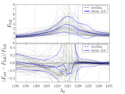
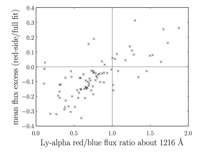
Figure 7 shows the differences between full-profile and red-side-only spectral fits for all 87 spectra. The top panel shows the models fit to the full profiles of each spectrum together with the median, mean, and standard deviation of the set of model spectra. The vertical solid line indicates the nominal central wavelength of the Lyman- line. The mean and median spectra clearly peak a few Å blueward of the nominal rest wavelength. The bottom panel shows the fractional difference between the models fit to the red side only and the models fit to the full profile for each spectrum, together with the median, mean, and standard deviation of the fractional flux difference. The vertical dashed line at $1220$ Å indicates the blue edge of the red-side-only line profile fit region. The agreement between the fits is fairly good on the red side of this limit, as we would expect, since both fits are using the same data here. At shorter wavelengths not only are the differences larger, but there is a bias. The spectra extrapolated from a model fit to the red side only of the Lyman- line tend to systematically underestimate the true spectra.

Both the bias and spread of the flux extrapolation errors vary widely with wavelength blueward of the $1220$ Å lower limit on the red-side-only spectral fits. The core of the Lyman- line is quite poorly predicted from the red-side fits. This is partially because the $1220$ Å lower limit excludes the region where the narrow component dominates, so this component is largely unconstrained in these fits, which is why there is such a large variance in the extrapolation error near line center. The main reason the bias is largest close to the line center (but slightly blueward) is the fact that the line centers are fixed in the red-side fits, while the real lines (and thus the full-profile best-fit models) have emission components that are often shifted by many Å (as we saw in Fig. 5), often to shorter wavelengths. The fixed-center Gaussians in the red-side models can match the red flank of the emission-line fairly well, but once the line starts to peak and turn over somewhere other than $1216$ Å, the quality of the fit has to decline. Specifically, if the real peak of the line is at $\lambda_{0}<1216$ Å, then a Gaussian profile fit to the red side of the line with a center fixed at $1216$ Å will tend to underestimate the flux on the blue side of the peak (as in Fig. 3). This explains why the bias (as measured by the median error spectrum) is close to zero between $1220$ and $1216$ Å, but is largest just blueward of $1216$ Å where most of the observed lines peak. The effect is exaggerated by the fact the line profile is most dominant over the continuum at its peak. The bias is smaller farther to the red where the continuum becomes more and more dominant, indicating that the fixed powerlaw index of $-1.3$ is a reasonable mean value for this sample, though individual spectra still under- and over-estimate the flux by large fractions. The slight positive bias at $\lambda_{0}<1195$ Å is due to the broad C iii emission line at $1175.7$ Å.

The systematic underestimate of the flux by the red-side-only fits will have important consequences for our ability to measure the IGM neutral fraction. The vertical dotted lines at $1199$ Å and $1210$ Å (red) indicate the typical analysis region used for the high-redshift IGM measurements (see §5.2). This IGM analysis range avoids the core of the Lyman- line, where the extrapolation errors are largest but, nonetheless, on average the red-side-only fits underestimate the flux over the entire analysis region. Figure 8 shows the relationship between the mean fractional flux excess in the analysis region and the red/blue flux ratio of the Lyman- emission about $1215.67$ Å. As we expected, red-side-only fits to spectra with blue shifted Lyman- flux tend to underestimate the blue-side flux, and vice-versa. In §6 we explore the possibility of restricting the IGM analysis to $<1205$ Å to reduce the bias, but this obviously also reduces the number of pixels available to analyze. In §6.3 we also attempt to improve on our naive choice of $1216$ Å for the Lyman- line centers with a crude correction for the mean blueshift of the line components, though we caution again that this requires a priori knowledge of (or inferences about) the distribution of line shifts in the high-redshift quasar population.

Our primary concern in this paper is to understand how errors in flux extrapolation like those described above (particularly those caused by the asymmetries in the line profiles) propagate to errors in the final determination of the IGM neutral fraction. In the next section we describe how our line-profile fits are used to simulate high-redshift damping wing measurements in order to evaluate this impact.

5 Simulated high-$z$ damping wing measurements

5.1 Generating simulated high-$z$ quasar spectra

In order to understand how flux extrapolation errors will affect our ability to measure the IGM neutral fraction using the IGM damping wing, we must simulate high-redshift quasar spectra. We begin with the full-profile spectral model fits described in §3. Each best-fit model is used as the intrinsic spectrum of a hypothetical high-$z$ object. We use the line-profile models instead of the actual observed spectra of the low-$z$ quasars so that we can match the expected noise and instrumental resolution of a high-$z$ spectrum. In order to make sure that our flux models capture all of the features relevant to the IGM neutral fraction determination, we also carried out an analysis using the observed spectra (with flagged absorption features, but not emission features, replaced by the model flux values) as the intrinsic spectra of the simulated high-$z$ quasars. We found that the results did not differ significantly from our analysis using the model line profiles as the intrinsic spectra.

We then simulate absorption by neutral hydrogen in the IGM (and instrumental effects) to generate mock absorption spectra on which we can test our techniques for recovering the IGM parameters. We model the density field along lines of sight through the high-$z$ IGM using the probability distribution function (PDF) of Miralda-Escudé, Haehnelt & Rees (2000):

$$P_{V}(\Delta)d\Delta=A\Delta^{-\beta}~{}\exp{\left[\frac{-(\Delta^{-2/3}-C)^{2}}{2~{}(2\delta_{0}/3)^{2}}\right]}d\Delta,$$ (8)

where $\Delta\equiv(\rho/\rho_{0})$ is the density in the IGM normalized by the mean density, and we use the $z=6$ values $A=0.864$, $\delta_{0}=1.09$, $\beta=2.5$, and $C=0.880$ for all of the constants. Our conclusions should be fairly insensitive to small changes in these values, or even in the form of the PDF. The crucial assumption we make is that the density PDF is fairly well known. For actual measurements, uncertainties in the form of the PDF would be an additional source of error that we do not address here.

To construct density profiles $\Delta(r)$ along the line of sight, we generated independent random values of the density from Equation 8 for each patch of IGM. In order to roughly account for photoionization-induced smoothing in the density-field (Gnedin, 2000), we set a minimum co-moving size of $1~{}\mathrm{Mpc}$ on IGM density patches. All pixels falling within the same isodensity patch receive the same IGM density value. We do this in order to avoid having an unrealistically high number of independent data points in our simulated high-resolution spectra. In our mock absorption spectra we have roughly 2 pixels per isodensity patch, and roughly 20 patches are included in each damping-wing analysis. The details of the IGM correlations should not matter a great deal as long as they are short-range (a small fraction of the size of the ionized region), especially since the instrumental FWHM we use is comparable to the isodensity patch size. We have tested this assumption by repeating the analysis with isodensity patches of $0.25~{}\mathrm{Mpc}$ co-moving. The scatter is reduced slightly due to the larger number of independent samples of the optical depth profile, but our overall conclusions are unaffected.

Next we calculate the neutral hydrogen density assuming ionization equilibrium. Three important parameters enter into the calculation at this stage. The ionized region size is $R_{\mathrm{HII}}$. Outside of this region, the ionizing flux is uniform, and is parametrized by $x_{\mathrm{IGM}}$, the equilibrium neutral fraction at mean IGM density. Inside the ionized region, there is additional flux from an ionizing point source (the quasar), parametrized by $x_{\mathrm{ref}}$, which is the equilibrium neutral fraction (including both background and quasar flux) of mean-density gas at a reference point $r_{\mathrm{ref}}=35~{}\mathrm{Mpc}$ comoving away from the quasar.

Physically, the radius $R_{\mathrm{HII}}$ is set by the quasar’s ionizing photon luminosity and its age. The higher the rate of ionizing photon production and the longer the quasar has been shining, the larger its ionized region will be (at least until the recombination rate inside the sphere balances the rate of photon emission, which occurs only at times much longer than the expected quasar lifetime Cen & Haiman 2000). The neutral fraction at a given point inside the ionization front $x_{\mathrm{ref}}$ scales with the luminosity of the quasar.

We define a normalized ionization rate

$$\gamma\equiv\frac{\Gamma}{n_{\mathrm{H}}{}_{B}},$$ (9)

where $\Gamma$ is the number of ionizations per unit time per neutral hydrogen atom, $n_{\mathrm{H}}$ is the total (neutral and ionized) hydrogen density, and ${}_{B}=2.59\times 10^{-13}~{}\mathrm{cm^{3}~{}s^{-1}}$ is the case B recombination coefficient at $T=10^{4}~{}\mathrm{K}$. The normalized background ionization rate required to maintain an equilibrium neutral fraction of $x_{\mathrm{IGM}}$ is then

$$\gamma_{\mathrm{BG}}=\frac{(1-x_{\mathrm{IGM}})^{2}}{x_{\mathrm{IGM}}}.$$ (10)

In order to maintain a neutral fraction $x_{\mathrm{ref}}$ at the reference distance, the additional normalized ionization rate due to the quasar flux must be

$$\gamma_{\mathrm{ref}}=\frac{(1-x_{\mathrm{ref}})^{2}}{x_{\mathrm{ref}}}-\gamma_{\mathrm{BG}}.$$ (11)

Therefore the total ionization rate as a function of luminosity distance from the quasar $r$ (inside the ionized region), is

$$\gamma(r)=\frac{\bar{n}_{\mathrm{H}}(r_{\mathrm{ref}})}{n_{\mathrm{H}}(r)}\left[\gamma_{\mathrm{ref}}\left(\frac{r_{\mathrm{ref}}}{r}\right)^{2}+\gamma_{\mathrm{BG}}\right],$$ (12)

where the ratio of the mean IGM hydrogen density at $r_{\mathrm{ref}}$ to the local hydrogen density at $r$ is given by

$$\frac{\bar{n}_{\mathrm{H}}(r_{\mathrm{ref}})}{n_{\mathrm{H}}(r)}=\Delta(r)^{-1}~{}\left[\frac{1+z(r_{\mathrm{ref}})}{1+z(r)}\right]^{3}.$$ (13)

This factor simply compensates for the fact that $\gamma_{\mathrm{ref}}$ and $\gamma_{\mathrm{BG}}$ are defined with reference to the mean IGM density at $r_{\mathrm{ref}}$. Outside the ionized region ($r>R_{\mathrm{HII}}$), the quasar contribution is zero ($\gamma_{\mathrm{ref}}=0$), so the ionization rate is simply

$$\gamma(r)=\frac{\bar{n}_{\mathrm{H}}(r_{\mathrm{ref}})}{n_{\mathrm{H}}(r)}\gamma_{\mathrm{BG}}.$$ (14)

The equilibrium neutral fraction at distance $r$ from the quasar is

$$x(r)=\frac{-b-\sqrt{b^{2}-4}}{2},$$ (15)

with

$$b=-2-\gamma(r).$$ (16)

Finally, the optical depth due to resonant absorption is (Miralda-Escudé, 1998)

$$\tau_{\mathrm{r}}(\lambda)=\tau_{0}~{}x(r)\left[\frac{\Omega_{b}h_{0}X}{0.03}\right]\left[\frac{H_{0}(1+z)^{3/2}}{H(z)}\right]\left[\frac{1+z}{6}\right]^{3/2},$$ (17)

where $\tau_{0}=2.1\times 10^{5}$, $r$ and $z$ are the distance and redshift corresponding to wavelength $\lambda$, $H(z)$ is the Hubble constant at redshift $z$ (see, e.g. Hogg, 1999), and $h_{0}=H_{0}/100~{}\mathrm{km~{}s^{-1}~{}Mpc^{-1}}$. We use $\Omega_{b}=0.0462$, $\Omega_{c}=0.233$, $\Omega_{\Lambda}=0.721$, $\Omega_{m}=\Omega_{c}+\Omega_{b}$, $\Omega_{k}=0$, $h_{0}=0.701$, and the hydrogen fraction $X=1-0.240$ (Komatsu et al., 2008).

Inside the transmission window in the quasar spectrum (corresponding to the ionized region), at wavelength $\lambda$ there is both resonant absorption $\tau_{\mathrm{r}}$ by hydrogen at $z=\lambda/\lambda_{0}-1$, and absorption by the extended damping wing $\tau_{\mathrm{d}}$ of hydrogen at lower redshifts in the Gunn-Peterson trough. We calculate $\tau_{\mathrm{d}}$ using an analytical expression for the red wing of the GP trough derived by Miralda-Escudé (1998, equations 11 and 12).

The total optical depth inside the transmission window is the sum of the resonant contribution from the residual neutral hydrogen inside the ionized region, and the damping wing absorption from the hydrogen in the IGM,

$$\tau(\lambda)=\tau_{\mathrm{r}}(\lambda)+\tau_{\mathrm{d}}(\lambda),$$ (18)

and the transmitted flux is

$$F_{\mathrm{obs}}(\lambda)=F_{\mathrm{i}}(\lambda)e^{-\tau(\lambda)},$$ (19)

where $F_{\mathrm{i}}(\lambda)$ is the intrinsic spectrum of the quasar.

Finally, we smooth the mock spectrum with an instrumental line spread function and add noise. We use a spectral resolution of $R=2000$. The spectrum is smoothed by Gaussian convolution with a kernel of width $\sigma_{\mathrm{LSF}}=\lambda_{0}(1+z)/(2.355~{}R)$. The pixel size is $\Delta\lambda=\lambda_{0}(1+z)/(2.5~{}R)$. We normalize the spectral models to have the same intrinsic continuum flux $F_{0}$ at $\lambda_{0}$. Our noise model, chosen by hand to mimic a typical spectrum of a high-$z$ quasar (Fan et al., 2006), is a combination of a shot-noise term and a constant background term, giving flux variance (in normalized units) $\sigma_{F}^{2}(\lambda)=e_{F}^{2}F(\lambda)+e_{\mathrm{BG}}^{2}$ with $e_{F}=10^{-2}$ and $e_{\mathrm{BG}}=10^{-3}$. This rough, order of magnitude estimate of the noise level suffices, since, in practice, instrumental noise has very little impact on the fits due to the much larger fluctuations in the observed flux caused by density variations in the IGM.

Figure 9: Generating a mock absorption spectrum: density (top), optical depth (middle), and flux (bottom) profiles along the line of sight to a hypothetical $z=6.28$ quasar. The top panel shows the total ($\rho_{\mathrm{H}}$, black) and neutral ($\rho_{\mathrm{HI}}$, blue dotted) hydrogen density normalized to the mean density of the IGM. The model parameters are $R_{\mathrm{HII}}=40.5~{}\mathrm{Mpc}$, $x_{\mathrm{ref}}=10^{-5.5}$, and $x_{\mathrm{IGM}}=0.1$. The middle panel shows the damping wing and resonant optical depths, and their sum. The extreme optical depths in the Gunn-Peterson trough (at $\lambda\la 8730$ Å) are above the range of this plot. The bottom panel shows a model intrinsic spectrum (dotted) and mock absorption spectrum (solid black). A Keck spectrum of the $z=6.28$ quasar J1030+054 (grey) is also shown (Becker et al., 2001). Note that the model was not fit to this spectrum, it is shown merely for comparison.

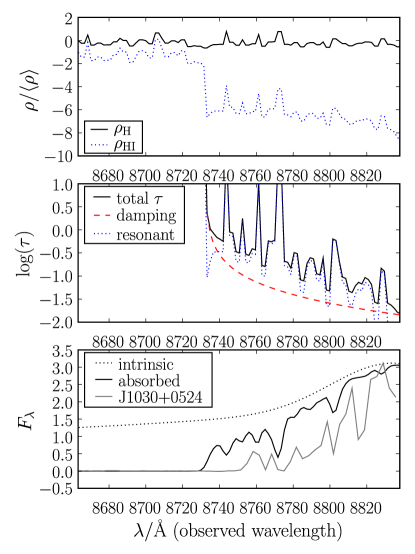
Figure 9 shows the density, optical depth, and flux profiles for a model high-redshift quasar. The effects of both the uniform ionizing background and the quasar flux are evident in the deficit in the neutral hydrogen density relative to the total hydrogen density. The optical depth is much lower inside the ionized region, allowing the quasar flux to reach us. With these parameters, the resonant absorption dominates the opacity in high-density regions, while the damping wing dominates in low-density regions, setting an effective optical depth floor. The plot of the spectrum (in the bottom panel) demonstrates that the transmission window is superimposed on the blue wing of the quasar’s intrinsic Lyman- line. The flux is entirely absorbed in the Gunn-Peterson trough (at $\lambda\la 8730$ Å), but a large fraction is transmitted in the wavelength range corresponding to ionized region. The Keck spectrum of the $z=6.28$ quasar J1030+054 is qualitatively quite similar, differing mostly in that the transmission window is slightly smaller and instrumental broadening has smoothed the flux variations somewhat.

5.2 Analysis of the mock spectra

In order to test the impact of intrinsic Lyman- line shape variations on the recovery of IGM and H ii region parameters from a high-$z$ quasar spectrum, we implement a version of the method used by MH07. The first step is to extrapolate the flux by fitting a spectral model to the red side of the Lyman- line, as described in §2.3. We then calculate the optical depth by comparing the extrapolated spectrum to the mock absorption spectrum and solving equation 19 for the optical depth, substituting the extrapolated flux $F_{\mathrm{fit}}$ for the intrinsic flux and the observed flux $F_{\mathrm{obs}}$ for the transmitted flux:

$$\tau_{\mathrm{obs}}=\ln\left(\frac{F_{\mathrm{fit}}}{F_{\mathrm{obs}}}\right).$$ (20)

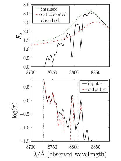
An overestimate of the intrinsic flux results in an overestimate of the optical depth, and vice-versa. Figure 10 illustrates this effect. The top panel shows the intrinsic spectrum of a mock high-redshift quasar (based on the observed spectrum of 3C 273), the mock spectrum after absorption in the IGM, and the flux extrapolated from a fit to only the red side of the Lyman- line. It can be seen that the flux extrapolated from red-side-only fit in this case (as is typical) underestimates the intrinsic spectrum of the model quasar. When the extrapolated flux is used to calculate the optical depth profile (shown in the bottom panel), the error in the flux extrapolation results in errors in the inferred optical depth profile. Within the analysis region typically used for high-redshift IGM measurments ($1199$–$1210$ Å in the rest frame), there is a systematic underestimate of the optical depth which is largest at longer wavelengths, where the extrapolation error is largest. Note that there are regions of the spectrum where the absorbed flux exceeds the extrapolated flux by significant fraction. This is outside of the line-profile fit region as we have defined it here for high-$z$ fits ($\lambda_{0}>1220$ Å), but in principle observed absorbed flux values on the blue side of the line could be included in the fits as lower limits on the intrinsic flux, which would decrease the underestimate of the flux somewhat.

Figure 10: Error in the mock “observed” optical depth profile: Flux (top) and optical depth (bottom) on the blue side of the Lyman- line. The top panel shows the intrinsic (unabsorbed) flux, flux extrapolated from the red-side fit, and mock absorption spectrum for a model quasar at $z=6.28$ (based on the observed spectrum of 3C 273). The bottom panel shows the input model optical depth (used to generate the spectrum), and the output optical depth inferred by comparing the mock absorption spectrum and the extrapolated flux. The mismatch between these lines is caused by the mismatch between the intrinsic spectrum of the quasar, and the spectrum extrapolated from a fit to the red side of the Lyman- line. The vertical dotted lines (at $1199$ Å and $1210$ Å in the quasar rest frame) indicate the typical analysis region for the high-redshift IGM measurements.

Once we have an optical depth profile, we need to fit a model to it to recover our parameters of interest. Because the density fluctuations in the IGM cause large flux variations, this is not a trivial task. MH07 solved the problem by grouping the flux values into three wavelength bins, then using the Kolmogorov-Smirnov (K-S) test to compare the distribution of flux values in each bin with a distribution derived from simulations. The product of the three K-S probabilities $p$ then served as the relative likelihood estimate for that combination of parameters. They then compared observed quasars to a grid of models using this technique, selecting the model with the maximum $p$-value as the best fit. Optical depth values above about $6$ are not measurable from a real spectrum because the flux drops below the detection limit. We therefore set any $\tau>6$ to $\tau_{\mathrm{max}}=6$. Note that the K-S test is not strictly valid with censored data, and assumes all values are independent, neither of which holds in this case. Therefore care must be taken in interpreting the $p$-values. We rely on Monte-Carlo simulations to avoid depending on the $p$-values to determine confidence intervals.

We will distinguish between our grid of “model” optical depth profiles, used to make the canonical distributions for the K-S test, and our set of “mock” profiles, which we are analyzing as if they were observed high-$z$ quasars, even though they are all generated using the same techniques outlined above. The only difference is that the model optical depth profiles are generated without reference to a spectrum, while the mock profiles use the extrapolated spectra, and thus incorporate any errors in the flux extrapolation.

At each point in our parameter-space grid we generate 100 model profiles, and we use each real low-$z$ quasar spectrum to generate $200$ mock optical depth profile observations using a single set of input parameters, making a total of $86\times 200=17200$ mock profiles. We then run the optical depth analysis on each mock spectrum, and track the distribution of the recovered best-fit parameters $(R_{\mathrm{HII}},x_{\mathrm{ref}},x_{\mathrm{IGM}})$.

By default, the maximum wavelength of the analysis range is $\lambda_{\mathrm{max}}=1210$ Å in the rest frame. MH07 excluded pixels closer to the Lyman- line center to avoid the biased environment close to the quasar. This has the added advantage of avoiding the most problematic area for flux extrapolation — the narrow-component-dominated core of the line (since the narrow component is less well constrained in the line profile fits and is affected more by shifts in the line center). The minimum wavelength is chosen by finding the bluest pixel with $\tau\leq 6$, then extending the overall wavelength range blueward by $5\%$. The inclusion of these extra “dark” pixels is important for the statistical comparison with mock spectra, since density variations change the exact wavelength at which the optical depth exceeds $\tau=6$ for different spectra with the same value of $R_{\mathrm{HII}}$. With $R_{\mathrm{HII}}=40.5~{}\mathrm{Mpc}$, the typical range is roughly $1199$–$1210$ Å, divided evenly into three bins of about $15$ pixels each.

6 The Impact on Parameters Estimated from High-$z$ Spectra

6.1 Parameter Recovery with Known Intrinsic Spectra

Figure 11: Parameter recovery map using perfectly known intrinsic spectra. Each panel is a slice through parameter space. The shading of each square indicates the number of best-fit values that fell within that cube in parameter space (darker indicates larger numbers). The input parameters ($R_{\mathrm{HII}}=40.5\ \mathrm{Mpc}$, $x_{\mathrm{ref}}=10^{-5.5}$, $x_{\mathrm{IGM}}=0.1$) are indicated with a white point. The top group of graphs show slices of constant H ii region radius. The middle group shows slices of constant internal reference neutral fraction. The bottom group shows slices of constant IGM neutral fraction. Note that the distribution peaks at the correct values, however there is a large scatter induced by density fluctuations along the line of sight.

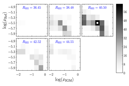
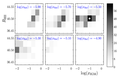
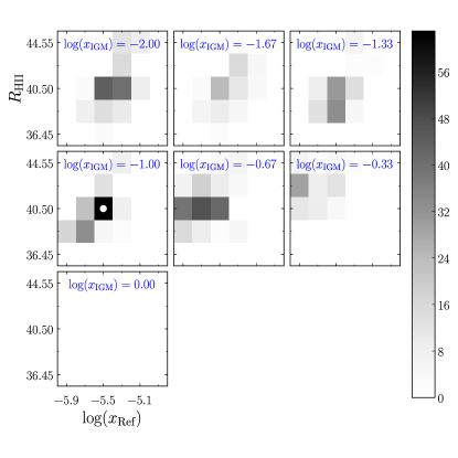
In order to test recovery of IGM parameters without extrapolation errors, as a sanity check we first calculate a set of mock optical depth profiles using the “correct” intrinsic model spectra in Equation 20 instead of the extrapolated spectra $F_{\mathrm{fit}}$. We then analyze the profiles as described above. We used only 4 different intrinsic spectral models (chosen at random from our set of full-profile fits) for this purpose, since the shape of the underlying spectrum has little impact on the parameter recovery if it is perfectly known. Figure 11 shows the distribution of the best-fit values from the 800 mock optical-depth fits in our 3-dimensional parameter space (200 random IGM density profiles times 4 intrinsic spectra). The input parameters are $R_{\mathrm{HII}}=40.5~{}\mathrm{Mpc}$; $x_{\mathrm{ref}}=10^{-5.5}$; $x_{\mathrm{IGM}}=0.1$. The shading of each square indicates the number of best-fit values that fell within that cube in parameter space (darker shading indicates larger numbers). The top group of graphs show slices through our parameter space in planes of constant $R_{\mathrm{HII}}$. The middle group shows slices of constant $x_{\mathrm{ref}}$. The bottom group shows slices of constant $x_{\mathrm{IGM}}$. The regions of darker shading trace out degeneracies between all of the parameters, which are easily understood. Increasing either $x_{\mathrm{IGM}}$ or $x_{\mathrm{ref}}$ increases the optical depth, so these parameters are anti-correlated (top group of graphs). When the best-fit value of the IGM neutral fraction is overestimated, the internal neutral fraction tends to be underestimated. On the other hand, increasing $R_{\mathrm{HII}}$ moves the damping wing away from a given wavelength coordinate and decreases the optical depth, so the ionized region radius is positively correlated with the other two parameters (middle and bottom groups of graphs).

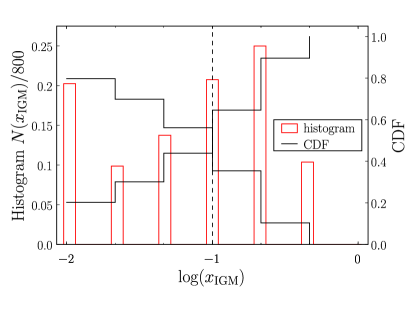
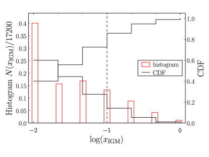
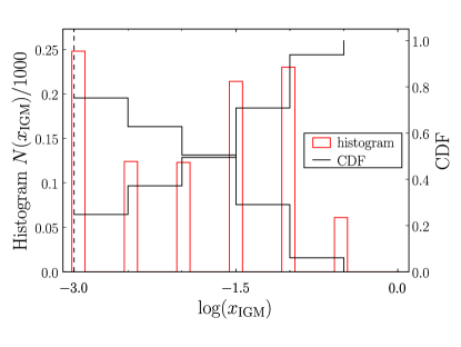
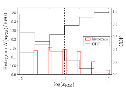
The density fluctuations along the line of sight induce a wide scatter in the recovered values, which follows the degeneracy contours we described above. Even so, the distribution of best-fit parameters in Figure 11 is peaked at exactly the coordinates of the input parameters. The top panel of Figure 12 shows the marginalized distribution of recovered $x_{\mathrm{IGM}}$ values. Black lines show the cumulative distribution function (CDF) and its complement. Where they cross (at $50\%$) is the median value. While the marginalized distribution peaks slightly above the input value, the median recovers the input value (indicated by the vertical dashed line) exactly. The secondary peak at $\log(x_{\mathrm{IGM}})=-2.0$ represents the integral of the long negative tail of the distribution which is truncated by our finite logarithmic grid (which we must keep small for computational speed).

Because of our coarse parameter-space grid it is difficult to quote conventional confidence limits, but we can see from Figure 12 that $80\%$ of the marginalized neutral fraction distribution is in the interval $\log(x_{\mathrm{IGM}})=-1.0\pm 0.6$, $90\%$ of the distribution is at $x_{\mathrm{IGM}}\leq 0.22$, and $100\%$ at $x_{\mathrm{IGM}}\leq 0.46$ (none of the 800 best-fit values implied a neutral IGM). Similarly, $88\%$ of the internal reference neutral fraction values (distribution not shown) are in the interval $\log(x_{\mathrm{ref}})=-5.5\pm 0.2$, and $93\%$ of the HII region radii are within $R_{\mathrm{HII}}=40.5\pm 2~{}\mathrm{Mpc}$ (the distributions of both of these parameters peak and have their median at the input value). These represent the approximate confidence limits that could be placed on these parameters from a single high-$z$ quasar spectrum in the limit of perfect knowledge of the intrinsic quasar spectrum, the density distribution in the IGM, and the radial profile of the background ionizing flux. We find similar results in simulations with $x_{\mathrm{IGM}}\approx 0.2$ and known intrinsic spectra. For instance, $98\%$ of the results are at $x_{\mathrm{IGM}}\leq 0.46$ in that case.

Figure 12: Marginalized distribution of estimated $x_{\mathrm{IGM}}$ values with perfectly known (top) and extrapolated (bottom) intrinsic spectra. The histogram (axis scale on the left) shows the marginalized distribution of recovered $x_{\mathrm{IGM}}$ values. Black lines show the cumulative distribution function (CDF), i.e. the fraction of recovered values at $x<x_{\mathrm{IGM}}$ (increasing curve, axis scale on the right) and its complement (decreasing curve). Input parameters are $R_{\mathrm{HII}}=40.5~{}\mathrm{Mpc}$, $x_{\mathrm{ref}}=10^{-5.5}$, $x_{\mathrm{IGM}}=0.1$. The vertical dashed line indicates the input value. The median value occurs where the CDF and its complement cross.

6.2 Parameter Recovery with Extrapolated Intrinsic Spectra

Figure 13: Parameter recovery map using mock spectra with unknown intrinsic spectra. The shading of each square indicates the number of best-fit values that fell within that cube in parameter space. The input parameters ($R_{\mathrm{HII}}=40.5\ \mathrm{Mpc}$, $x_{\mathrm{ref}}=10^{-5.5}$, $x_{\mathrm{IGM}}=0.1$) are indicated with a white point. Compare with Figure 11, which has the same input parameters but uses known intrinsic quasar spectra: an additional scatter, as well as a bias has been induced by errors in the extrapolation of the intrinsic spectrum.

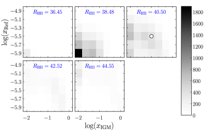
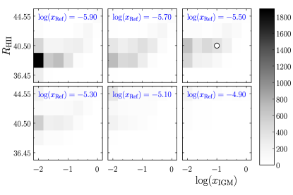
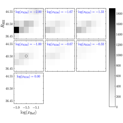
In order to understand the effect that flux extrapolation errors have on the recovered parameters, we tested IGM parameter recovery using our more realistic mock optical depth profiles, calculated using the spectra extrapolated from the red side of the line profile. This mimics the process of obtaining such a profile from a high-$z$ quasar spectrum, where the intrinsic flux is unknown. The distribution of $17200$ best-fit values ($86$ observed spectra times $200$ random density profiles) from the optical depth analysis using these profiles is shown in Figure 13. The same degeneracies as in Figure 11 (with known spectra) are evident, but the peak of the distribution has shifted to the minimum values of the internal and external neutral fraction, and to a lower value of the H ii region radius. Figure 12 compares the marginalized distributions of recovered $x_{\mathrm{IGM}}$ values with known and with extrapolated intrinsic spectra. Both the median and peak of the distribution have moved to lower values, and the “secondary” peak at $x_{\mathrm{IGM}}=-2.0$, representing the integral of the tail of the distribution that would extend to lower values if not truncated by our finite logarithmic grid, now contains $40\%$ of the results.

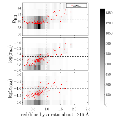
This bias in the fits toward underestimating the true neutral fraction is caused by the bias in the flux extrapolation that we discussed in §3. This can be seen in Figure 14, where we plot the recovered IGM parameters versus the red-to-blue flux ratio about $1215.67$ Å. The shading shows the 2D distribution of all $17200$ fit results. The points show the mean value for each of the $86$ intrinsic spectral models (over 200 random density profiles). There are obvious correlations between the flux ratio and each of the fit parameters. Because there are more spectra with excess blue flux than excess red flux (Fig. 6), and because the red-side-only fits tend to underestimate the blue-side flux of spectra with blue-shifted Lyman- lines (Figures 7 and 8), there are more red-side fits that underestimate the flux than overestimate it. If the intrinsic flux is underestimated, then the optical depth derived from it will also be underestimated. This tends to favor lower values of the internal and IGM neutral fractions in the optical depth fits, which makes sense, since both parameters correlate positively with optical depth (though the wavelength-dependence of the bias must also play a role in how much each parameter is affected since the components of the optical depth have different profiles). It is a little more surprising that the H ii region radius shows the same sign in the correlation, since it has the opposite relationship with the optical depth. The correlation with the other parameters is apparently strong enough to outweigh the anti-correlation with optical depth.

Figure 14: Best-fit parameters versus the red-to-blue flux ratio of the Lyman- emission about $1215.67$ Å. The shading indicates how many fits fell in a given region of the graph. The red points plot the mean (over 200 random IGM density profiles) of the recovered parameter values for each input spectrum. Input parameters are $R_{\mathrm{HII}}=40.5\ \mathrm{Mpc}$, $x_{\mathrm{ref}}=10^{-5.5}$, $x_{\mathrm{IGM}}=0.1$. See Fig. 6 (top panel) for the distribution of the flux ratio in our sample of spectra.

So far we have tested parameter recovery with the fairly high IGM neutral fraction of $0.1$. In light of the current constraints on the IGM neutral fraction, however, it is interesting to explore the question: how likely is it that an ionized IGM will be mistaken for a neutral IGM? More specifically, what is the probability that the best fit values of $x_{\mathrm{IGM}}=1.0,1.0,0.2$ for three quasars at $z>6.2$ would be obtained (as in MH07) if the IGM were in fact highly ionized? To answer these questions we repeated our analysis with the input neutral fraction lowered to $x_{\mathrm{IGM}}=10^{-3}$.

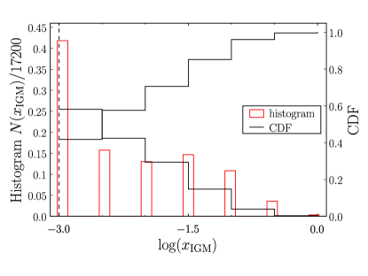
Figure 15 shows the marginalized distributions of recovered $x_{\mathrm{IGM}}$ values with known and extrapolated intrinsic spectra. Even with known intrinsic spectra the median no longer reflects the input neutral fraction. With a highly-ionized IGM the damping wing is too weak to be reliably detected amid the noise of density fluctuations inside the ionized region. We can still place strong upper limits on the neutral fraction, however. With known intrinsic spectra (top panel), none of the best-fit values imply a neutral IGM, $94\%$ of the recovered values were at $\log(x_{\mathrm{IGM}})\leq-0.5$, and $61\%$ at $\log(x_{\mathrm{IGM}})\leq-1.0$. The added errors from using extrapolated spectra actually strengthen the upper limit at some confidence levels due to the bias toward underestimating the neutral fraction. $96\%$ of fits yield $\log(x_{\mathrm{IGM}})\leq-0.5$, and $85\%$ of fits yield $\log(x_{\mathrm{IGM}})\leq-1.0$. The small amount of additional scatter to high neutral fractions is negligible. Only $0.3\%$ of the fits yield a neutral IGM.

Figure 15: Marginalized (over $R_{\mathrm{HII}}$ and $x_{\mathrm{ref}}$) distribution of estimated $x_{\mathrm{IGM}}$ values with perfectly known (top) and extrapolated (bottom) intrinsic spectra, for a highly-ionized fiducial IGM. Input parameters are $R_{\mathrm{HII}}=40.5\ \mathrm{Mpc}$, $x_{\mathrm{ref}}=10^{-5.5}$, $x_{\mathrm{IGM}}=0.001$. Note that the $x$-axis scale extends to lower values than in Fig. 12 because we used a different parameter-space grid.

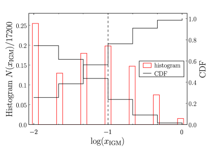
Since the fits tend to perform worse close to the line center, we investigated the potential to reduce the bias by lowering the maximum wavelength of the pixels used in the optical depth fits. This cannot be taken too far, since there are already relatively few pixels used in these fits. Figure 16 shows the results of setting the maximum wavelength of our analysis region to $\lambda_{\mathrm{max}}=1205$ Å rather than $1210$ Å. The fits (using extrapolated spectra) are dramatically improved. The bias is reduced, with the median substantially closer to the input value and the peak of the distribution at the input value. There is a substantial decrease in the scatter toward lower values (only $25\%$ at $\log(x_{\mathrm{IGM}})\leq-2$ versus $40\%$, and only a small increase in the scatter toward high values. Clearly, careful choice of the analysis region can reduce the impact of flux extrapolation errors.

Figure 16: Marginalized recovered $x_{\mathrm{IGM}}$ distribution with the wavelength range of the fit restricted to $\lambda<1205$ Å. Compare to Figure 12 (bottom panel) where $\lambda_{\mathrm{max}}=1210$ Å. The input parameters are $R_{\mathrm{HII}}=40.5\ \mathrm{Mpc}$, $x_{\mathrm{ref}}=10^{-5.5}$, $x_{\mathrm{IGM}}=0.1$ (as in Fig. 12). Lowering the upper limit of the fit range has reduced the bias towards low values of $x_{\mathrm{IGM}}$ at the expense of some extra scatter toward higher values.

6.3 Correcting for Median Line Shifts

Since we have shown that it is the mismatch between the (on average) blueshifted Lyman- emission and the spectral models with line centers fixed at their nominal wavelength that is causing the bias in the optical depth fit parameters (most importantly the IGM neutral fraction $x_{\mathrm{IGM}}$), we decided to attempt to correct for the mismatch by performing red-side-only line profile fits with centers offset by the median shifts found in our full-profile fits. These fits were performed as described in §4, but with velocity offsets fixed at $-303$, $-413$, and $-45~{}\mathrm{km/s}$ for the narrow Lyman-, broad Lyman-, and N v components. Figure 17 (fractional flux excess versus wavelength) confirms that imposing a constant shift at the median value for each component largely eliminates the bias in the flux. As the figure shows, the median flux excess is now close to zero everywhere. There is still a wide scatter, and the mean in fact shows a positive bias in the core of the line. The poor performance in the core is due to the difficulty of constraining the narrow component with the fit range restricted to $\lambda_{0}>1220$ Å, as discussed in §4.

Figure 17: Fractional flux excess in the red-side-only fits (with velocity offsets fixed at their median values) versus wavelength. The excess is calculated by comparing the red-side-only best-fit model ($F_{\mathrm{ext}}$) to the full-profile fit ($F_{\mathrm{full}}$). The top panel shows the models fit to the full profiles of all 87 spectra (light grey) and the median (dashed) and mean and standard deviation (solid) of the set of model spectra. The bottom panel shows the fractional difference between the models fit to the red side only and the models fit to the full profile for all 87 spectra (light grey), and the median (dashed) and mean and standard deviation (solid) of the fractional flux difference. The vertical solid line (green) indicates the nominal central wavelength of the Lyman- line. The vertical dashed line (blue) at $1220$ Å indicates the blue edge of the red-side-only line profile fit region. The vertical dotted lines at $1199$ Å and $1210$ Å (red) demarcate the typical analysis region for the high-redshift IGM measurements. Compare with Figure 17 (which has velocity offsets fixed at zero).

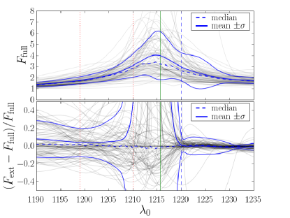
Figure 18 shows the marginalized distribution of recovered $x_{\mathrm{IGM}}$ values using the red-side-only fits with median velocity offsets to extrapolate the intrinsic spectrum. The overall distribution has shifted back toward higher values (closer to the correct input value), correcting the bias somewhat, but the correction is smaller than we might have expected. This crude correction for the median offsets of the emission components is insufficient to eliminate the bias. Interestingly, the peaks and median values of the marginalized distributions for the H ii region radius and internal reference neutral fraction correspond to the input values, so this simple correction has successfully eliminated the bias for these parameters, even though it did not do so for the IGM neutral fraction. It is unclear why this median correction did not eliminate the neutral fraction bias. The most likely explanation is that the neutral fraction is sensitive to the wavelength dependence of the flux extrapolation errors in a way that differs from the other parameters. An additional concern (discussed earlier, in §3.2), is that the distribution of emission-component shifts in the high-redshift quasar population may very well differ from the distribution sampled here. This could mean that the median values for the shifts obtained from this sample (or other low-$z$ samples) would be biased relative to the high-$z$ population. In §7 we discuss more sophisticated techniques for modeling and extrapolating the intrinsic spectrum that should be more successful at eliminating the neutral fraction bias.

Figure 18: Marginalized recovered $x_{\mathrm{IGM}}$ distribution with velocity offsets of the components fixed at their median values. Compare to Figure 12 (bottom panel) where the offsets are fixed at zero. The input parameters are $R_{\mathrm{HII}}=40.5\ \mathrm{Mpc}$, $x_{\mathrm{ref}}=10^{-5.5}$, $x_{\mathrm{IGM}}=0.1$ (as in Fig. 12). Using the median offsets has slightly reduced the bias in the recovered neutral fraction distribution. Compare to Fig. 12, bottom panel.

6.4 Caveats

While our overall conclusion that the bias is in the direction of low $x_{\mathrm{IGM}}$ values should be robust, some caveats apply to the specific numerical results discussed above:

1. These results assume that high-redshift quasars are drawn from the same population of intrinsic spectral shapes as our low-redshift sample. This is probably not a valid assumption in detail, since quasar spectra are known to show luminosity-dependent effects, but it may be a reasonable conservative approximation for our purposes. Studies of the Baldwin effect (Baldwin, 1977; Espey & Andreadis, 1999; Shields, 2007), indicate that the strength of the Lyman- line will decrease relative to the both the N v line and the continuum in more luminous quasars. A quasar 3 orders of magnitude more luminous than the mean for our sample would have a N v equivalent width roughly $50\%$ larger assuming a Baldwin effect slope of $\sim 0.2$ (Espey & Andreadis, 1999), though other measurements indicate a lower value for the slope (0.0 from Dietrich et al., 2002). Similarly, the Lyman- line would be expected to have an equivalent width roughly $30\%$ lower for the same increase in luminosity. This means that the N v line would be up to $2.2$ times stronger relative to the Lyman- line, and the N v line would still contribute no more than a few percent of the flux in the analysis region. Problematic blends with other neighboring lines are similarly unlikely. For instance, the equivalent width of the Si ii line at $1260$ Å shows little dependence on luminosity (Dietrich et al., 2002), so it should still be reliably excluded from our fits. Direct contamination of our analysis region ($1199$–$1210$ Å), would therefore be negligible, even for a relatively enhanced N v line, but one concern is that the more prominent N v line would in some way bias the line profile fits. On the other hand, a stronger N v line could be fit to higher precision, and we have detected no tendency for the N v line shifts to be biased, so this emission component might actually be modeled more accurately using high-luminosity quasar spectra. The fact that the Lyman- line is weaker relative to the continuum in luminous objects should also improve the accuracy of the flux extrapolation, since it is easier to extrapolate the continuum than the line profile, in general. Therefore the simultaneous N v plus Lyman- plus continuum fits may perform better at high redshift. We defer detailed simulation of parameter recovery with high-luminosity spectra to future work. Another concern is that, as we discussed in §3.2, indications are that a high-redshift sample will have larger negative velocity shifts of the Lyman- line relative to the metal lines. Since a larger blueward shift in the line center tends to result in a more severe underestimation of the neutral fraction, the lower limit should still be robust.

2. We assume that the mean IGM density is independent of distance from the quasar over our region of interest (except for the small change in mean density with redshift). As noted by MH07, the exclusion of the $6$–$11$ Å region immediately on the blue side of the nominal line center eliminates the few Mpc region expected to show significant overdensity (Barkana & Loeb, 2004). However, Kirkman & Tytler (2008), Guimarães et al. (2007), and Rollinde et al. (2005) have all inferred large-scale overdensities (on the scale of a few to tens of Mpc) in the IGM from studies of the proximity effect. The ionized regions we are considering are much larger ($\sim 40~{}\mathrm{Mpc}$). However, if the bias did extend into our analysis region, then it would increase the mean density close to the quasar. This differs from an error in the flux extrapolation because it shifts only the resonant contribution to the optical depth. Without detailed study, it is difficult to determine what affect this would have on the neutral fraction measurement. In future work, the density profile can be estimated from numerical cosmological simulations large enough to contain the rare massive host halos of bright quasars. Even if variations in the overdensity around such halos add to the uncertainty in the $x_{\mathrm{IGM}}$ constraint, this should not seriously impact the ability to distinguish highly-ionized and largely-neutral scenarios.

3. We assume that the ionizing background is uniform. In reality the ionizing background arises from a complicated distribution of discrete sources, i.e. galaxies. Inside the large ionized region surrounding a luminous quasar, the background will still be fairly smooth on large scales, since the mean free path of ionizing photons will be large. An overdensity of galaxies would be expected close to the quasar, which would modify the $\tau_{\mathrm{r}}$ curve somewhat (tending to cancel out the effect of the density enhancement described above). If the density of galaxies is enhanced only very close to the quasar (on the order of a few Mpc), then their light will simply add to the quasar flux at larger radii. If, on the other hand, there is a large scale enhancement in the galaxy distribution extending into our analysis region ($~{}\sim 10~{}\mathrm{Mpc}$), then the flux will not fall off like $r^{-2}$, and this would need to be taken into account in future analyses of observed quasar spectra.

4. Outside of the quasar H ii region, reionization of the IGM is expected to occur largely through the growth of discrete ionized bubbles separated by neutral gas. Our expression for the damping wing assumes a uniformly ionized IGM with mean neutral fraction $x_{\mathrm{IGM}}$. If, instead of being spread uniformly along the line of sight, the neutral gas is distributed in a “picket fence” of neutral regions separated by ionized regions, the damping wing will change. Mesinger & Furlanetto (2008) studied this effect using semi-numerical cosmological structure simulations, concluding that, if ignored, this effect biases the recovered neutral fraction by up to $x_{\mathrm{obs}}-x_{\mathrm{IGM}}=0.3$ (where $x_{\mathrm{obs}}$ is the value inferred from observations of the damping wing), and induces a scatter of a similar magnitude (see also, McQuinn et al., 2008). This is in the opposite direction to the bias we find from flux extrapolation errors. However, when Mesinger & Furlanetto (2008) looked specifically at the bias induced by inhomogeneities around the largest halos (the likely hosts of bright quasars) dwelling in large ionized regions, they found that the bias toward overestimation of the neutral fraction was reduced, and even reversed for large neutral fractions, and that the inhomogeneity-induced modification of the damping wing profile may favor underestimation of the neutral fraction. Taking these effects together, a measured value of $x_{\mathrm{obs}}=1$ is still unlikely if $x_{\mathrm{IGM}}\la 0.02$, but more detailed simulation combined with larger quasar samples are needed. Lidz et al. (2007) point out another, related complication. The fluctuations in the ionizing background produce a large scatter and bias in the relationship between the apparent red edge of the GP trough (where the flux drops below some threshold) and the actual location of the ionization front. However this should not affect our method, since we do not assume an $R_{\mathrm{HII}}$ value in order to infer the IGM neutral fraction.

5. We ignore radiative transfer effects, which would be especially important at the edge of the ionized region where the relatively unattenuated flux from the quasar first encounters a significant amount of neutral hydrogen. If the quasar spectrum is hard, the transition region between the highly-ionized interior and the more neutral exterior of the region could be broad enough to modify the observed optical depth profile at the edge of the transmission window (Kramer & Haiman, 2008; Thomas & Zaroubi, 2008). It is unclear what effect this would have on the neutral fraction measurement.

While the caveats listed above will certainly add to the scatter in recovered values, it still seems unlikely that a highly-ionized IGM will be mistaken for a highly-neutral one.

7 Conclusions and Future directions

The main conclusion of this paper is that errors in extrapolating the intrinsic emission line shapes generally cause a bias towards underestimating the $x_{\mathrm{IGM}}$ value; these uncertainties therefore strengthen the conclusions in MH07 about a significantly neutral IGM at $z>6.2$. From the marginalized distributions of recovered IGM parameters shown in the last section, we can see that it is highly unlikely that flux extrapolation errors could cause a highly-ionized IGM to be mistaken for a neutral IGM. If $x_{\mathrm{IGM}}=0.001$, there is less than a $4\%$ chance of inferring $x_{\mathrm{IGM}}\ga 0.3$. Even with $x_{\mathrm{IGM}}=0.1$ there is only a $15\%$ chance of measuring $x_{\mathrm{IGM}}\ga 0.2$ and a $5\%$ chance of measuring $x_{\mathrm{IGM}}\ga 0.4$. Neglecting other sources of error, if the neutral fraction were $\leq 0.1$ there would be less than a $0.04\%$ chance of simultaneously inferring the three best fit values found by MH07.

Besides addressing the caveats mentioned in the last section, there are two basic directions in which we plan to develop this technique in the future. The first is to improve our ability to model and fit the damping wing. This includes improving our modeling of the underlying intrinsic quasar spectra, our models of the optical depth profiles, and the recovery of information from the observed optical depth profiles.

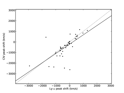
In order to improve the extrapolation of the intrinsic flux, we will need to exploit correlations between the Lyman- emission components and other spectral features (emission lines or continuum luminosity), either through constraints applied to traditional multi-component models, or through the use of principal component analysis. For instance, Shang et al. (2007) cite a correlation between the Lyman- and C iv line shifts. We find a similar correlation in our sample, which we show in Figure 19. The figure demonstrates that the shifts of the lines (determined from fits of a quadratic function to points near the peak) are well correlated (the correlation coefficient is $0.68$, but would be substantially larger with the exclusion of a few outliers). Tytler & Fan (1992), on the other hand, failed to find significant correlations between the shifts of this (and any other) pair of lines when they carefully determined systematic redshifts from multiple emission lines. This suggests that the correlation we see may be due, at least in part, to errors in the determination of the systematic redshift. For our purposes, however, it does not matter why the correlation appears, only that it could be exploited to reduce the uncertainty on the location of the intrinsic Lyman- emission line. In addition, one could possibly use more detailed multi-component fits to the shape of the C iv line as a template for both the Lyman- and N v lines. We expect to be able to reduce the flux errors to the point that they are negligible in comparison to other sources of uncertainty.

Figure 19: Shift of the C iv ($1549$ Å) line peak versus shift of the Lyman- peak. The solid line is the unweighted least-squares fit to the plotted points. The dotted line indicates equal shifts. Note that this plot is preliminary.

In addition to improving the spectral fits, we may be able increase the amount of information extracted from the optical depth profiles. Binning the optical depth values, as we have done in performing our K-S tests, discards most of the wavelength information. Conceivably, there is additional information in the detailed wavelength-dependence of the optical depth profiles, extractable with a different statistical comparison to the model profiles.

Another source of additional information is the Lyman- region of the absorption spectrum. While its interpretation is complicated by the overlying Lyman- absorption, careful analysis and comparison with simulations should allow it to supplement the Lyman- fits (e.g. Mesinger & Haiman, 2004).

Such improvements should be explored in order to take full advantage of future samples of high-$z$ quasars. As surveys push deeper, more $z>6$ quasars are constantly being discovered. For example, the Canada-France High-z Quasar Survey (Willott et al., 2009) found 10 new $z>5.9$ quasars, including 2 at $z>6.2$, the SDSS Deep Stripe (Jiang et al., 2008) yielded 5 new $z>5.85$ quasars, and UKIDSS (Mortlock et al., 2008) found one at $z=6.13$. The quasar luminosity function is extremely steep at the bright end that is currently being sampled at high redshift, meaning that modest increases in the sensitivity of future surveys should yield large increases in the number of discovered quasars. Even if the available spectra of such objects have significantly poorer signal-to-noise ratios than current state-of-the-art $z>6$ quasar spectra, they should still be suitable for this purpose, since density fluctuations dominate the scatter in the current results.

The techniques outlined here could also be applied to a wider range of problems. The models (minus the IGM damping wing) and statistical techniques described here for absorption spectra of $z>6$ quasars can just as well be applied at $z<6$ to probe the density and ionizing background near quasars. As LSST and other future surveys perform deep searches for high-$z$ objects, many lower-redshift quasars will be discovered, which will be valuable as probes of typical quasar environments after the end of reionization. At these lower redshifts, rather than creating a well-defined H ii region, quasars exhibit a “proximity effect” (Bajtlik, Duncan & Ostriker, 1988) on the nearby Lyman- forest, reducing the amount of absorption near the source redshift. Kirkman & Tytler (2008), by studying the transverse and line-of-sight proximity effects of quasars at $z\sim 2$, found intriguing evidence of large-scale overdensities near the quasars, as well as evidence for quasar lifetimes shorter than $10^{6}$ years. Other previous studies (Rollinde et al., 2005; Guimarães et al., 2007; Dall’Aglio, Wisotzki & Worseck, 2008) have also explored the proximity effect at $z<4.5$. All of these groups estimated the underlying continuum by iterative fitting to transmission windows between Lyman- forest lines. This technique is limited to $z\la 4.5$, since beyond this redshift the Lyman- forest is too thick to reliably infer the continuum. Above this redshift, the continuum must be extrapolated from unabsorbed regions of the spectrum. With the improved spectral modeling techniques we hope to develop, a uniform analysis of the proximity effect could be performed from low redshift through $z>6$, without having to change the techniques used to model the underlying spectrum.

8 Acknowledgments

We would like to thank Drs. Jules Halpern, Xiaohui Fan, David Schiminovich, Greg Bryan, and David Helfand for useful discussions as this project evolved. We would also like the thank our reviewer, Dr. Brian Espey, for insightful and constructive feedback.

Data presented in this paper were obtained from the Multimission Archive at the Space Telescope Science Institute (MAST). STScI is operated by the Association of Universities for Research in Astronomy, Inc., under NASA contract NAS5-26555. This research has made use of the NASA/IPAC Extragalactic Database (NED) which is operated by the Jet Propulsion Laboratory, California Institute of Technology, under contract with the National Aeronautics and Space Administration. This work was supported by the Polányi Program of the Hungarian National Office for Research and Technology (NKTH).

Appendix A Aligning and coadding spectra

All GHRS and some FOS (rapid-readout mode) datasets are composed of sets of separate exposures. These separate spectra must be aligned before being coadded to preserve spectral resolution. Also, some objects were observed multiple times with the same instrument configuration, and we wanted to coadd these spectra to maximize the signal-to-noise ratio. We chose to only coadd spectra with the same instrument configuration (instrument, grating, and aperture) so that we would not be combining spectra with different resolutions. Therefore we ended up with multiple spectra for some objects.

Our code automatically tries three different methods for aligning the spectra and chooses the one that minimizes the deviations between the input spectra and the mean (as defined below). The methods are to align the spectra with no offsets, based simply on the supplied wavelength coordinates for each spectrum, to align the spectra by maximizing the correlation function, and to first smooth the spectra, then align them by maximizing the correlation between smoothed spectra. The method that minimizes deviations between the aligned spectra and the mean spectrum (as measured by $s_{\mathrm{RMS}}$, defined below), is chosen for the final output. We exclude $10\%$ of the pixels with the lowest signal-to-noise ratio in the mean spectrum, then sum over all of the remaining pixels in each input spectrum in order to characterize the quality of the alignment:

$$s_{\mathrm{RMS}}\equiv\sqrt{\frac{1}{n}\sum_{i}{\left(\frac{f_{i}-\langle f\rangle_{i}}{E(S_{i})}\right)^{2}}}$$ (21)

where $f_{i}$ is the flux value for a pixel in an input spectrum, $\langle f\rangle_{i}$ is the flux value in the corresponding pixel in the mean spectrum, and $E(S_{i})$ is the expectation value of the standard deviation for that pixel, given by

$$E(S_{i}^{2})=\frac{1}{n}\sum_{j}{\sigma_{j}^{2}}$$ (22)

, where $\sigma_{j}$ is the uncertainty on flux value $j$, and the sum is over all of the input pixels contributing to a single pixel in the mean spectrum.

The general procedure for aligning and coadding spectra is as follows:

Spectra are interpolated onto a common, uniform, wavelength grid, then (if desired) smoothed with a Gaussian kernel ($\sigma=3$ pixels).

Aligning the spectra: One spectrum is chosen as the reference spectrum and the correlation function is calculated between it and each remaining spectrum. The correlation between the reference spectrum $F$ and another spectrum $f$ as a function of pixel offset $s$ is

$$C_{F,f}(s)=\sum_{i}{\left(F_{i}-\langle F\rangle\right)\left(f_{i+s}-\langle f\rangle\right)},$$ (23)

where $F_{i}$ is the flux in pixel $i$ of the reference spectrum, $f_{i+s}$ is the flux in pixel $i+s$ in the other spectrum, and $\langle F\rangle$ and $\langle f\rangle$ are the mean flux values of each spectrum.

For each spectrum, the offset is calculated by finding the peak of a parabola passing through the maximum of the correlation function and its two neighboring points. The wavelength coordinates of the spectra are then shifted by the calculated offset and the spectra are reinterpolated onto a common wavelength scale.

Coadding spectra: Spectra are coadded (flux values for each pixel are averaged), excluding outliers and choosing a weighting scheme that maximizes the signal-to-noise. If the spectra have an average signal-to-noise ratio of less than 2, we use an unweighted mean of the pixel values from each spectrum. Otherwise the weights are $w_{i}=F_{i}/\sigma_{i}^{2}$, where $F_{i}$ is the flux in pixel $i$ and $\sigma_{i}$ is the uncertainty. If the uncertainties are Poisson-dominated, this yields $w_{i}=h\nu d\nu_{i}dt_{i}A_{i}$ where $d\nu$ is the bandwidth of the pixel, $dt$ is the integration time, and $A$ is the effective area. This has the advantage over the traditional $w_{i}=\sigma_{i}^{-2}$ of not biasing the results when the uncertainty is estimated from the data. We also propagate the statistical uncertainties to calculate the uncertainties for each pixel in the weighted mean spectrum.

Excluding low signal-to-noise spectra: If we are using the unweighted mean, then spectra are excluded if their signal-to-noise ratio is below $\{[n^{2}/(n-1)]-(n-1)\}^{-1/2}$ times the mean signal-to-noise ratio. This threshold defines the approximate level below which adding a spectrum actually degrades the overall signal-to-noise ratio.

Normalizing spectra: We compare the normalization of each input spectrum to the mean by calculating the mean fractional flux offset between it and the weighted mean spectrum. The significance of the flux offset is then calculated, and any spectra that are more than $3\sigma$ below the mean are normalized to have the same average flux as the mean. We only re-normalize spectra below the mean because we assume that flux offsets are caused by non-optimal positioning of the source in the aperture, which can only result in missing flux. This procedure is iterated until all mean flux differences are less than $3\sigma$. Any bias introduced by this procedure should be unimportant, since we only care about the overall shape of the spectrum, not its normalization.

Outlier exclusion proceeds in two phases. First we iteratively exclude individual pixels indentified as outliers, then we exclude all data at wavelength coordinates where the spectrum-to-spectrum dispersion is too high.

Excluding outlying pixel values: We calculate the difference between each pixel value in the input spectra and the value of that pixel in the mean spectrum, and calculated the uncertainty of that difference. We also calculate the standard deviation of the values for each pixel. Any value deviating more than 5 times the propagated uncertainty from the mean and more than 1 standard deviation from the mean is excluded.

Flagging bad pixels: The expected level of deviation $S$ among the $n$ data points for each pixel is given by $E(S^{2})=(1/n)\sum{\sigma_{i}^{2}}$, where $\sigma_{i}$ are the uncertainties on each value. any pixel in which the standard deviation of the input values is higher than the $3S$ is flagged as bad and excluded from future analysis.

Finally an output spectrum is constructed by averaging the input spectra, with wavelength offsets and weights if appropriate, and excluding any detected outliers.

Appendix B Automatic absorption feature detection

In order to characterize the intrinsic quasar spectra, we need to exclude absorption features from our fits, and we need to do so automatically to take advantage of large samples of quasars and have reproducible results. At the same time, we want to avoid biasing our fits by removing low-flux pixels that represent real variations in the intrinsic quasar spectrum. We do this using two rounds of iterative feature detection. In the first round, we apply our absorption-feature threshold only to pixels deviating below the model spectrum. In the second round we apply the same threshold to pixels deviating above the model spectrum. This way, if our threshold is too stringent we will notice spurious flagging of positive deviations. This had the unexpected benefit of automatically detecting and excluding pixels influenced by blending with neighboring broad emission lines in several cases.

Our feature detection is iterative. First, we fit a model to the observed flux profile. We then smooth the observed spectrum, model spectrum, and the error spectra of each, and calculate the difference between the smoothed model and observed spectra. We then calculate a feature detection threshold

$$f_{\mathrm{thresh}}^{2}(\lambda)=[c_{f}~{}f_{\mathrm{fit}}(\lambda)]^{2}+[c_{e}~{}\sigma_{\mathrm{obs}}(\lambda)]^{2}+\sigma_{\mathrm{fit}}^{2}(\lambda)$$ (24)

using statistical uncertainties on the model flux ($\sigma_{\mathrm{fit}}$), uncertainty on the measured flux ($\sigma_{\mathrm{obs}}$), and the observed flux ($f_{\mathrm{fit}}$). The constants $c_{f}=0.05$, $c_{e}=6$, were chosen by hand to be rather conservative. That is, we err on the side of not excluding features, rather than risk falsely excluding “good” pixels. Any pixel in which the magnitude of the smoothed residuals exceeds the threshold is flagged as an absorption or emission feature. Pixel within $\pm\Delta\lambda$ of a flagged pixel are then excluded around the detected features, and the fit is repeated, excluding the flagged features (or only the flagged absorption features in the first round).

$$\Delta\lambda=2\sqrt{w_{\mathrm{min}}^{2}+w_{\mathrm{Inst}}^{2}},$$ (25)

where $w_{\mathrm{min}}=0.75$ Å and $w_{\mathrm{Inst}}=\mathrm{FWHM}/2.355$, with $\mathrm{FWHM}$ being the full width at half maximum of the instrumental line spread function (LSF). The iteration stops once no more features are flagged.

References

- Bajtlik et al. (1988) Bajtlik S., Duncan R. C., Ostriker J. P., 1988, ApJ, 327, 570
- Baldwin (1977) Baldwin J. A., 1977, ApJ, 214, 679
- Barkana & Loeb (2003) Barkana R., Loeb A., 2003, Nature, 421, 341
- Barkana & Loeb (2004) Barkana R., Loeb A., 2004, ApJ, 601, 64
- Becker et al. (2001) Becker R. H., et al., 2001, AJ, 122, 2850
- Bolton & Haehnelt (2007) Bolton J. S., Haehnelt M. G., 2007, MNRAS, 381, L35
- Boroson (2005) Boroson T., 2005, AJ, 130, 381
- Cen & Haiman (2000) Cen R., Haiman Z., 2000, ApJL, 542, L75
- Dall’Aglio et al. (2008) Dall’Aglio A., Wisotzki L., Worseck G., 2008, A&A, accepted, preprint arXiv:0801.1767
- Decarli et al. (2008) Decarli R., Labita M., Treves A., Falomo R., 2008, MNRAS, 387, 1237
- Dietrich et al. (2002) Dietrich M., Hamann F., Shields J. C., Constantin A., Vestergaard M., Chaffee F., Foltz C. B., Junkkarinen V. T., 2002, ApJ, 581, 912
- Espey & Andreadis (1999) Espey B., Andreadis S., 1999, in Ferland G., Baldwin J., eds, Quasars and Cosmology Vol. 162 of Astronomical Society of the Pacific Conference Series, Observational Evidence for an Ionization-Dependent Baldwin Effect. pp 351–+
- Fan et al. (2006) Fan X., Carilli C. L., Keating B., 2006, ARA&A, 44, 415
- Fan et al. (2006) Fan X., et al., 2006, AJ, 131, 1203
- Fan et al. (2006) Fan X., Strauss M. A., Becker R. H., White R. L., Gunn J. E., Knapp G. R., Richards G. T., Schneider D. P., Brinkmann J., Fukugita M., 2006, AJ, 132, 117
- Gnedin (2000) Gnedin N. Y., 2000, ApJ, 542, 535
- Guimarães et al. (2007) Guimarães R., Petitjean P., Rollinde E., de Carvalho R. R., Djorgovski S. G., Srianand R., Aghaee A., Castro S., 2007, MNRAS, 377, 657
- Gunn & Peterson (1965) Gunn J. E., Peterson B. A., 1965, ApJ, 142, 1633
- Hogg (1999) Hogg D. W., 1999, preprint, arXiv:astro-ph/9905116
- Jiang et al. (2008) Jiang L., Fan X., Annis J., Becker R. H., White R. L., Chiu K., Lin H., Lupton R. H., Richards G. T., Strauss M. A., Jester S., Schneider D. P., 2008, AJ, 135, 1057
- Kirkman & Tytler (2008) Kirkman D., Tytler D., 2008, MNRAS, 391, 1457
- Komatsu et al. (2008) Komatsu E., Dunkley J., Nolta M. R., Bennett C. L., Gold B., Hinshaw G., Jarosik N., Larson D., Limon M., Page L., Spergel D. N., Halpern M., Hill R. S., Kogut A., Meyer S. S., Tucker G. S., Weiland J. L., Wollack E., Wright E. L., 2008, preprint, arXiv:0803.0547
- Kramer & Haiman (2008) Kramer R. H., Haiman Z., 2008, MNRAS, 385, 1561
- Lidz et al. (2007) Lidz A., McQuinn M., Zaldarriaga M., Hernquist L., Dutta S., 2007, ApJ, 670, 39
- Madau & Rees (2000) Madau P., Rees M. J., 2000, ApJL, 542, L69
- Marziani et al. (2008) Marziani P., Sulentic J. W., Dultzin D., 2008, in Revista Mexicana de Astronomia y Astrofisica Conference Series Vol. 32 of Revista Mexicana de Astronomia y Astrofisica Conference Series, The Broad Line Region of Quasars. pp 69–73
- Maselli et al. (2007) Maselli A., Gallerani S., Ferrara A., Choudhury T. R., 2007, MNRAS, 376, L34
- McIntosh et al. (1999) McIntosh D. H., Rix H.-W., Rieke M. J., Foltz C. B., 1999, ApJL, 517, L73
- McQuinn et al. (2008) McQuinn M., Lidz A., Zaldarriaga M., Hernquist L., Dutta S., 2008, MNRAS, 388, 1101
- Mesinger & Furlanetto (2008) Mesinger A., Furlanetto S. R., 2008, MNRAS, 385, 1348
- Mesinger & Haiman (2004) Mesinger A., Haiman Z., 2004, ApJL, 611, L69
- Mesinger & Haiman (2007) Mesinger A., Haiman Z., 2007, ApJ, 660, 923
- Miralda-Escudé (1998) Miralda-Escudé J., 1998, ApJ, 501, 15
- Miralda-Escudé et al. (2000) Miralda-Escudé J., Haehnelt M., Rees M. J., 2000, ApJ, 530, 1
- Mortlock et al. (2008) Mortlock D. J., Patel M., Warren S. J., Venemans B. P., McMahon R. G., Hewett P. C., Simpson C., Sharp R. G., Burningham B., Ellis S., Gonzales-Solares E. A., Huelamo N., 2008, preprint, arXiv:0810.4180
- Popović et al. (2004) Popović L. Č., Mediavilla E., Bon E., Ilić D., 2004, A&A, 423, 909
- Richards et al. (2002) Richards G. T., Vanden Berk D. E., Reichard T. A., Hall P. B., Schneider D. P., SubbaRao M., Thakar A. R., York D. G., 2002, AJ, 124, 1
- Rollinde et al. (2005) Rollinde E., Srianand R., Theuns T., Petitjean P., Chand H., 2005, MNRAS, 361, 1015
- Shang et al. (2007) Shang Z., Wills B. J., Wills D., Brotherton M. S., 2007, AJ, 134, 294
- Shields (2007) Shields J. C., 2007, in Ho L. C., Wang J.-W., eds, The Central Engine of Active Galactic Nuclei Vol. 373 of Astronomical Society of the Pacific Conference Series, Emission-Line versus Continuum Correlations in Active Galactic Nuclei. p. 355
- Thomas & Zaroubi (2008) Thomas R. M., Zaroubi S., 2008, MNRAS, 384, 1080
- Tytler & Fan (1992) Tytler D., Fan X.-M., 1992, ApJS, 79, 1
- Vanden Berk et al. (2001) Vanden Berk D. E., et al., 2001, AJ, 122, 549
- Verner et al. (1994) Verner D. A., Barthel P. D., Tytler D., 1994, A&AS, 108, 287
- Willott et al. (2009) Willott C. J., Delorme P., Reyle C., Albert L., Bergeron J., Crampton D., Delfosse X., Forveille T., Hutchings J. B., McLure R. J., Omont A., Schade D., 2009, prerint, arXiv 0901.0565
- Wyithe & Loeb (2004) Wyithe J. S. B., Loeb A., 2004, Nature, 427, 815
- Zamanov et al. (2002) Zamanov R., Marziani P., Sulentic J. W., Calvani M., Dultzin-Hacyan D., Bachev R., 2002, ApJL, 576, L9