Noether symmetry approach in phantom quintessence cosmology

Abstract

In the framework of phantom quintessence cosmology, we use the Noether Symmetry Approach to obtain general exact solutions for the cosmological equations. This result is achieved by the quintessential (phantom) potential determined by the existence of the symmetry itself. A comparison between the theoretical model and observations is worked out. In particular, we use type Ia supernovae and large scale structure parameters determined from the 2-degree Field Galaxy Redshift Survey (2dFGRS)and from the Wide part of the VIMOS-VLT Deep Survey (VVDS). It turns out that the model is compatible with the presently available observational data. Moreover we extend the approach to include radiation. We show that it is compatible with data derived from recombination and it seems that quintessence do not affect nucleosynthesis results.

I Introduction

Recent analysis of the three year WMAP data w ; m ; p provides no indication of any significant deviations from Gaussianity and adiabaticity of the CMBR power spectrum and therefore suggests that the Universe is spatially flat to within the limits of observational accuracy. Further, the combined analysis of the three-year WMAP data with the Supernova Legacy Survey (SNLS), in w , constrains the equation of state $w_{de}$, corresponding to almost ${74\%}$ of dark energy present in the currently accelerating Universe, to be very close to that of the cosmological constant value. The marginalized best fit values of the equation of state parameter gave $-1.14\leq w_{de}\leq-0.93$ at $68\%$ confidence level. Thus, it was realized that a viable cosmological model should admit a dynamical equation of state that might have crossed the phantom value $w=-1$, in the recent epoch of cosmological evolution. Phantom fluid was first investigated in the current cosmological context by Caldwell caldwell99 , who also suggested the name referring to the fact that phantom (or ghost) must possess negative energy which leads to instabilities on both classical and quantum level instabilities ; nojiri04 . Since it violates the energy conditions, it also could put in doubt the pillars of general relativity and cosmology such as: the positive mass theorems, the laws of black hole thermodynamics, the cosmic censorship, and causality he ; visser . On the other hand, phantom becomes a real challenge for the theory, if its support from the supernovae Ia-Type (SNeIa) data is really so firm. From the theoretical point of view, a release of the assumption of an analytic equation of state which relates energy density and pressure and does not lead to energy conditions violation (except for the dominant one) may also be useful barrow04 . As for the explanation of the SNeIa data, phantom is also useful in killing the doubled positive pressure contribution in several braneworld models braneIa .

Phantom type of matter was also implicitly suggested in cosmological models with a particle production john88 , in higher-order theories of gravity models Pollock88 , Brans-Dicke models, in non-minimally coupled scalar field theories starob00 ; mareknmc1 , in "mirage cosmology" of the braneworld scenario kiritsis , and in kinematically-driven quintessence (k-essence) models chiba ; sanyal , for example. Such phantom models have well-known problems but, nevertheless, have also been widely studied as potential dark energy candidates, and actually the interest in phantom fields has grown vastly during the last years and various aspects of phantom models have been investigated Frampt02 ; Frampt03 ; trodden1 ; trodden2 ; Bastero01 ; Bastero02 ; abdalla04 ; Erickson ; LiHao03 ; singh03 ; nojiri031 ; nojiri032 ; nojiri033 ; nojiri034 ; simphan ; onemli ; diaz ; saridakis1 .

One of the most interesting features of phantom models is that they allow for a Big-Rip (BR) curvature singularity, which appears as a result of having the infinite values of the scale factor $a(t)\to\infty$ at a finite future. However, as it was already mentioned, the evidence for phantom from observations is mainly based on the assumption of the barotropic equation of state which tightly constraints the energy density and the pressure. It is puzzling barrow04 that for Friedmann cosmological models, which do not admit an equation of state which links the energy density $\varrho$ and the pressure $p$, a sudden future singularity of pressure may appear. This is a singularity of pressure only, with finite energy density which has an interesting analogy with singularities which appear in some inhomogeneous models of the Universe dabrowski95 ; inhosfs .

Recently, phantom cosmologies which lead to a quadratic polynomial in canonical Friedmann equation have been investigated phantom1 , showing that interesting dualities exist between phantom and ordinary matter models which are similar to dualities in superstring cosmologies meissner91 ; superjim . These dualities were generalized to non-flat and scalar field models lazkoz1 ; lazkoz2 ; lazkoz3 ; lazkoz4 ; lazkoz5 ; lazkoz6 ; lazkoz7 ; lazkoz8 ; lazkoz9 ; lazkoz10 ; lazkoz11 ; lazkoz12 ; lazkoz13 , brane models calcagni , and are also related to ekpyrotic models ekpyrotic ; triality . Furthermore, some theoretical studies have been devoted to shed light on phantom dark energy within the quantum gravity framework, since, despite the lack of such a theory at present, we can still make some attempts to probe the nature of dark energy according to some of its basic principles saridakis2 .

Finally, phantom cosmology can provides the opportunity to "connect" the phantom driven (low energy $meV$ scale) dark energy phase to the (high energy GUT scale) inflationary era. This is possible because the energy density increases in phantom cosmology. Concrete models in this sense have been recently elaborated with some interesting results biswas .

In this paper, we want to investigate if the existence of phantom fields can be connected to Noether symmetries. Such an issue becomes recently extremely important due to the fact that several phenomenological models have been constructed but, some of them, have no self-consistent theoretical foundation. The idea to derive the equation of state from symmetries is not new heller and recently has been applied to dark energy szydlowski . From a mathematical point of view, the general consideration is that symmetries greatly aid in finding exact solutions heller ; cimento . Besides, due to the Noether theorem, symmetries are always related to conserved quantities which, in any case, can be considered as conserved "charges". Specifically, the form of the self-interacting scalar-field potential is "selected" by the existence of a symmetry and then the dynamics can be controlled. The equation of state, being related to the form of scalar-field potential, is determined as well. However, the symmetry criterion is not the only that can be invoked to discriminate physically consistent models but it could be considered a very straightforward one since, as we will see below, it allows also to achieve exact solutions.

In Sect.II, we actually show that phantom fields come out by requiring the existence of Noether symmetry to the Lagrangian describing a standard single scalar field quintessential cosmological model: we show that it allows a phantom dark energy field, and also provides an explicit form for the (phantom) self-interaction potential. Sect. III studies how this gives rise to exact and general solutions. Also extending the approach to include radiation, we show that it is also compatible with the post recombination observational data and that quintessence does not influence the results of nucleosynthesis. In Sect IV, we work out a comparison between the theoretical solution and observational dataset, as the publicly available data on SNeIa, the parameters of large scale structure determined from the 2-degree Field Galaxy Redshift Survey (2dFGRS)and from the Wide part of the VIMOS-VLT Deep Survey (VVDS). In Sect.V, we discuss the presented results and draw conclusions.

II The Noether Symmetry Approach

The Noether Symmetry Approach has revealed a useful tool in order to find out exact solutions, in particular in cosmology cimento ; cqgarturo ; defelice ; leandros . The existence of the Noether symmetry allows to reduce the dynamical system that, in most of cases, results integrable. It is interesting to note that the self-interacting potentials of the scalar field leandros , the couplings cimento or the overall theory defelice , if related to a symmetry (i.e. a conserved quantity) have a physical meaning. In this sense, the Noether Symmetry Approach is also a physical criterion to select reliable models (see defelice for a discussion).

In the present case, let us consider a matter–dominated model in homogeneous and isotropic cosmology with signature $(-,+,+,+)$ for the metric, with a single scalar field, $\phi$, minimally coupled to the gravity. It turns out that the point-like Lagrangian action takes the form

$${\cal L}=3a\dot{a}^{2}-a^{3}\left(\epsilon\frac{\dot{\phi}^{2}}{2}-V(\phi)\right)+Da^{-3(\gamma-1)}\,$$ (1)

where $a$ is the scale factor and the constant $D$ is a constant defined in such a way that the matter density $\rho_{m}$ is expressed as $\rho_{m}=D(a_{o}/a)^{3\gamma}$, where $1\leq\gamma\leq 2$. For the moment, we will limit our analysis to $\gamma=1$, corresponding to cosmological dust. The value of the constant $\epsilon$ discriminates between standard and phantom quintessence fields: in the former case, it is $\epsilon=1$; in the latter, it is $\epsilon=-1$. The effective pressure and energy density of the $\phi$-field are given by

$$p_{\phi}=\epsilon\frac{1}{2}\dot{\phi}^{2}-V(\phi)\,,$$ (2)

$$\rho_{\phi}=\epsilon\frac{1}{2}\dot{\phi}^{2}+V(\phi)\,.$$ (3)

These two expressions define an effective equation of state $w_{\phi}=\displaystyle\frac{p_{\phi}}{\rho_{\phi}}$, which drives the behavior of the model. The field equations are

$$2\frac{\ddot{a}}{a}+H^{2}+\epsilon\frac{1}{2}\dot{\phi}^{2}-V(\phi)=0,$$ (4)

$$\frac{\ddot{a}}{a}+3H\dot{\phi}+\epsilon V^{\prime}(\phi)=0,$$ (5)

$$3H^{2}=\rho_{\phi}+\rho_{m},$$ (6)

where prime denotes derivative with respect to $\phi$, while dot denotes derivative with respect to time.

The Noether theorem states that, if there exists a vector field $X$, for which the Lie derivative of a given Lagrangian $L$ vanishes i.e. $L_{X}{\cal L}=0$, the Lagrangian admits a Noether symmetry and thus yields a conserved current cimento . In the Lagrangian under consideration, the configuration space is ${\cal M}=\{a,\phi\}$ and the corresponding tangent space is $T{\cal M}=\{a,\phi,\dot{a},\dot{\phi}\}$. Hence the infinitesimal generator of the Noether symmetry is

$$X=\alpha\frac{\partial}{\partial{a}}+\beta\frac{\partial}{\partial{\phi}}+\dot{\alpha}\frac{\partial}{\partial{\dot{a}}}+\dot{\beta}\frac{\partial}{\partial{\dot{\phi}}},$$ (7)

where $\alpha$ and $\beta$ are both functions of $a$ and $\phi$ and

$$\dot{\alpha}\equiv\frac{\partial\alpha}{\partial a}\dot{a}+\frac{\partial\alpha}{\partial\phi}\dot{\phi}$$ (8)

$$\dot{\beta}\equiv\frac{\partial\beta}{\partial a}\dot{a}+\frac{\partial\beta}{\partial\phi}\dot{\phi}.$$ (9)

The Cartan one–form is

$$\theta_{\cal L}=\frac{\partial{\cal L}}{\partial{\dot{a}}}da+\frac{\partial{\cal L}}{\partial{\dot{\phi}}}d\phi.$$ (10)

The constant of motion $Q=i_{X}\theta_{\cal L}$ is given by

$$Q=\alpha(a,\phi)\frac{\partial{\cal L}}{\partial{\dot{a}}}+\beta(a,\phi)\frac{\partial{\cal L}}{\partial{\dot{\phi}}}.$$ (11)

If we demand the existence of a Noether symmetry, $L_{X}{\cal L}=0$, we get the following equations,

$$\alpha+2a\frac{\partial{\alpha}}{\partial{a}}=0$$ (12)

$$6\frac{\partial{\alpha}}{\partial{\phi}}-\epsilon a^{2}\frac{\partial{\beta}}{\partial{a}}=0$$ (13)

$$3\alpha+2\epsilon a\frac{\partial{\beta}}{\partial{\phi}}=0$$ (14)

$$3V(\phi)\alpha+aV^{{}^{\prime}}(\phi)a\beta=0$$ (15)

We have now to look for conditions on the integrability of this set of equations, limiting ourselves to the phantom case (1.e., $\epsilon=-1$), since the standard case has been already investigated in rubscud ; marek1 . It is possible to assume that $\alpha$ and $\beta$ are separable (and non–null), i.e.

$$\alpha(a,\phi)=A_{1}(a)B_{1}(\phi),\leavevmode\nobreak\ \leavevmode\nobreak\ \leavevmode\nobreak\ \beta(a,\phi)=A_{2}(a)B_{2}(\phi).$$ (16)

This is not true in general but, in such a case, it is straightforward to achieve a solution for the system (12-15). It is

$$\alpha=\frac{2A\cos\left(\frac{1}{2}\sqrt{\frac{3}{2}}\phi\right)}{\sqrt{a}}\,,$$ (17)

$$\beta=\frac{-2\sqrt{6}A\sin\left(\frac{1}{2}\sqrt{\frac{3}{2}}\phi\right)}{a\sqrt{a}}\,,$$ (18)

$$V(\phi)=V_{0}\sin\left(\frac{1}{2}\sqrt{\frac{3}{2}}\phi\right)^{2}$$ (19)

which selects the Noether symmetry.

III Solutions from new coordinates and Lagrangian

Once that $X$ is found, it is then possible to find a change of variables $\{a,\phi\}\rightarrow\{u,v\}$, such that one of them (say $u$, for example) is cyclic for the Lagrangian ${\cal L}$ in Eq. (1), and the transformed Lagrangian produces a reduced dynamical system which is generally solvable. Solving the system of equations $i_{X}du=1$ and $i_{X}dv=0$ (where $i_{X}du$ and $i_{X}dv$ are the contractions between the vector field $X$ and the differential forms $du$ and $dv$, respectively), we obtain:

$$a=(v+9A^{2}u^{2})^{\frac{1}{3}}$$ (20)

$$\phi=2\sqrt{2/3}\arccos{\frac{(3Au)}{\sqrt{v+9A^{2}u^{2}}}}.$$ (21)

Under this transformation, the Lagrangian takes the suitable form

$${\cal L}=D+vV_{0}+\frac{\dot{v}^{2}}{3v}+12A^{2}\dot{u}^{2}\,,$$ (22)

where $u$ is the cyclic variable. The conserved current gives

$$Q=\frac{\partial{\cal L}}{\partial\dot{u}}=24A^{2}\dot{u}=B,$$ (23)

which can be trivially integrated to obtain $u(t)=Bt+C$. We use now the energy condition $E_{\cal L}=0$ to find $v$. We obtain the following differential equation

$$\dot{v(t)}^{2}-3v(t)\left(D+V_{0}v(t)-12A^{2}\dot{u(t)}^{2}\right)=0\,.$$ (24)

It is a first order equation which for , i.e. can be factorized into the form

$$\left(p-F_{1}\right)\left(p-F_{2}\right)=0,$$ (25)

being $p=\dot{v(t)}$ and $F_{i}=F_{i}(t,v)$. We are then left with solving two first-degree equations $p=F_{i}(t,v)$. Writing the solutions to these first-degree equations as $G_{i}(t,v)=0$ the general solution to Eq. (24) is given by the product $G_{1}(t,v)G_{2}(t,v)=0$. It turns out that:

$$v(t)=\frac{\exp{(-\sqrt{3V_{0}}t)}}{16V_{0}^{2}}\left(\exp{(\sqrt{3V_{0}}t)}+48A^{2}B^{2}V_{0}-4DV_{0}\right)^{2}.$$ (26)

The substitution of the functions $a=a(u,v)$ and $\phi=\phi(u,v)$ into Eqs. (20,21) yields

$$a(t) = \left(9\omega^{2}t^{2}+\frac{\left(\exp{-\sqrt{3V_{0}}t}\right)\left(\exp{\sqrt{3V_{0}}t}+48\omega^{2}V_{0}-4DV_{0}\right)^{2}}{16V_{0}^{2}}\right)^{\frac{1}{3}}$$ (27)

$$\phi(t) = 2\sqrt{\frac{2}{3}}\arccos{\left(\frac{3ABt}{\sqrt{9\omega^{2}t^{2}+\frac{\left(\exp{-\sqrt{3V_{0}}t}\right)\left(\exp{\sqrt{3V_{0}}t}+48\omega^{2}V_{0}-4DV_{0}\right)^{2}}{16V0^{2}}}}\right)},$$ (28)

where we have defined $\omega=AB$. Setting $a(0)=0$, we can construct a relation among the integration constants $\omega$, $D$ and $V_{0}$: actually it turns out that $D=\frac{1+48\omega^{2}V_{0}}{4V0}$. To determine the integration constant $\omega$, we set the present time $t_{0}=1$. This fixes the time-scale according to the (formally unknown) age of the Universe. That is to say that we are using the age of the Universe, $t_{0}$, as a unit of time. We then set $a_{0}=a(1)=1$, to obtain

$$\omega=\frac{\sqrt{8+\frac{1}{V_{0}^{2}}-\cosh{\sqrt{3V_{0}}}}}{V_{0}^{2}}.$$ (29)

The two conditions specified above allow one to express all the basic cosmological parameters in terms of $V_{0}$, the constant that determines the scale of the potential. It is not directly measurable. However we can also strongly constrain its range of variability through its relation with the Hubble constant: actually because of our choice of time unit, the expansion rate $H(t)$ is dimensionless, so that our Hubble constant $\widehat{H}_{0}=H(t_{0})$ is clearly of order 1 and not (numerically) the same as the $H_{0}$ that is usually measured in ${\rm kms^{-1}Mpc^{-1}}$. Actually, we can consider the relation

$$h=9.9\frac{{\widehat{H}_{0}}}{\tau}\,,$$ (30)

where, as usual, $h=H_{0}/100$ and $\tau$ is the age of the Universe in $Gy$. We see that $\widehat{H}_{0}$ fixes only the product $h\tau$. In particular, following e.g. w , we can assume that $\tau=13.73^{+0.16}_{-0.15}$, thus we get $h<0.76$ for $\widehat{H}_{0}\approx 1$. Since, according to our parameterization, $\widehat{H}_{0}=\frac{2+16V_{0}^{2}-2\cosh{\sqrt{3V_{0}}}+\sqrt{3V_{0}}\sinh{\sqrt{3V_{0}}}}{24V_{0}^{2}}$, it is possible to constrain the range of variability for $V_{0}$, starting from $\widehat{H}_{0}$. By means of these choices, the exact solutions in Eqs. (27) and (28) can be used to construct all the relevant cosmological parameters. In particular

$$\rho_{\phi} = -\frac{1}{2}\dot{\phi(t)}^{2}+V(\phi)\,,$$ (31)

$$p_{\phi} = -\frac{1}{2}\dot{\phi(t)}^{2}-V(\phi)\,,$$ (32)

$$w_{\phi} = \frac{-\frac{1}{2}\dot{\phi(t)}^{2}+V(\phi)}{-\frac{1}{2}\dot{\phi(t)}^{2}+V(\phi)}\,,$$ (33)

$$\Omega_{\phi} = \frac{\rho_{\phi}}{3H^{2}}\,.$$ (34)

Figure 1: Redshift dependence of the acceleration $\ddot{a}(t)$: the model allows an accelerated phase of expansion, as indicated by the observations.

Figure 2: Redshift dependence of the equation of state parameter $w_{\phi}$ for the some values of $H_{0}$.

Figure 3: Redshift dependence of the equation of state $w_{\phi}$ and the function $\delta(\rho_{\phi}+p_{\phi})=\frac{\rho_{\phi}+p_{\phi}}{\rho_{\phi}}$, which allows to compare the violation of the energy condition with the super-quintessential expansion.

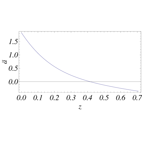
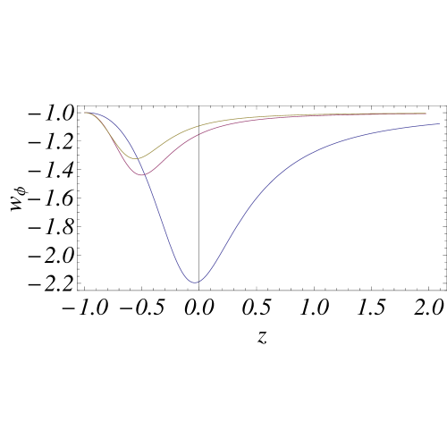
As it is shown in Fig. (1), the model allows an accelerated expansion as indicated from the observations, and being a phantom field exhibits a super-quintessential equations of state, with $w_{\phi}<-1$ (see Fig. (2)), a violation of the weak energy condition (see Fig. (3)). Finally, to conclude this Section, we present the traditional plot $\log{\rho_{\phi}}$ - $\log a$ compared with the matter density (see Fig. (4)). We see that $\rho_{\phi}$ undergoes a transition from a subdominant phase, during the matter dominated era, to a dominant phase. The nowadays accelerated expansion of the Universe can be associated to such a transition. Interestingly, both the subdominant and the dominant phases are characterized by a constant density behavior.

Figure 4: Plot of $\log_{10}{\rho_{\phi}}$ versus ${\log}_{10}a$ (thick line). The dashed lines indicate the log-log plot of $\log_{10}{\rho_{m}}\propto\log_{10}{a^{-3}}$.

Figure 5: Behavior of density parameters of (phantom) quintessence and matter. The fixed point regime, characterized by quintessence density parameter equal to unity ($\Omega_{\phi}=1$), has not yet been reached today, which can be considered a transition epoch.

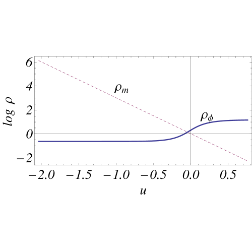
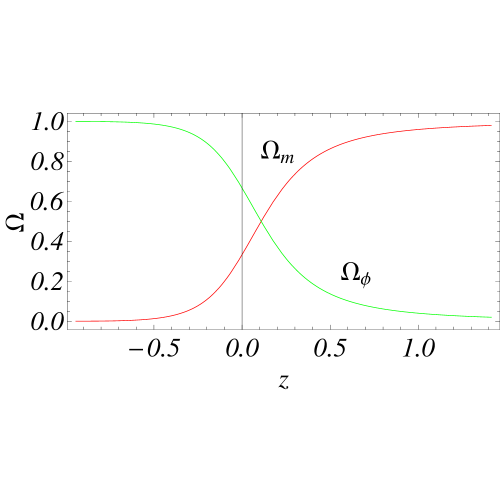
Fig.(5) shows the density parameters of (phantom) quintessence and matter. The fixed point regime, characterized by quintessence density parameter equal to unity ($\Omega_{\phi}=1$), has not yet been reached today. This means that we are living in a transition epoch with $\Omega_{\phi_{0}}\sim 0.7$.

III.1 Including radiation

A more realistic model can be considered by including also radiation beside dust matter and scalar field. In this case, the dynamical equations, as far as we know, do not have analytical solutions and it is not possible to analytically reconstruct the Noether symmetry. Due to these facts, we will relay on numerical solutions.

Let us introduce the new independent variable $u=\log(1+z)=-\log({a(t)/a_{0}})$, where $a_{0}$ is the present value of the scale factor. The Einstein scalar field equations can be written in the form

$$H^{2}=\frac{\rho_{m}+\rho_{r}+V}{3+\frac{1}{2}{\phi}^{\prime 2}}\,,$$ (35)

$$H^{2}\phi^{{}^{\prime\prime}}=\left[-\frac{1}{2}(\rho_{r}+\rho_{m})+V\right]\phi^{\prime}+{\frac{dV}{d\phi}}\,$$ (36)

where $\rho_{r}\sim a^{-4}$ is the energy density of radiation. We numerically solved this system of coupled equations, specifying the initial conditions. The results of numerical integration are shown in Figs.6, 7, and 8.

Figure 6: The Hubble parameter as a function of $u$ in the Universe filled in with matter, radiation and scalar field.

Figure 7: Omega parameters as a function of $u$ in the Universe filled in with matter, radiation and scalar field. $\Omega_{\varphi}$ is marked in green, $\Omega_{r}$ in red and $\Omega_{m}$ in blue.

Figure 8: Plot of $\log_{10}{\rho_{\phi}}$ versus ${\log}_{10}a$ (thick line). The lines indicate the log-log plot of $\log_{10}{\rho_{m}}\propto\log_{10}{a^{-3}}$ and the log-log plot of $\log_{10}(\rho_{r})\propto\log_{10}(a^{-4})$.

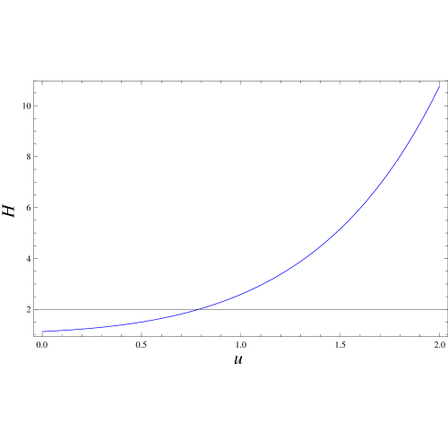
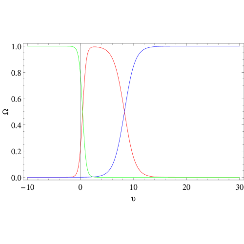
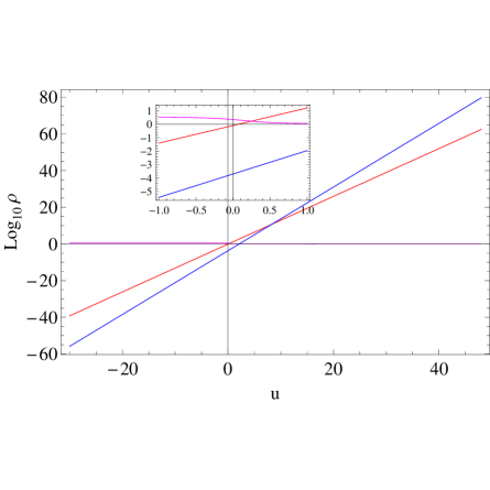
The presence of radiation is hardly changing the behavior of the scalar field, its potential, the Hubble constant and the $w$ parameter of the dark energy equation of state. As expected, the evolution of the $\Omega$ parameters is different. At the initial time (fixed for numerical calculations at $u=30$), radiation dominates the expansion rate of the Universe, with dark energy and matter being sub–dominant. At a redshift of about 5000, the energy density of matter and radiation become comparable and, during a relatively short period, the Universe becomes matter dominated. At a redshift of about $1$ dark energy starts to dominate the expansion rate of the Universe. As result (see, Fig. 10), it follows that during the epoch of nucleosynthesis ($z\sim 10^{9}$) the energy density of the scalar field is much smaller than the energy density of radiation. In particular, during such an epoch, the kinetic terms in the energy density of scalar field vanishes, and the potential terms is constant: in this case, the dark–energy term acts as an effective cosmological constant $\Lambda$, and it does not influence the process of primordial nucleosynthesis.

IV Observational data and predictions

The above phantom scalar field model of quintessence, provides an accelerated expansion of the Universe which could agree, in principle, to the other cosmological behaviors. To test the viability of the model, let us compare now its predictions with some available observational dataset. We concentrate mainly on different kinds of observational data: the publicly available data on SNeIa, the parameters of large scale structure determined starting from the 2-degree Field Galaxy Redshift Survey (2dFGRS)and from the Wide part of the VIMOS-VLT Deep Survey (VVDS).

IV.1 Constraints from SNeIa observations

The model can be constrained by SNeIa dataset presently available. As a starting point, let us take into account the sample of 182 SNIa compiled in Riess07 , which includes the 21 new SNeIa recently discovered by the Hubble Space Telescope (HST), and combines previous SNeIa dataset, namely the Gold Sample compiled in Riess04 , supplemented by the SNLS dataset SNLS .

Figure 9: Observational data from the SNeIa sample fitted against the model. The solid curve is the best fit curve, and the best fits values are $V_{0}=14^{+2}_{-1}$, which corresponds to $\widehat{H}_{0}=0.98^{+0.05}_{-0.04}$ and $\Omega_{\phi}=0.68^{+0.06}_{-0.04}$.

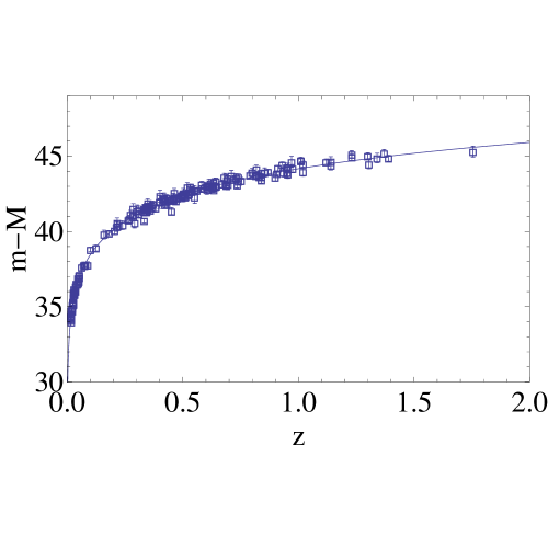
Following a standard procedure, we perform a $\chi^{2}$ analysis comparing the redshift dependence of the theoretical values to the observational estimates of the distance modulus, $\mu=m-M$, which takes the form

$$m-M=5\log{D_{L}(z)}+25.$$ (37)

Moreover, the luminosity distance for a general flat and homogeneous cosmological model can be expressed as an integral of the Hubble function as

$$D_{L}(z) = \frac{c}{H_{0}}(1+z)\int^{z}_{0}\frac{1}{E(\zeta)}d\zeta,$$ (38)

where $E(z)=\frac{H(z)}{H_{0}}$ is related to the Hubble function expressed in terms of $z=a_{0}/a(t)-1$. Let us note that the luminosity distance also depends on the Hubble distance $c/H_{0}$ (which does not depend on the choice of the unit of time). Such freedom allows us to fit $h$ or the a priori unknown age of the Universe $\tau$ using the SNeIa dataset. We find that $\chi_{red}^{2}=1.04$ for 182 data points, and the best fit values are $V_{0}=14^{+3}_{-1}$, which corresponds to $\widehat{H}_{0}=0.98^{+0.05}_{-0.04}$ and $\Omega_{\phi}=0.68^{+0.06}_{-0.04}$. We also get $h=0.72\pm 0.04$. In Fig (9), we compare the best-fit curve with the observational dataset.

IV.2 Dimensionless coordinate distance test

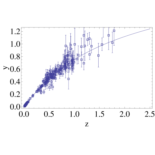
After having explored the Hubble diagram of SNeIa, that is the plot of the distance modulus as a function of the redshift $z$, we want here to follow a very similar, but more general approach, considering as a cosmological observable the dimensionless coordinate distance defined as :

$$y(z)=\int_{0}^{z}{\frac{1}{H(\zeta)}d\zeta}\ .$$ (39)

The variable $y(z)$ does not depend explicitly on $h$ so that any choice of $h$ does not alter the main result. Daly & Djorgovki DD04 have compiled a sample comprising data on $y(z)$ for the 157 SNeIa in the Riess et al. Riess04 Gold dataset and 20 radiogalaxies from RGdata , summarized in Tables 1 and 2 of DD04 . In DD06 , they have added the latest SNeIa data released from the SNLS collaboration SNLS thus ending up with a sample comprising 248 measurements of $y(z)$ that we use here. As a preliminary step, Daly & Djorgovski have fitted the linear Hubble law to a large set of low redshift ($z<0.1$) SNeIa thus finding :

$$h=0.664\pm 0.008,$$

which is consistent with our fitted value $h=0.72\pm 0.04$, and with the value $H_{0}=72\pm 8\ {\rm km\ s^{-1}\ Mpc^{-1}}$ given by the HST Key project Freedman based on the local distance ladder and with the estimates coming from the time delay in multiply imaged quasars H0lens and the Sunyaev - Zel’dovich effect in X - ray emitting clusters H0SZ . It is interesting to point out that the SHOES Team recently completed an extensive new program with the Hubble Space Telescope which stream-lined the old distance ladder and observed Cepheids in the near-infrared where they are less sensitive to dust. The result was to reduce the total uncertainty in the Hubble constant by more than a factor of 2, now to just 4.8 percent uncertainty $(h=74.2\pm 3.6)$ shoe .

To determine the best fit parameters, we define the following merit function :

$$\chi^{2}(V_{0})=\frac{1}{N-1}\sum_{i=1}^{N}{\left[\frac{y(z_{i};V_{0})-y_{i}}{\sigma_{i}}\right]^{2}}\,.$$ (40)

We obtain $\chi_{red}^{2}=1.1$ for 248 data points, and the best fit value is $V_{0}=14^{+3}_{-1}$, which corresponds to $\widehat{H}_{0}=0.96^{+0.1}_{-0.06}$ and $\Omega_{\phi}=0.65^{+0.07}_{-0.04}$ In Fig (10), we compare the best fit curve with the observational dataset.

Figure 10: Observational Daly & Djorgovski database (DD06 ) fitted against the model. The solid curve is the best fit curve.

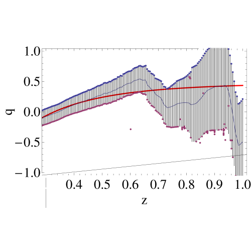
Daly & Djorgovski DD04 developed a numerical method for a direct determination of the expansion and acceleration rates, $H(z)$ and $q(z)$, from the data, using the dimensionless coordinate distance $y(z)$, without making any assumptions about the nature or evolution of the dark energy. They use the equation

$$-q(z)\equiv\ddot{a}a/\dot{a}^{2}=1\leavevmode\nobreak\ +\leavevmode\nobreak\ (1+z)\leavevmode\nobreak\ (dy/dz)^{-1}(d^{2}y/dz^{2})\,,$$ (41)

valid for $k=0$. Eq.(41) depends only upon the Friedman-Robertson-Walker line element and the relation $(1+z)=a_{0}/a(t)$. Thus, this expression for $q(z)$ is valid for any homogeneous and isotropic Universe in which $(1+z)=a_{0}/a(t)$, and it is therefore quite general and can be compared with any model to account for the acceleration of the Universe. This approach has the advantage to be model independent, but it introduces larger errors in the estimation of $q(z)$, since the numerical derivation is very sensitive to the size and quality of data. An additional problem is posed by the sparse and not complete coverage of the $z$-range of interest. Measurement errors are propagated in the standard way leading to estimated uncertainties of the fitted values. In Fig. (11), we compare the $q(z)$ obtained by Daly & Djorgovski from their full dataset with our best fit model.

Figure 11: The allowed region for $q(z)$, obtained by Daly & Djorgovski, from the full dataset (shadow area). An approximated polynomial corresponding to a $z$-window $\Delta z=0.6$ is shown with the black–thin solid line. With the black–thick dashed lines, it is shown the approximated polynomial fitted to the smoothed data at $\pm 1\sigma$ range, and corresponding to a $z$-window $\Delta z=0.4$. The red–solid line shows the deceleration function, $q(z)$ for our model, corresponding to the the best fit values.

IV.3 Growth of density perturbations and observational constraints from galaxies redshift surveys

A relevant consequence of the presence of a dominant form of dark energy in the Universe, in addition to its primary effect on the expansion rate, is to modify the gravitational assembly of matter from which the observed large-scale structure originated. In linear perturbation theory, it is possible to describe the growth of a generic small amplitude density fluctuation $\delta_{M}\equiv\delta\rho_{m}/\rho_{m}$ through a second-order differential equation peeb80 ; ma+al99 :

$$\ddot{\delta}_{m}+2H(t)\dot{\delta}_{m}-4\pi{\rm G}\rho_{m}\delta_{m}=0.$$ (42)

In Eq. (42), the dark energy enters through its influence on the expansion rate $H(t)$. We shall consider Eq. (42) only in the matter dominated era, when the contribution of radiation is really negligible. In our model, Eq.(42) assumes the form

$$\ddot{\delta}_{m}+2\dot{\delta}_{m}\frac{2}{3}\,\left(\frac{-2t\left(-1-8V_{0}^{2}+\cosh{\sqrt{3V_{0}}}\right)+\sqrt{3V_{0}}\sinh{\sqrt{3V_{0}}t}}{-1+t^{2}+8t^{2}V_{0}^{2}-t^{2}\cosh{\sqrt{3V_{0}}}+\cosh{\sqrt{3V_{0}}t}}\right)+$$

(43)

$$-\delta_{m}\left(\frac{2+V_{0}(3+16V_{0})-2\cosh{\sqrt{3V_{0}}}}{-1+t^{2}+8t^{2}V_{0}^{2}-t^{2}\cosh{\sqrt{3V_{0}}}+\cosh{\sqrt{3V_{0}}t}}\right)=0\,.$$ (44)

Eq. (IV.3) does not admit exact analytic solutions. However, since with our choice of normalization the whole history of the Universe is confined in the range $t\in[0,1]$, and since we choose $\omega\leq 1$, we can expand the trigonometric functions appearing in Eq. (IV.3) in series around $t=0$, obtaining an integrable differential equation, which is a Fuchsian differential equation which admits hypergeometric solutions. For the growing mode, we get

$$\delta_{+}\propto t^{2/3}\ _{2}F_{1}\left[-\frac{1}{3},\frac{7}{6},\frac{11}{6};-\frac{9t^{2}V_{0}^{2}}{24+36V_{0}+192V_{0}^{2}-24\cosh{\sqrt{3V_{0}}}}\right]\,.$$ (45)

We use such an exact solution to study the behavior of the solution for $t\simeq 0$, and, mainly, to set the initial conditions at $t=0$ and numerically integrate Eq. (IV.3) in the whole range $[0,1]$. From its solutions, we can define a linear growth rate $f$ that measures how rapidly structures are being assembled in the Universe as a function of cosmic time, or, equivalently, of the redshift:

$$f\equiv\frac{d\ln\delta_{+}}{d\ln a}\,,$$ (46)

where $a$ is the scale factor.

Figure 12: The growth index $f$ in our cosmological model (the solid line), compared with its functional dependence from $\Omega_{m}^{\gamma}(z)$, with $\gamma=0.55$ (dashed line).

Figure 13: The relative error between the growth index $f$ in our cosmological model $\Omega_{m}^{\gamma}(z)$, with $\gamma=0.55$: it turns out that such a relation describes quite well the linear growth rate.

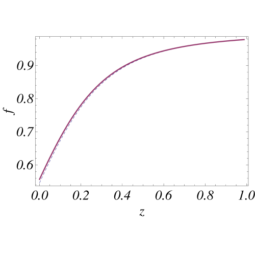
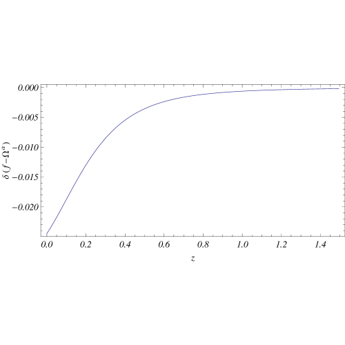
The growth index $f(z)$ essentially depends on the value of the mass density parameter at the given epoch, $\Omega_{m}$. For the cosmological-constant model the dependence is $f\propto\Omega_{m}^{0.55}$. However, this is not valid if the observed acceleration originates from a modification of the equations of General Relativity; for example, in the Dvali-Gabadadze-Porrati (DGP) braneworld theory DGP ; DGP2 ; DGP3 , an extra-dimensional modification of gravity gives $f(z)\propto\Omega_{m}^{0.68}(z)$. In general, a fitting form $f(z)f(z)\propto\Omega_{m}^{\gamma}(z)$ has been shown to be an accurate description for a wide range of models (for which $\Omega_{m}^{\gamma}(z)$ itself, not only $\gamma$, depends on the model). Thus, models with the same expansion history $H(z)$ but a different gravity theory, will have a different growth rate evolution $f(z)$ and index $\gamma$. A discrepancy between the measured value of the growth rate and that computed independently (assuming General Relativity) from the $H(z)$ yielded by SNeIa would point out modifications of gravity. In Figs. 12, 13, we show that, for the parameters of our model, the relation $f(z)\propto\Omega_{m}^{0.68}(z)$ works quite well. Some observational techniques have been suggested to measure $f(z)$ at different redshifts. Redshift-space distortions, that is, the imprint of large-scale peculiar velocities on observed galaxy maps, have not yet been considered in this context. Gravity driven coherent motions are in fact a direct consequence of the growth of structure. The anisotropy they induce in the observed galaxy clustering, when redshifts are used as a measure of galaxy distances, can be quantified by means of the redshift-space two-point correlation function $\xi(r_{p},pi)$,where $r_{p}$ and $\pi$ are respectively the transverse and line–of–sight components of galaxy separations. The anisotropy of $\xi(r_{p},pi)$ has a characteristic shape at large $r_{p}$ that depends on the parameter $\beta=\frac{f}{b_{L}}$. In practice, we observe a compression that is proportional to the growth rate, weighted by the factor $b_{L}$, the linear bias parameter of the specific class of galaxies being analyzed. The parameter $b_{L}$ measures how closely galaxies trace the mass density field, and is quantified by the ratio of the root-mean-square fluctuations in the galaxy and mass distributions on linear scales. A value of $\beta 0.49\pm 0.09$ has been measured at $z=0.15$ using the 2dF Galaxy Redshift Survey (2dFGRS) sample of 220,000 galaxies with bias ver+al01 ; la+al02 . From the observationally determined $\beta$ and $b$, it is now straightforward to get the value of the growth index at $z=0.15$ corresponding to the effective depth of the survey. Verde & al. (2001) used the bi-spectrum of 2dFGRS galaxies, and Lahav & al.  (2002) combined the 2dFGRS data with CMB data, and they obtained

$$b_{L_{verde}} = 1.04\pm 0.11\,,$$ (47)

$$b_{L_{lahav}} = 1.19\pm 0.09\,.$$ (48)

Using these two values for $b$ the value of the growth index $f$ at $z=0.15$ is

$$f_{1} = 0.51\pm 0.1\,,$$ (49)

$$f_{2} = 0.58\pm 0.11\,.$$ (50)

More recently, Guzzo et al. reported a measurement of $\beta=0.70\pm 0.26$ at a redshift of $0.77$, using new spectroscopic data from the Wide part of the VIMOS-VLT Deep Survey (VVDS) guzzo08 . Using a new survey of more than 10,000 faint galaxies, they also measured the anisotropy parameter $b_{L}=0.70\pm 0.26$, which corresponds to a growth rate of structure at that time of $f=0.91\pm 0.36$. This is consistent with our cosmological model, which gives $f(0.77)=0.97\pm 0.12$and $f(0.15)=0.68\pm 0.2$. However it is also consistent with standard $\Lambda$CDM with low matter density and flat geometry, although the error bars are still too large to distinguish among alternative origins for the accelerated expansion. This could be achieved with a further factor-of-ten increase in the sampled volume at similar redshift.

V Conclusions

We have investigated the possibility that phantom field dynamics could be derived by the Noether Symmetry Approach. The method allows to fix the self–interacting potential of the phantom field and then to solve exactly the field equations, at least in the case of dark energy and matter dominated Universe. The main cosmological parameters can be directly derived starting from the general solution. We also worked out a comparison between the theoretical predictions and observational dataset, as the publicly available data on SNeIa and radiogalaxies, the parameters of large scale structure determined from the 2-degree Field Galaxy Redshift Survey (2dFGRS)and from the Wide part of the VIMOS-VLT Deep Survey (VVDS). It turns out that the model is quite well compatible with the presently available observational data.

Furthermore, we extended the approach to the case including radiation. It can be shown that radiation is hardly changing the behavior of the scalar field, its potential, the Hubble constant and the $w$ parameter of the dark energy equation of state. As expected, the evolution of the $\Omega$ parameters is different. At the initial epochs, radiation dominates the expansion rate of the Universe, with dark energy and matter being sub-dominant. At a redshift of about 5000, the energy density of matter and radiation become almost equivalent and, for a relatively short period, the Universe becomes matter dominated. At a redshift of about $1$, dark energy starts to dominate the expansion rate of the Universe. It turned out that during the epoch of nucleosynthesis ($z\sim 10^{9}$) the energy density of the scalar field is much smaller than the energy density of radiation, and during such an epoch the kinetic terms in the scalar–field energy density vanishes, and the potential terms is constant. This meas that the dark-energy term acts as an effective cosmological constant $\Lambda$, and it does not influence the process of primordial nucleosynthesis.

As concluding remark, it is interesting to see that the presence of the Noether symmetry could constitute a physical criterion to fix the phantom potential. Such an approach revealed extremely useful also for other classes of models (see, e.g. defelice ; leandros ).

References

- (1) D.N.Spergel et al., ApJ Suppl. 170(2007) 377.
- (2) G. Hinshaw et al., ApJ Suppl. 170 (2007) 288.
- (3) L. Page et al., ApJ Suppl. 170 (2007) 335.
- (4) R.R. Caldwell, Phys. Lett. B 545 (2002) 23.
- (5) S.M. Carroll, M. Hofman, and M. Trodden, Phys. Rev. D 68 (2003) 023509; S.D.H. Hsu, A. Jenkins, and M.B. Wise, Phys. Lett. B 597 (2004) 270.
- (6) S. Nojiri, and S.D. Odintsov, Phys. Lett. B 595 (2004) 1; Phys. Rev. D 70 (2004) 103522.
- (7) S.W. Hawking, and G.F.R. Ellis, The Large-scale Structure of Space-time (Cambridge Univ. Press, 1999).
- (8) M. Visser, Lorentzian Wormholes (Springer, New York, 1996).
- (9) J.D. Barrow, Class. Quantum Grav. 21 (2004) L79 ; Class. Quantum Grav. 21 (2004) 5619; J.D. Barrow, and Ch. Tsagas, Class. Quantum Grav. 22 (2005) 1563; L. Fernandez-Jambrina, and R. Lazkoz, Phys. Rev. D 70 (2004) 121503.
- (10) M.P. Da̧browski, W. Godłowski, and M. Szydłowski, Intern. Journ. Mod. Phys. D 13 (2004) 1669.
- (11) J.D. Barrow, Nucl. Phys. B 310 (1988) 743.
- (12) M.D. Pollock, Phys. Lett. B 215 (1988) 635.
- (13) B. Boisseau, G. Esposito-Farése, D. Polarski, and A.A. Starobinsky, Phys. Rev. Lett. 85 (2000) 2236; A.A. Starobinsky, Grav. Cosmol. 6 (2000) 157.
- (14) M.Demianski, E.Piedipalumbo, C. Rubano, C. Tortora, Astron.Astrophys. 454 (2006) 55
- (15) A. Kehagias, and E. Kiritsis, JHEP 9911 (1999) 022.
- (16) T. Chiba, T. Okabe, and M. Yamaguchi, Phys. Rev. D 62 (2000) 023511.
- (17) A.K. Sanyal, Int. Jou. Mod. Phys. A, 22 (2007) 1301.
- (18) P.H. Frampton, Phys. Lett. B 557 (2003) 135.
- (19) P.H. Frampton, Phys. Lett. B 555 (2003) 139.
- (20) S.M. Carroll, M. Hoffman, and M. Trodden, Phys. Rev. D 68 (2003) 023509.
- (21) A. Melchiorri, L. Mersini, C.J. Odman, and M. Trodden, Phys. Rev. D 68 (2003) 043509.
- (22) L. Mersini, M. Bastero-Gil and P. Kanti, Phys. Rev. D64 (2001) 043508.
- (23) M. Bastero-Gil, P.H. Frampton and L. Mersini, Phys. Rev. D65 (2002) 106002.
- (24) M. Abdalla, S. Nojiri, and S. Odintsov, Class. Quantum Grav. 22 (2005) L35.
- (25) J.K. Erickson, R.R. Caldwell, P.J. Steinhardt, C. Armendariz-Picon, and V. Mukhanov, Phys. Rev. Lett. 88 (2002) 121301.
- (26) X. Li, and J. Hao, Phys. Rev. D69 (2004) 107303.
- (27) P. Singh, M. Sami, and N. Dadhich, Phys. Rev. D 68 (2003) 043501.
- (28) S. Nojiri, and D. Odintsov, Phys. Lett. B562 (2003) 147.
- (29) S. Nojiri, and D. Odintsov, Phys. Lett. B565 (2003) 1.
- (30) S. Nojiri, and D. Odintsov, Phys. Lett. B571 (2003) 1.
- (31) S. Nojiri, and S.D. Odintsov, Phys. Lett. B576 (2003) 5.
- (32) M. Szydłowski, W. Czaja, and A. Krawiec, Phys. Rev. E/bf 72 (2005) 036221.
- (33) V.K. Onemli, and R.P. Woodard, Class. Quantum Grav. 19 (2002) 4607; Phys. Rev. D 70 (2004) 107301; T. Brunier, V.K. Onemli, and R.P. Woodard, Class. Quantum Grav. 22 (2005) 59.
- (34) P.F. Gonzalez-Diaz, Phys. Rev. D 68 (2003) 021303; Phys. Rev. D 69 (2004), 063522; Phys. Lett. B 586 (2004), 1; P.F. Gonzalez-Diaz, and C.L. Sigüenza, Nucl. Phys. B 697 (2004) 363.
- (35) E.N. Saridakis, P. F. Gonzalez-Diaz, C.L. Siguenza, arXiv:0901.1213v2 [astro-ph.CO]
- (36) M.P. Da̧browski, ApJ 447(1995) 43.
- (37) M.P. Da̧browski, Phys. Rev. D 71 (2005) 103505.
- (38) M.P. Da̧browski, T. Stachowiak and M. Szydłowski, Phys. Rev. D 68(2003) 103519.
- (39) K.A. Meissner and G. Veneziano, Phys. Lett. B 267 (1991) 33; Mod. Phys. Lett. A 6 (1991) 1721.
- (40) J.E. Lidsey, D.W. Wands, and E.J. Copeland, Phys. Rep. 337 (2000) 343.
- (41) L.P. Chimento Phys. Rev. D65 (2002) 063517.
- (42) J.M. Aguirregabiria, L.P. Chimento, A.S. Jacubi, and R. Lazkoz, Phys. Rev. D 67 (2003) 083518.
- (43) L. P. Chimento, M. I. Forte, R. Lazkoz and M.G. Richarte Phys. Rev. D 79 (2009) 043502.
- (44) L.P. Chimento and R. Lazkoz, Gen. Relativ. Gravit. 40 (2008) 2543.
- (45) L.P. Chimento, F.P. Devecchi, M.I. Forte and G. M. Kremer, Class.Quant.Grav. 25 (2008) 085007.
- (46) L.P. Chimento L. P. and W. Zimdahl, Int. J. Mod. Phys. D17 (2008) 2229.
- (47) L.P. Chimento and D. Pavon Phys. Rev. D73 (2006) 063511.
- (48) L.P. Chimento and R. Lazkoz Class. Quantum Grav. 23 (2006) 3195.
- (49) L.P. Chimento Phys. Lett. B 633 (2006) 9.
- (50) M. Cataldo and L.P. Chimento, Int. J. Mod. Phys. D17 (2008) 1981.
- (51) L.P. Chimento and R. Lazkoz Int. J. Mod. Phys. D14 (2005) 587.
- (52) J.M. Aguirregabiria, L.P. Chimento and R. Lazkoz Phys. Rev. D70 (2004) 023509.
- (53) L.P. Chimento L. P. and R. Lazkoz Phys. Rev. Lett. 91 (2003) 211301.
- (54) G. Calcagni, Phys. Rev. D71 (2005) 023511.
- (55) J. Khoury et al, Phys. Rev. D 64 (2001) 123522; P.J. Steinhardt, and N. Turok, Phys. Rev. D 65 (2002) 126003; J. Khoury, P.J. Steinhardt, and N. Turok, Phys. Rev. Lett. 92 (2004) 031302.
- (56) J.E. Lidsey, Phys. Rev. D 70 (2004) 041302.
- (57) E.N. Saridakis, arXiv:0811.1333v2 [hep-th]
- (58) C. Ilie, T. Biswas, K. Freese, arXiv:0908.0991v1 [astro-ph.CO].
- (59) M. Szydlowski and M. Heller, Acta Phys. Pol. B 14 (1983) 571.
- (60) M. Szydlowski et al., Gen. Rel. Grav. 38 (2006) 795.
- (61) S. Capozziello, R. de Ritis, C. Rubano, P. Scudellaro, Riv. Nuovo Cim. 19 N 4 (1996) 1.
- (62) S. Capozziello, A. Stabile, A. Troisi, Class. Quant. Grav. 24 (2007) 2153.
- (63) S. Capozziello and A. De Felice, JCAP 0808 (2008) 016.
- (64) S. Capozziello, S. Nesseris, L. Perivolaropoulos, JCAP 0712(2007) 009.
- (65) C. Rubano, P. Scudellaro, Gen. Rel. Grav. 34 (2002) 307.
- (66) M. Demianski, C.Rubano, C. Tortora, Astron. Astrophys. 431 (2005) 27.
- (67) A.G. Riess et al., ApJ 659 (2007) 98.
- (68) A.G. Riess et al., ApJ 607 (2007) 665.
- (69) P. Astier et al., Astron. Astroph. 447 (2006) 31.
- (70) R.A. Daly, S.G. Djorgovski, ApJ 612 (2004) 652.
- (71) E.J. Guerra, R.A. Daly, L. Wan, ApJ 544 (2000) 659; R.A. Daly, E.J. Guerra, AJ, 124 (2002) 1831; S. Podariu, R.A. Daly, M.P. Mory, B. Ratra, ApJ 584 (2003) 577; R.A. Daly, S.G. Djorgovski, ApJ 597 (2003) 9.
- (72) R.A. Daly, S.G. Djorgovski, astro-ph.0512576 (2005).
- (73) W.L. Freedman et al., ApJ 553(2001) 47.
- (74) L.L.R. Williams, P. Saha, AJ 119 (2000) 439; V.F. Cardone, S. Capozziello, V. Re, E. Piedipalumbo, Astron. Astroph. 379 (2001) 72; V.F. Cardone, S. Capozziello, V. Re, E. Piedipalumbo, Astron. Astroph. 382 (2002) 792; C. Tortora, E. Piedipalumbo, V.F. Cardone, MNRAS, 354 (2004) 353; T. York, I.W.A. Browne, O. Wucknitz, J.E. Skelton, MNRAS 357 (2005) 124.
- (75) J.P. Hughes, M. Birkinshaw, ApJ 501 (1998) 1; R. Saunders et al., MNRAS 341 (2003) 937; R.W. Schmidt, S.W. Allen, A.C. Fabian, MNRAS 352 (2004) 1413.
- (76) A. Riess et al. ApJ 699 (2009) 539.
- (77) Peebles P.J.E., Large Scale Structure of the Universe, Princeton University Press, Princeton 1980.
- (78) Ma, C.P., Caldwell R. R., Bode P., Wang L., ApJ, 521 (1999) L1.
- (79) Dvali, G.R., Gabadadze G., Porrati M., Phys. Lett. B, 485 (2000) 208.
- (80) Dvali, G.R., Gabadadze, G., Kolanovic, M., Nitti, F., Phys. Rev. D 64 (2001) 084004.
- (81) Dvali, G.R., Gabadadze, G., Kolanovic, M., Nitti, F., Phys. Rev. D 64 (2002) 024031.
- (82) Verde L., Kamionkowski M., Mohr J. J., Benson A.J. MNRAS, 321 (2001) L7.
- (83) Lahav O., Bridle S. L., Percival W. J., & the 2dFGRS Team, MNRAS 333 (2002) 961.
- (84) Guzzo L. & al. Nature, 451 (2008) 541.