AFM pulling and the folding of donor-acceptor oligorotaxanes: phenomenology and interpretation

Abstract

The thermodynamic driving force in the self-assembly of the secondary structure of a class of donor-acceptor oligorotaxanes is elucidated by means of molecular dynamics simulations of equilibrium isometric single-molecule force spectroscopy AFM experiments. The oligorotaxanes consist of cyclobis(paraquat-p-phenylene) rings threaded onto an oligomer of 1,5-dioxynaphthalenes linked by polyethers. The simulations are performed in a high dielectric medium using MM3 as the force field. The resulting force vs. extension isotherms show a mechanically unstable region in which the molecule unfolds and, for selected extensions, blinks in the force measurements between a high-force and a low-force regime. From the force vs. extension data the molecular potential of mean force is reconstructed using the weighted histogram analysis method and decomposed into energetic and entropic contributions. The simulations indicate that the folding of the oligorotaxanes is energetically favored but entropically penalized, with the energetic contributions overcoming the entropy penalty and effectively driving the self-assembly. In addition, an analogy between the single-molecule folding/unfolding events driven by the AFM tip and the thermodynamic theory of first-order phase transitions is discussed and general conditions, on the molecule and the cantilever, for the emergence of mechanical instabilities and blinks in the force measurements in equilibrium isometric pulling experiments are presented. In particular, it is shown that the mechanical stability properties observed during the extension are intimately related to the fluctuations in the force measurements.

I Introduction

Unfolding and unbinding events in individual macromolecules can be computationally studied by means of “pulling” molecular dynamics (MD) simulations Izrailev et al. (1998); Heymann and Grubmüller (1999); Isralewitz et al. (2001). These calculations simulate recent single-molecule experiments in which a molecule (typically a protein or DNA) attached to a surface is mechanically unfolded by pulling it with optical tweezers or an atomic force microscope (AFM) tip attached to a cantilever Evans (2001); Liphardt et al. (2001); Bustamante et al. (2005); Ritort (2006). Such experiments show stress maxima that have been linked to the breaking of hydrogen bonds, providing insight into the secondary and tertiary structure of the macromolecules, and the dynamical processes involved in muscle contraction, protein folding, transcription, shape memory materials and many others.

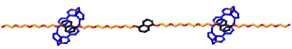
Figure 1: Structure of the [3]rotaxane. Oxygen atoms are depicted in red, the naphthalene units in black, and the polyether carbons in orange. The CBPQT⁴⁺rings are depicted in blue with the pyridinium N⁺ ions in brown.

In this paper we present simulations of single-molecule pulling for a class of donor-acceptor oligorotaxanes, as well as a detailed interpretation of the observed phenomenology. The pseudorotaxanes Amabilino and Stoddart (1995); Amabilino et al. (1995) considered consist of a variable number of cyclobis(paraquat-p-phenylene) tetracationic cyclophanes (CBPQT⁴⁺) threaded onto a linear chain composed of three naphthalene units linked by polyethers, with polyether caps at each end (see Fig. 1). These molecules have been recently synthesized by Basu et al. Basu et al. (To be published, 2009), and are oligomeric analogues of polyrotaxanes previously developed by the Stoddart group Zhang et al. (2008). The relevant interactions that drive the folding of this class of molecules have, in the absence of applied stress, been recently characterized Franco et al. (To be published, 2009). The interest in this paper is to investigate folding/unfolding pathways for these molecules under stress, and to determine, from a thermodynamic perspective, what drives the folding. In this sense, the AFM pulling setup is a valuable tool since it allows inducing unfolding/refolding events at the single-molecule level while simultaneously performing thermodynamic measurements.

The AFM pulling of the rotaxanes is simulated using constant temperature MD in a high dielectric medium using MM3 as the force field Allinger et al. (1989); Lii and Allinger (1989a, b). We focus on the isometric version of these experiments in which the distance between the surface and the cantilever is controlled while the force exerted is allowed to vary. Closely related experimental efforts are currently underway in the Stoddart group. To bridge the several orders of magnitude gap between the pulling speeds that are experimentally employed ($1-10^{-3}~{}\mu$m/s) and those that are computationally accessible, in the simulations the unfolding events are driven slowly enough that quasistatic behavior is recovered and the results become independent of the pulling speed.

A central quantity of interest in this analysis is the molecular potential of mean force (PMF) Zwanzig (1954) along the extension coordinate. The PMF is the Helmholtz free energy profile along a given reaction coordinate. As such, it succinctly captures the thermodynamic changes experienced by the molecule during the folding. Here, the PMF is reconstructed from the equilibrium force measurements using the weighted histogram analysis method (WHAM) Ferrenberg and Swendsen (1989); Kumar et al. (1992); Frenkel and Smit (2002). Related approaches based on nonequilibrium force measurements that exploit the Jarzynski Jarzynski (1997, 2008); Liphardt et al. (2002) and related equalities have been presented previously Hummer and Szabo (2001, 2005); Park and Schulten (2004); Harris et al. (2007); Imparato et al. (2008). Further insight into the thermodynamic driving force behind the folding is obtained by decomposing the PMF into energetic and entropic contributions.

In addition, an analogy between the phenomenology observed during the pulling of the rotaxanes and that expected for a system undergoing a first-order phase transition is presented. In the process of exploring such an analogy, several general features of the isometric pulling experiments will be revealed. Specifically, the dependence of the force vs. extension curves on the cantilever spring constant is characterized, and general conditions on the molecule and on the cantilever necessary for the emergence of mechanical instability and blinks in the force measurements are isolated. In particular, it is shown that the mechanical stability properties observed during the pulling are intimately related to the fluctuations in the force measurements. These results complement previous studies done by Kreuzer et al. Kreuzer and Payne (2001) in which the soft-spring and stiff-spring limit of the AFM pulling were identified with the Gibbs and Helmholtz ensembles for the isolated molecule, those of Kirmizialtin et al. Kirmizialtin et al. (2005) in which the origin of the dynamical bistability observed in constant force experiments Liphardt et al. (2001) and its relationship with the topography of the PMF was clarified, and those of Friddle et al. Friddle et al. (2008) in which the dependence of the rupture force on the cantilever spring constant was analyzed for a simple model potential meant to represent bond-breaking (see Ref. Freund, 2009 for an analysis of the bond survival probability). The conditions isolated below apply to any system subject to equilibrium isometric pulling using AFM tips attached to harmonic cantilevers.

This manuscript is organized as follows. In Sec. II.1 the protocol employed to simulate the isometric pulling of the rotaxanes is described. Sections II.2 and II.3 summarize, respectively, the strategy used to reconstruct the PMF from the force measurements and the procedure employed to decompose it into energetic and entropic contributions. Our main results are presented in Sec. III. Specifically, in Sec. III.1 the basic features observed during the mechanical unfolding of the oligorotaxanes are presented and the resulting PMF discussed. In Sec. III.2 the origin of the mechanical instabilities and blinks in the force measurements observed during the extension is clarified, and minimum conditions for the emergence of these effects are presented. Our main conclusions are summarized in Sec. IV.

II Theoretical Methodology

II.1 Pulling simulations

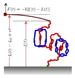
Figure 2: Schematic of an isometric single-molecule force spectroscopy experiment using an atomic force microscope (AFM). In it, one end of the molecular system is attached to a surface and the other end to an AFM tip attached to a cantilever. During the pulling, the distance between the surface and the cantilever $L(t)=L_{0}+vt$ is controlled and varied at a constant speed $v$. The deflection of the cantilever from its equilibrium position measures the instantaneous applied force on the molecule by the cantilever $F(t)=-k[\xi(t)-L(t)]$, where $k$ is the cantilever spring constant and $\xi(t)$ the fluctuating molecular end-to-end extension.

Unfolding of the rotaxanes is computationally studied by means of pulling MD simulations. The simulations are analogous to single-molecule force spectroscopy experiments in which a molecule attached to a surface is mechanically unfolded by pulling it with an AFM tip attached to a cantilever. The general setup of this class of experiments is shown in Fig. 2. The stretching computation begins by attaching one end of the molecule to a stiff isotropic harmonic potential that mimics the molecular attachment to the surface. Simultaneously, the opposite molecular end is connected to a dummy atom via a virtual harmonic spring. The position of the dummy atom is the simulation analogue of the cantilever position, and is controlled throughout. In turn, the varying deflection of the virtual harmonic spring measures the force exerted during the pulling. The stretching is caused by moving the dummy atom away from the molecule at a constant speed. The pulling direction is defined by the vector connecting the two terminal atoms of the complex. Since cantilever potentials are typically stiff in the direction perpendicular to the pulling, in the simulations the terminal atom that is being pulled is forced to move along the pulling direction by introducing appropriate additional harmonic restraining potentials. This type of simulations does not take into account any effects that may arise due to the interaction between the molecule and the AFM tip or the surface that cannot be accounted for by simple position restraints, nor any variations in the cantilever position due to thermal fluctuations or solvent-induced viscous drags.

The potential energy function of the molecule plus restraints is of the form

$$U_{L}(\boldsymbol{r})=U_{0}(\boldsymbol{r})+V_{L}[\xi(\boldsymbol{r}),t],$$ (1)

where $U_{0}(\boldsymbol{r})$ is the molecular potential energy plus potential restraints not varied during the simulation, $\boldsymbol{r}$ denotes the position of the $N$ atoms in the macromolecule, and

$$V_{L}[\xi(\boldsymbol{r}),t]=\frac{k}{2}\left[\xi(\boldsymbol{r})-L(t)\right]^{2}$$ (2)

is the potential due to the cantilever. Here $\xi(\boldsymbol{r})$ is the molecular end-to-end distance function, $L=L_{0}+vt$ is the distance from the cantilever to the surface at time $t$, $v$ is the pulling speed, and $k$ the cantilever spring constant. The force exerted by the cantilever on the molecule at time $t$ is given by

$$F(t)=-\nabla V_{L}=\frac{\partial V_{L}}{\partial L}=-k\left[\xi(\boldsymbol{r})-L(t)\right],$$ (3)

where the gradient $\nabla$ is with respect to the $[\xi(\boldsymbol{r})-L]$ coordinate. In writing Eqs. (2) and (3) the vector nature of $v(t)$, $L(t)$, $\xi(\boldsymbol{r})$ and $F(t)$ has been obviated since these quantities are collinear in the current setup.

The simulations are performed using Tinker 4.2 Ponder (2004) for which a pulling routine was developed. The stretching is performed using a soft cantilever potential with spring constant $k=0.011$ N/m $=1.1$ pN/Å. Since thermal fluctuations in the force depend on $k$ as $\delta F\sim\sqrt{k/\beta}$ Izrailev et al. (1998) (where $\beta=1/k_{\text{B}}T$ is the inverse temperature), such a soft spring constant provides high resolution in the force measurements. The macromolecules are described using the MM3 force field, which we have found adequately reproduces the complexation energies and the interactions responsible for the folding of the oligorotaxanes Franco et al. (To be published, 2009). As a simple model for the solvent, we use a continuum high dielectric medium in which the overall dielectric constant of the force field is set to that of water at room temperature (78.3). This is to be compared with the MM3 dielectric constant for vacuum of 1.5 Allinger et al. (1990). Any solvent effects that cannot be described using this continuum description are absent. The dynamics is propagated using a modified Beeman algorithm with a 1 fs integration time step, and the system is coupled to a heat bath at 300 K using a Nosé-Hoover chain as the thermostat. Initial –minimum energy– structures for the pulling simulations were obtained using simulated annealing, as described in Ref. Franco et al., To be published, 2009. These initial structures were allowed to equilibrate thermally for 1 ns and subsequently stretched. The simulations do not include counterions for the tetracationic cyclophanes since, at 300K and for the high dielectric medium employed, their interaction with the main molecular backbone is small and their effect on the folding negligible.

II.2 Reconstructing the PMF using WHAM

Under reversible conditions, knowledge of the force exerted during the pulling immediately yields the associated change in the Helmholtz free energy $A$ for the molecule plus cantilever. This is because the change in $A$ is determined by the reversible work exerted during the pulling

$$\Delta A=\int_{L_{0}}^{L}\langle F\rangle_{L^{\prime}}\,\mathrm{d}L^{\prime}=-\frac{1}{\beta}\ln\frac{Z(L)}{Z(L_{0})},$$ (4)

where $\langle F\rangle_{L}$ is the average force at extension $L$, and

$$Z(L)=\int\mathrm{d}\boldsymbol{r}\exp[-\beta U_{L}(\boldsymbol{r})]$$ (5)

is the configurational partition function of the molecule plus cantilever. Equation (4) follows from standard thermodynamic integration considerations Frenkel and Smit (2002), and assumes that at each point during the extension the state of the molecule plus cantilever potential is well described by a canonical ensemble. This property is expected for a system in weak contact with a thermal bath and is enforced in the simulations by the nature of the thermostat employed.

From the force versus extension measurements it is also possible to extract the molecular potential of mean force (PMF) $\phi(\xi)$ as a function of the end-to-end distance $\xi$ by properly removing the bias due to the cantilever potential. The quantity $\phi(\xi)$ is the Helmholtz free energy profile along the coordinate $\xi$ for the isolated (cantilever-free) molecule, and is of central interest since it succinctly characterizes the thermodynamics of the unfolding. Below we summarize how to estimate this quantity from the force measurements employing the weighted histogram analysis method (WHAM).

The PMF is defined by Roux (1995)

$$\phi(\xi)=\phi(\xi^{\star})-\frac{1}{\beta}\ln\left[\frac{p_{0}(\xi)}{p_{0}(\xi^{\star})}\right],$$ (6)

where $\xi^{\star}$ and $\phi(\xi^{\star})$ are arbitrary constants and

$$p_{0}(\xi)=\frac{\int\mathrm{d}\boldsymbol{r}\,\delta[\xi-\xi(\boldsymbol{r})]\exp[-\beta U_{0}(\boldsymbol{r})]}{\int\mathrm{d}\boldsymbol{r}\,\exp[-\beta U_{0}(\boldsymbol{r})]}=\frac{Z_{0}(\xi)}{Z_{0}}=\langle\delta[\xi-\xi(\boldsymbol{r})]\rangle.$$ (7)

Here,

$$Z_{0}=\int\mathrm{d}\boldsymbol{r}\,\exp[-\beta U_{0}(\boldsymbol{r})]$$ (8)

is the configurational partition function of the molecule, and

$$Z_{0}(\xi)=\int\mathrm{d}\boldsymbol{r}\,\delta[\xi-\xi(\boldsymbol{r})]\exp[-\beta U_{0}(\boldsymbol{r})].$$ (9)

In the context of the pulling experiments $p_{0}(\xi)$ is the probability density that the molecular end-to-end distance function $\xi(\boldsymbol{r})$ adopts the value $\xi$ in the unbiased (cantilever-free) ensemble. The quantity $p_{0}(\xi)$ determines the PMF up to a constant and can be estimated from the force measurements, as we now describe.

At this point it is convenient to discretize the time variable during the pulling experiment into $M$ steps: $t_{1},\ldots,t_{i},\ldots,t_{M}$. The potential of the system plus cantilever at time $t_{i}$ is $U_{i}=U_{0}+V_{i}$, where $V_{i}=\frac{k}{2}[\xi(\boldsymbol{r},t_{i})-L(t_{i})]^{2}$ is the bias due to the cantilever potential. In the $i$-th biased measurement knowledge of the force $F_{i}$ and $L(t_{i})$ gives the molecular end-to-end distance. The probability density of observing the value $\xi$ at this time is given by

$$p_{i}(\xi)=\frac{\int\mathrm{d}\boldsymbol{r}\,\delta[\xi-\xi(\boldsymbol{r})]\exp[-\beta U_{i}(\boldsymbol{r})]}{\int\mathrm{d}\boldsymbol{r}\,\exp[-\beta U_{i}(\boldsymbol{r})]}=\frac{Z_{i}(\xi)}{Z_{i}}=\langle\delta[\xi-\xi(\boldsymbol{r})]\rangle_{i},$$ (10)

where $Z_{i}=\int\mathrm{d}\boldsymbol{r}\,\exp[-\beta U_{i}(\boldsymbol{r})]$ is the configurational partition function for the system plus cantilever at the $i$-th extension, and

$$Z_{i}(\xi)=\int\mathrm{d}\boldsymbol{r}\delta[\xi-\xi(\boldsymbol{r})]\exp[-\beta U_{i}(\boldsymbol{r})].$$ (11)

Knowledge of $p_{i}(\xi)$ allows the unbiased probability density $p_{0}(\xi)$ to be reconstructed since, by virtue of Eqs. (7) and (10), these two quantities are related by

$$p_{0}(\xi)=\exp[+\beta V_{i}(\xi)]\frac{Z_{i}}{Z_{0}}p_{i}(\xi),$$ (12)

where we have exploited the fact that $Z_{0}(\xi)=\exp[+\beta V_{i}(\xi)]Z_{i}(\xi)$. In the pulling experiments, for each $L(t_{i})$ only a few force measurements are typically performed and the probability density $p_{i}(\xi)$ is not properly sampled. Nevertheless, the experiments do provide measurements at a wealth of values of $L(t_{i})$ that can be combined to estimate $p_{0}(\xi)$:

$$p_{0}(\xi)=\sum_{i=1}^{M}w_{i}\exp[+\beta V_{i}(\xi)]\frac{Z_{i}}{Z_{0}}p_{i}(\xi),$$ (13)

where the $w_{i}$ are some normalized ($\sum_{i}w_{i}=1$) set of weights. In the limit of perfect sampling any set of weights should yield the same $p_{0}(\xi)$. In practice, for finite sampling it is convenient to employ a set that minimizes the variance in the $p_{0}(\xi)$ estimate from the series of independent estimates of biased distributions. Such a set of weights is precisely provided by the WHAM prescription Ferrenberg and Swendsen (1989); Kumar et al. (1992); Frenkel and Smit (2002); Chodera et al. (2007)

$$w_{i}=\frac{\exp[-\beta V_{i}(\xi)]\dfrac{Z_{0}}{Z_{i}g_{i}}}{\sum_{i=1}^{M}\exp[-\beta V_{i}(\xi)]\dfrac{Z_{0}}{Z_{i}g_{i}}},$$ (14)

where $g_{i}=1+2\tau_{i}$ is the statistical inefficiency Chodera et al. (2007) and $\tau_{i}$ the integrated autocorrelation time Ferrenberg and Swendsen (1989); Chodera et al. (2007). The difficulty in estimating the $\tau_{i}$ for each measurement generally leads to further supposing that the $g_{i}$’s are approximately constant and factor out of Eq. (14), so that

$$p_{0}(\xi)=\frac{\sum_{i=1}^{M}p_{i}(\xi)}{\sum_{i=1}^{M}\exp[-\beta V_{i}(\xi)]Z_{0}/Z_{i}}.$$ (15)

Neglecting the $g_{i}$’s from Eq. (15) does not imply that the resulting estimate of $p_{0}(\xi)$ is incorrect; but simply that the weights selected do not precisely minimize the variance in the estimate. Experience with this method indicates that if the $g_{i}$’s do not differ by more than an order of magnitude their effect on $\phi(\xi)$ is small Kumar et al. (1992).

The computation of the PMF then proceeds as follows. Suppose that $N_{i}$ force measurements are done for each extension $i$. Knowledge of the force $F_{i}^{j}$ ($j=1,\ldots,N_{i}$) and of $L(t_{i})$ gives the molecular end-to-end distance $\xi_{i}^{j}$ in each of these measurements. The numerator in Eq. (15) is then estimated by constructing a histogram with all the available data,

$$\sum_{i=1}^{M}p_{i}(\xi)\approx\sum_{i=1}^{M}\sum_{j=1}^{N_{i}}\frac{C_{i}^{j}(\xi)}{N_{i}\Delta\xi},$$ (16)

where $\Delta\xi$ is the bin size, and $C_{i}^{j}(\xi)=1$ if $\xi_{i}^{j}\in[\xi-\Delta\xi/2,\xi+\Delta\xi/2)$ and zero otherwise. Estimating the denominator in Eq. (15) requires knowledge of the $Z_{i}$’s, the configurational partition functions of the system plus cantilever at all extensions $\{L(t_{i})\}$ considered. There are two ways to obtain these quantities. The most direct one is to employ the Helmholtz free energies for the system plus cantilever obtained through the thermodynamic integration in Eq. (4), as they determine the $Z_{i}$’s up to a constant multiplicative factor. Alternatively, it is also possible to determine the ratio of the configurational partition functions between the $i$-th biased system and its unbiased counterpart using $p_{0}(\xi)$:

$$\frac{Z_{i}}{Z_{0}}=\int\mathrm{d}\xi\,\exp[-\beta V_{i}(\xi)]p_{0}(\xi).$$ (17)

Equations (15) and (17) can be solved iteratively. Starting from a guess for the $Z_{i}/Z_{0}$, $p_{0}(\xi)$ is estimated using Eq. (15) and normalized. The resulting $p_{0}(\xi)$ is then used to obtain a new set of $Z_{i}/Z_{0}$ through Eq. (17), and the process is repeated until self-consistency. This latter approach is the usual procedure to solve the WHAM equations. Note, however, that this procedure is not required if reversible force vs. extension data is available.

The reconstruction of the PMF from the force vs. extension measurements using WHAM is simple to implement. Further, the procedure is versatile in the sense that it makes no assumption about the stiffness of the cantilever potential and permits the combination of data from several pulling runs. In addition, as we describe below, it can also be employed to decompose the PMF into entropic and energetic contributions from data readily available from an MD run.

II.3 Energy-entropy decomposition of the PMF

Insight into the thermodynamic driving force responsible for the folding of oligorotaxanes can be obtained by decomposing the changes in the PMF into entropic $S(\xi)$ and potential energy $U_{0}(\xi)$ contributions,

$$\phi(\xi)-\phi(\xi^{*})=\left[U_{0}(\xi)-U_{0}(\xi^{\star})\right]-T\left[S(\xi)-S(\xi^{*})\right].$$ (18)

Here,

$$U_{0}(\xi)=\frac{1}{Z_{0}(\xi)}\int\mathrm{d}\boldsymbol{r}\,\delta[\xi-\xi(\boldsymbol{r})]U_{0}(\boldsymbol{r})\exp[-\beta U_{0}(\boldsymbol{r})]$$ (19)

is the average potential energy when the end-to-end distance adopts the value $\xi$, and

$$TS(\xi)=-\frac{1}{\beta\Omega_{0}}\int\mathrm{d}\boldsymbol{r}\,\delta[\xi-\xi(\boldsymbol{r})]\rho\ln\rho$$ (20)

is the corresponding configurational entropy, where $\rho=\frac{\Omega_{0}}{Z_{0}(\xi)}\exp[-\beta U_{0}(\boldsymbol{r})]$ and $\Omega_{0}$ is a constant irrelevant factor with the same dimensions as $Z_{0}(\xi)$. Equation (18) follows from the above definitions.

The energy-entropy decomposition of the PMF can be obtained by estimating $U_{0}(\xi)$ directly and employing the previously reconstructed $\phi(\xi)$ to obtain $TS(\xi)$ using Eq. (18). Here, $U_{0}(\xi)$ is estimated by combining all measurements performed during the pulling simulations using WHAM. The measurable quantity in the simulation in the presence of the bias due to the cantilever is:

$$\langle U_{0}(\boldsymbol{r})\delta[\xi-\xi(\boldsymbol{r})]\rangle_{i}=\frac{\int\mathrm{d}\boldsymbol{r}\,\delta[\xi-\xi(\boldsymbol{r})]U_{0}(\boldsymbol{r})\exp[-\beta U_{i}(\boldsymbol{r})]}{Z_{i}},$$ (21)

the average molecular potential energy when the end-to-end distance adopts the value $\xi$ and the cantilever extension is $L(t_{i})$. This average in the biased ensemble is related to the unbiased average $U_{0}(\xi)$ by:

$$U_{0}(\xi)=\exp[+\beta V_{i}(\xi)]\frac{Z_{i}}{Z_{0}(\xi)}\langle U_{0}(\boldsymbol{r})\delta[\xi-\xi(\boldsymbol{r})]\rangle_{i}.$$ (22)

As in the estimation of $p_{0}(\xi)$, all data collected during pulling can be combined with appropriate weights $w_{i}$ to estimate $U_{0}(\xi)$,

$$U_{0}(\xi)=\sum_{i=1}^{M}w_{i}\exp[+\beta V_{i}(\xi)]\frac{Z_{i}}{Z_{0}(\xi)}\langle U_{0}(\boldsymbol{r})\delta[\xi-\xi(\boldsymbol{r})]\rangle_{i}.$$ (23)

If one adopts the weights $w_{i}$ that define the WHAM prescription [Eq. (14)], then

$$U_{0}(\xi)=\frac{\sum_{i}\langle U_{0}(\boldsymbol{r})\delta[\xi-\xi(\boldsymbol{r})]\rangle_{i}}{\sum_{i}\exp[-\beta V_{i}(\xi)]Z_{0}(\xi)/Z_{i}},$$ (24)

where we have assumed identical statistical inefficiencies for all $i$. Last, recalling the definition of $p_{0}(\xi)=Z_{0}(\xi)/Z_{0}$ [Eq. (7)] and its WHAM prescription [Eq. (15)], one arrives at a useful expression for $U_{0}(\xi)$,

$$U_{0}(\xi)=\frac{\sum_{i}\langle U_{0}(\boldsymbol{r})\delta[\xi-\xi(\boldsymbol{r})]\rangle_{i}}{\sum_{i}\langle\delta[\xi-\xi(\boldsymbol{r})]\rangle_{i}}.$$ (25)

Equation (25) provides a mean to calculate the potential energy as a function of the end-to-end distance by combining all the data obtained during the pulling. The remarkable simplicity of Eq. (25) is noteworthy: in order to obtain $U_{0}(\xi)$ one just needs to generate histograms for the the values of $\xi$ observed using all data collected during the pulling and then, within each bin, perform a simple average of the internal energy of the configurations that fall into it. It does not require knowledge of the properties of the bias potential.

This method of performing an energy-entropy decomposition of the PMF requires knowledge of $U_{0}(\xi)$ for the configurations observed during pulling. This quantity, although readily available in an MD run, is not experimentally accessible. As a result, in experiments an energy-entropy decomposition of the PMF requires estimating the changes in entropy by performing the pulling at varying temperatures.

III Results and discussion

III.1 Phenomenology of the pulling experiments

III.1.1 The approach to equilibrium

One of the challenges in simulating AFM pulling experiments using MD is to bridge the large disparity between the pulling speeds $v$ that are employed experimentally and those that can be accessed computationally. While typical experiments often use $v\sim 1-10^{-3}$ $\mu$m/s, current computational capabilities require pulling speeds that are several orders of magnitude faster. Here, this difficulty is circumvented by striving for pulling speeds that are slow enough that reversible behavior is recovered. Under such conditions the results become independent of $v$, and the simulations comparable to experimental findings.

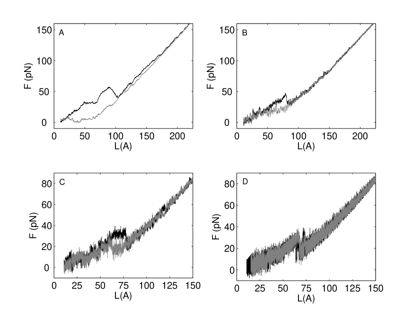
Figure 3: The approach to equilibrium in the pulling simulations. The figure shows force vs. extension profiles for the [3]rotaxane immersed in a high dielectric medium at 300K for different pulling speeds $v$ of (A) $10^{0}$, (B) $10^{-1}$, (C) $10^{-2}$ and (D) $10^{-3}$ Å/ps. The harmonic cantilever employed has a soft spring constant of $k=0.011$ N/m, $L$ is the distance between the surface and the cantilever and $F$ the instantaneous applied force. The black lines correspond to the extension process; the gray ones to the contraction.

Consider the pulling of the [3]rotaxane shown in Fig. 1 (the simulation details are specified in Sec. II.1). Figure 3 shows the effect of decreasing the pulling speed on the force vs. extension characteristics. In the simulations, the system is first extended (black lines) to a given $L$ and then contracted (gray lines). For pulling speeds (and equal retracting speeds) between $1-0.01$ Å/ps (panels A to C) hysteresis and other nonequilibrium effects during the pulling are unavoidable. However, for $v=0.001$ Å/ps $=10^{5}$ $\mu$m/s the system behaves reversibly, and the $F$-$L$ curves obtained during extension and contraction essentially coincide. Note the second law of thermodynamics at play in the simulations: the work required to stretch the molecule –the area under the curve– decreases with the pulling speed until reversible behavior is attained. We have observed that pulling speeds of $\sim 10^{-3}$ Å/ps are generally sufficient to recover reversible behavior for the unfolding in a high dielectric medium of the [n]rotaxanes considered. For simulations in vacuum slower pulling speeds are required.

It is worth noting that this seemingly simple phenomenological behavior is not recovered when a Berendsen thermostat is employed instead of a Nosé-Hoover chain. In fact, we have observed that the Berendsen thermostat leads to a spurious violation of the second law during the pulling, presumably because the ensemble generated by it does not satisfy the equipartition theorem Harvey et al. (1998).

III.1.2 Reversible unfolding, mechanical instability and blinks in the force measurements

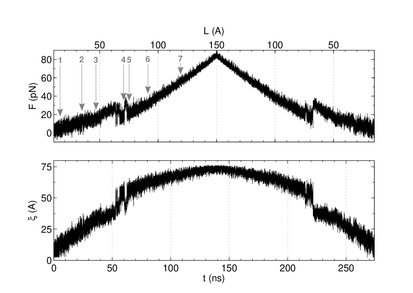
Figure 4: Time dependence of the force $F$ and the molecular end-to-end distance $\xi$ during the pulling of the [3]rotaxane under equilibrium conditions ($v=0.001$ Å/ps, $k=0.011$ N/m). Typical structures (labels 1-7) observed during the extension are shown in Fig. 5.

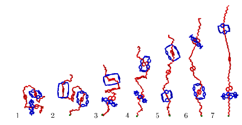
Figure 5: Snapshots of the [3]rotaxane during its extension. The numerical labels shown here are employed in Figs. 4,6 and 9.

Figure 4 details the force exerted (upper panel) and the molecular end-to-end distance (lower panel) during the reversible pulling and contraction of the [3]rotaxane. Snapshots of typical structures encountered during the pulling are included in Fig. 5. As the system is stretched the oligorotaxane undergoes a conformational transition from a folded globular state to an extended coil. In the process, the force initially increases approximately linearly with $L$, then drops, and subsequently increases again. The drop in the force is due to the unfolding of the rotaxane during the stretching.

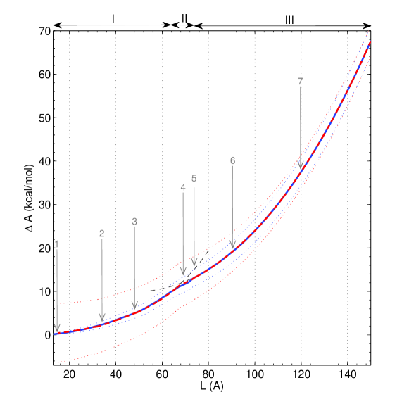
Figure 6: Changes in the Helmholtz free energy $A$ of the [3]rotaxane plus cantilever obtained from the data shown in Fig. 4. The blue line corresponds to the pulling and the red one to the contraction. The dotted lines provide an estimate of errors in the thermodynamic integration due to force fluctuations at each pulling step. The difference in the degree of convexity of regions I and III is evidenced by extrapolating the data in each region outside of its domain through fitting to quartic polynomials (black dashed lines). The labels correspond to the structures shown in Fig. 5.

Figure 6 shows the change in the Helmholtz free energy $A$ for the molecule plus cantilever obtained from integrating directly the $F$-$L$ curve in Fig. 4. The net change in free energy for the complete thermodynamic cycle is zero, as expected for a quasistatic process. The free energy profile for the system plus cantilever has three distinct regions, labeled I-III in the figure. Regions I and III correspond to the folded and extended state, respectively, while region II is where the folding/unfolding event occurs. From a thermodynamics perspective Callen (1985), regions I and III are mechanically stable phases since $A$ is a convex function of the extension $L$, i.e. $\left(\frac{\partial^{2}A}{\partial L^{2}}\right)_{T}=\left(\frac{\partial\langle F\rangle_{L}}{\partial L}\right)_{T}\geq 0$. By contrast, region II, where the unfolding occurs, is mechanically unstable since $A$ is a concave function of $L$ and hence $\left(\frac{\partial^{2}A}{\partial L^{2}}\right)_{T}=\left(\frac{\partial\langle F\rangle_{L}}{\partial L}\right)_{T}<0$.

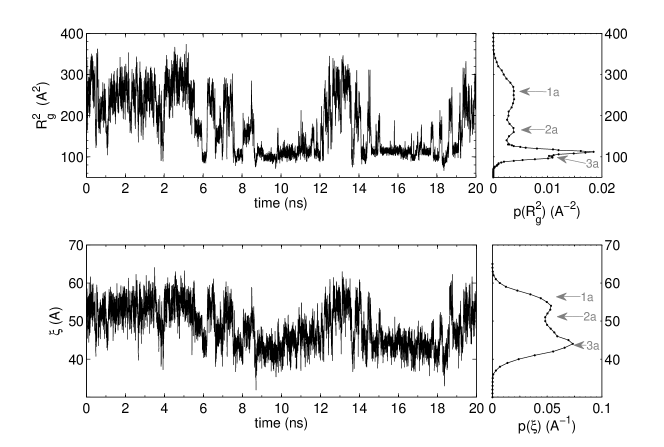
Figure 7: Time dependence and probability density distribution of the radius of gyration ($R_{g}^{2}$) and the end-to-end molecular extension $\xi$ when the [3]rotaxane plus cantilever is constrained to reside in the unstable region (II) of Fig. 6, with $L=70.0$ Å. Typical structures encountered in this regime (labels 1a-3a) are shown in Fig. 8.

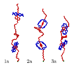
Figure 8: Structures observed in the unstable region of the pulling simulations. The numerical labels are employed in Fig. 7.

The dynamical behavior of the system in the unstable region is illustrated in Fig. 7, which shows the evolution of the radius of gyration $R_{g}$ and the molecular end-to-end distance when $L=70.0$ Å. In this region, the [3]rotaxane undergoes transitions between a folded globular state, partially folded structures, and an extended coil. The right panels in Fig. 7 show the probability density of the distribution of $R_{g}^{2}$ and $\xi$ values obtained from a 20 ns trajectory. The system exhibits a clear dynamical bistability along the $\xi$ coordinate, and at least a tristability along $R_{g}^{2}$. Figure 8 shows some representative structures encountered during this dynamics. The bistability along the end-to-end distance leads to a blinking in the force measurements from a high force to a low force regime during the pulling (cf. the unstable region in Fig. 4). The blinking in the force measurements in the isometric experiments is analogous to the blinking in the molecular extension observed during the constant force reversible pulling of single RNA molecules Liphardt et al. (2001). Note that for the cantilever stiffness employed this multistable behavior in the radius of gyration, or the end-to-end distance, is not observed when $L$ is set to be in the stable regions (I or III) of the free energy profile. The origin of the bistability along the end-to-end distance, the multistability in the radius of gyration, and its relation to the thermodynamic instability in the pulling is discussed in Sec. III.2.

III.1.3 The PMF and the thermodynamic driving force in the folding

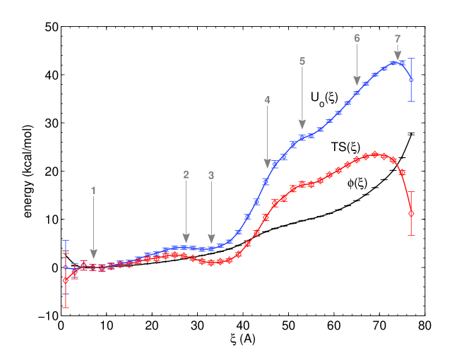
Figure 9: Potential $U_{0}(\xi)$ and entropic $TS(\xi)$ contributions to the PMF [Eq. (18)] of the [3]rotaxane along the end-to-end distance $\xi$. The results are averages of three different pulling simulations. The error bars correspond to twice the standard deviation obtained from a bootstrapping analysis. The solid lines result from a spline interpolation of the available data points. Typical structures (labels 1-7) are shown in Fig. 5.

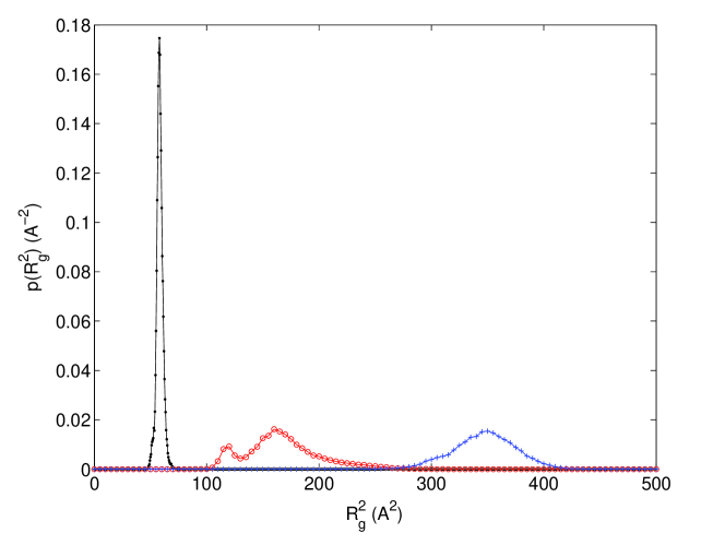
Figure 10: Probability density distribution of the radius of gyration $p(R_{g}^{2})$ for the [3]rotaxane when $\xi$ is fixed at 7.0 Å (dots), 47 Å (open circles) and 64.9 Å (crosses). Note the bistability along $R_{g}^{2}$ when $\xi$ is fixed at the concave region of the PMF.

Figure 9 shows the potential of mean force along the end-to-end distance $\xi$ for the [3]rotaxane reconstructed from the force measurements as described in Sec. II.2, as well as its decomposition into entropic and potential energy contributions. The thermodynamic native state of the oligorotaxane, i.e. the minimum in $\phi$, corresponds to a globular folded structure with $\xi_{0}=7$ Å. The structure of the molecular free energy profile as a function of $\xi$ is similar to that observed for the molecule plus cantilever as a function of $L$. Namely, it consists of a folded and an unfolded stable branch where $\phi(\xi)$ is a convex function, and a concave region around $\xi=44-52$ Å  where the conformational transition occurs. As discussed in Sec. III.2, this characteristic structure of the PMF is responsible for many of the interesting features observed during pulling. Figure 10 shows the probability distribution for $R_{g}^{2}$ at values of $\xi$ in the three main regions of the PMF, each collected during a 20 ns trajectory. In the stable regions ($\xi=7.0$ and 64.9 Å ), the evolution of the radius of gyration reveals only one stable structural state. By contrast, in the unstable region ($\xi=47$ Å) the distribution of $R_{g}^{2}$ values indicates that there is a inherent bistability in the molecular potential along the $R_{g}^{2}$ coordinate. Such molecular bistability gives rise to the region of concavity in the PMF.

What drives the folding of the oligorotaxanes from a thermodynamic perspective? The energy-entropy decomposition of the PMF indicates that the folding of the rotaxane is energetically favored but entropically penalized, with the energetic contributions overcoming the entropy penalty and effectively driving the self-assembly. Further, while the potential energy and the entropy of the molecule show considerable changes during the unfolding, these two effects largely cancel one another, leading to only modest changes in the Helmholtz free energy. Note that while $\phi(\xi)$ is a monotonic function of $\xi$ for $\xi>\xi_{0}$, the energy and entropy contributions show a clear nonmonotonic dependence on $\xi$. For instance, there is a reduction in the system’s entropy for $\xi$ both just before the conformational transition and for large extensions due to a reduction in the available degenerate conformational space.

It is important to stress that the PMF and its decomposition into energy and entropy contributions correspond to a molecule in which the terminal atoms are constrained to move along the pulling coordinate. As a consequence, any additional contributions that may arise by relaxing these constraints are simply not manifest in this picture of the folding.

III.1.4 Dependence of the PMF on the number of threaded rings

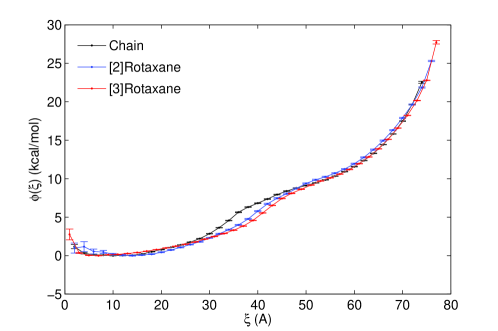
Figure 11: PMF as a function of the molecular extension $\xi$ extracted from force measurements using WHAM for rotaxanes with different numbers of threaded rings. The error bars correspond to twice the standard deviation obtained from a bootstrapping analysis.

Figure 11 compares the PMF extracted from force measurements for the [3]rotaxane, and the associated [2]rotaxane and bare molecular thread. In the [2]rotaxane system the CBPQT⁴⁺ring encircles the central naphthalene unit of the underlying chain. The PMF in all cases is qualitatively similar: it consists of two stable convex regions, and a unstable concave region where the unfolding occurs. Further, for all species the folding along $\xi$ is energetically driven and entropically penalized (not shown). Note that, in the high dielectric medium employed, the number of threaded rings does not have a dramatic effect on the net change in the free energy undergone during folding nor, as expected, on the elastic properties of the extended state. It does, however, have an appreciable effect on the stability and elasticity of the folded conformation. Specifically, as the number of rings is increased the range of $\xi$ values for which the folded conformation is stable increases. That is, a larger $L$ is required during the pulling to unfold the rotaxanes with respect to the bare chain.

III.2 Interpretation of the pulling experiments

III.2.1 Analogy with first-order phase transitions

At first glance, the phenomenological behavior observed by the molecule plus cantilever during the extension is analogous to that expected for a system undergoing a first-order phase transition Callen (1985). Namely, during the extension the combined system goes from one stable thermodynamic phase to another (Regions I and III in Fig. 6) by varying an externally controllable parameter, in this case $L$. In the transition region the Helmholtz free energy of the combined system is concave and, hence, fails to satisfy the thermodynamic stability criteria (Region II in Fig. 6). As a consequence, the observed $F$-$L$ isotherm (Fig. 4) exhibits a region of mechanical instability where $\left(\frac{\partial\langle F\rangle_{L}}{\partial L}\right)_{T}<0$. These observations largely parallel the behavior of unstable $P$-$V$ isotherms for a van der Waals fluid.

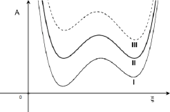
Figure 12: Schematic variation of the Helmholtz potential of the molecule plus cantilever as a function of $\xi$ for different extensions $L$ suggested by the phenomenological observations around the region of mechanical instability. The labels I-III correspond to the different stability regions in Fig. 6

In addition, the phenomenology seems to indicate that close to the transition region the Helmholtz potential for the molecule plus cantilever is bistable along the end-to-end distance, and has the characteristic form exhibited during a first-order phase transition schematically shown in Fig. 12. For $L\in$ Region I the stable global minimum corresponds to the molecule in a folded state, and as $L$ is increased the equilibrium state shifts from one local minimum to the other. For $L\in$ Region II the two minima become approximately equal and a transition from the folded state to the unfolded state occurs. Beyond this extension the unfolded molecular phase becomes the global potential minimum and the extended phase becomes absolutely stable. This interpretation is consistent with the observed behavior in which the system blinks between a folded and an extended state around the transition region, recall Fig. 7.

Note, however, that this analogy can never be completely faithful since the modeled single-molecule pulling experiment does not deal with a macroscopic system. This contrasts with the elastic behavior observed for polymer chains Halperin and Zhulina (1991); Gunari et al. (2007), and leads to salient differences between the two processes. First, while in a true first-order phase transition the physical system exhibits coexistence between the stable phases, in this single-molecule version no coexistence is possible. At the transition point, and for the value of $k$ employed, the system instead exhibits frequent jumps between the stable phases (cf. Fig. 7). Coexistence is replaced by ergodicity in this single-molecule manifestation of bistability. Second, the variable that is varied during the extension $L$ is not a true thermodynamic variable since it is neither extensive nor intensive. Third, the system considered has no clear thermodynamic limit in which a true discontinuity of the derivatives of the partition function can develop and, further, the system is far from the thermodynamic limit since the fluctuations observed in the $F$-$L$ curves are comparable to the average value, leading to a nonequivalence between statistical ensembles Hill (1983); Rubi et al. (2006). Additionally, the mechanical properties measured during the pulling are for the molecule plus cantilever, and hence the extension behavior is expected to depend on the nature of the cantilever.

Nevertheless, the similarities between the two processes are still intriguing and, in view of these observations, it is natural to ask: (i) what is the origin of the mechanical instability during the pulling?; (ii) how does the dynamical bistability along the end-to-end distance arise?; (iii) how does the nature of the cantilever affect the observed phenomenological behavior; and (iv) which features of the observed behavior arise due to the molecule, and which due to the cantilever? These questions are addressed in the following sections.

The key quantity in the remainder of this analysis is the PMF along the end-to-end distance [Eq. (6)]. Its utility relies on the fact that the configurational partition function of the molecule plus cantilever at extension $L$ [Eq. (5)] can be expressed as

$$Z(L)=\int\mathrm{d}{\xi}\,\exp\{-\beta[\phi(\xi)+V_{L}(\xi)]\},$$ (26)

where we have neglected the constant and $L$-independent multiplicative factor that arises in the transformation since it is irrelevant for the present purposes. The above relation implies that the extension process can be viewed as thermal motion along a one-dimensional effective potential determined by the PMF $\phi(\xi)$ and the bias due to the cantilever $V_{L}(\xi)$:

$$U_{L}(\xi)=\phi(\xi)+V_{L}(\xi).$$ (27)

Further, by means of the PMF it is possible to estimate the force vs. extension characteristics for the composite system for any value of the force constant $k$. This is because the average force exerted on the system at extension $L$ can be expressed as:

$$\langle F\rangle_{L}=-\frac{1}{\beta}\frac{\partial\ln[Z(L)/Z_{0}]}{\partial L}=\frac{\int\mathrm{d}\xi\,\frac{\partial V_{L}(\xi)}{\partial L}\exp\{-\beta[\phi(\xi)+V_{L}(\xi)]\}}{\int\mathrm{d}\xi\,\exp\{-\beta[\phi(\xi)+V_{L}(\xi)]\}},$$ (28)

where, for convenience, we have introduced $Z_{0}$ in the logarithm just to make the argument dimensionless. Since $\phi(\xi)$ is a property of the isolated molecule it is independent of $k$. Hence, Eq. (28) can be employed to estimate the $F$-$L$ isotherms for arbitrary $k$.

III.2.2 Dependence of the $F$-$L$ isotherms on the cantilever spring constant

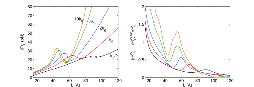
Figure 13: Left panel: dependence of the $F$-$L$ isotherms on the cantilever spring constant $k$ during the extension of the [3]rotaxane. Right panel: ratio between the thermal fluctuations and the average in the force measurements. The cantilever spring constants employed are all expressed in terms of the cantilever spring constant used in the pulling simulations $k_{0}=1.1$ pN/Å.

Figure 13 shows representative $F$-$L$ curves for the [3]rotaxane estimated using Eq. (28) for different cantilever spring constants, as well as the ratio between the thermal fluctuations and the average in the force measurements. Note that in all cases the system is far from the thermodynamic limit since the force fluctuations are comparable in magnitude to the average. Further, the fluctuations increase with the spring constant and, for example, in the case of $k=5k_{0}$ (where $k_{0}=1.1$ pN/Å) the region of instability in the $F$-$L$ curve would be mostly masked by the fluctuations.

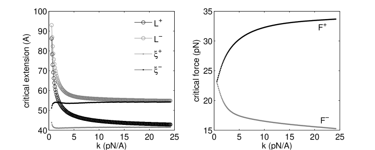
Figure 14: Dependence of the instability of the $F$-$L$ isotherms on the cantilever spring constant $k$ for the [3]rotaxane. The right panel shows the critical values of the force as a function of $k$. Here $F^{+}$ and $F^{-}$ correspond to the values of the force when the $F$-$L$ curves exhibit a maximum and minimum, respectively. The left panel shows the extension lengths $L^{\pm}$ that enclose the unstable region in the $F$-$L$ isotherms, as well as the average end-to-end distance at the critical points $\xi^{\pm}$.

Note that the instability properties of the $F$-$L$ isotherms depend intricately on the cantilever spring constant employed. This dependence is succinctly conveyed in Fig. 14 which shows the values of the extension and the average force at the critical points in the $F$-$L$ isotherms. In the figure, $F^{+}$ and $L^{+}$ (or $F^{-}$ and $L^{-}$) denote the values of the force and the cantilever extension when the $F$-$L$ curve exhibits a maximum (or minimum). These values enclose the unstable region in the $F$-$L$ isotherm. In turn, $\xi^{\pm}$ is the average end-to-end distance at the critical points which is approximately independent of $k$ except for very small $k$. The critical forces $F^{+}$ and $F^{-}$ show a smooth and strong dependence on the cantilever spring constant. For large $k$ the system persistently shows a region of instability in the isotherms. However, as the cantilever spring is made softer, $F^{+}$ and $F^{-}$ approach each other and for small $k$ the mechanical instability in the $F$-$L$ isotherms is no longer present.

III.2.3 Disappearance of the mechanical instability in the soft spring limit

The disappearance of the instability regions in the $F$-$L$ measurements when the system is pulled with a soft cantilever is a general feature of the extension of any molecular system provided that no covalent bond breaking occurs during the process. To see this, consider the soft-spring approximation of the configurational partition function of the system plus cantilever [Eq. (26)]:

$$\frac{Z(L)}{Z_{0}}\approx\frac{\exp(-\beta kL^{2}/2)}{Z_{0}}\int\mathrm{d}\xi\exp[-\beta\phi(\xi)]\exp(\beta kL\xi)=\exp(-\beta kL^{2}/2)\langle\exp(\beta kL\xi)\rangle,$$ (29)

where the notation $\langle f\rangle$ stands for the unbiased (cantilever-free) average of $f$. In writing Eq. (29) we have supposed that in the region of relevant $\xi$ (in which the integrand is non-negligible) $k\xi^{2}/V_{L}(\xi)\ll 1$ and, hence, that the cantilever potential is well approximated by $V_{L}(\xi)\approx\frac{kL^{2}}{2}-kL\xi$. This approximation is valid provided that that no bond breaking is induced during pulling and permits the introduction of a cumulant expansion Kubo (1962) in the configurational partition function. Specifically, the average $\langle\exp(\beta kL\xi)\rangle$ can be expressed as:

$$\langle\exp(\beta kL\xi)\rangle=\sum_{n=0}^{\infty}\frac{(\beta kL)^{n}}{n!}\langle\xi^{n}\rangle=\exp\left\{\sum_{n=1}^{\infty}\frac{(\beta kL)^{n}}{n!}\kappa_{n}(\xi)\right\}$$ (30)

where $\kappa_{n}(\xi)$ is the $n$-th order cumulant. In view of Eqs. (28), (29) and (30) the slope of the $F$-$L$ curves can be expressed as:

$$\frac{\partial\langle F\rangle_{L}}{\partial L}=k-\beta k^{2}\sum_{n=0}^{\infty}\frac{(\beta kL)^{n}}{n!}\kappa_{n+2}(\xi).$$ (31)

It then follows that to lowest order in $k$,

$$\frac{\partial\langle F\rangle_{L}}{\partial L}\approx k>0.$$ (32)

That is, no unstable region in the $F$-$L$ curve can arise in the soft-spring limit, irrespective of the specific form of $\phi(\xi)$. Instabilities, however, can arise in higher orders in the expansion. For instance, to second order in $k$ instabilities arise provided that the cantilever spring constant satisfies:

$$k>\frac{1}{\beta\kappa_{2}(\xi)},$$ (33)

where $\kappa_{2}(\xi)=\langle\xi^{2}\rangle-\langle\xi\rangle^{2}$.

III.2.4 Emergence of the mechanical instability in the stiff spring limit

A mechanically unstable region in the $F$-$L$ curves can only develop if the PMF of the unbiased molecule by itself has a region of concavity. To understand how this result arises consider the configurational partition function of the molecule plus cantilever at extension $L$ [Eq. (26)] for large $k$. In this regime, most contributions to the integral will come from the region where $\xi=L$. Consequently, $\exp[-\beta\phi(\xi)]$ can be expanded around this point to give:

$$\exp[-\beta\phi(\xi)]=\exp[-\beta\phi(L)]\left[1-\beta A_{1}(L)(\xi-L)-\frac{\beta}{2}A_{2}(L)(\xi-L)^{2}+\cdots\right],$$ (34)

where

$$\begin{split}A_{1}(L)&=\frac{\partial\phi(L)}{\partial L},\\ A_{2}(L)&=\frac{\partial^{2}\phi(L)}{\partial L^{2}}-\beta\left(\frac{\partial\phi(L)}{\partial L}\right)^{2}.\end{split}$$ (35)

Here, the notation is such that $\frac{\partial\phi(L)}{\partial L}=\left.\frac{\partial\phi(\xi)}{\partial\xi}\right|_{\xi=L}$. Introducing Eq. (34) into Eq. (26), integrating explicitly the different terms, and performing an expansion around $1/k=0$ one obtains:

$$Z(L)=\sqrt{\frac{2\pi}{k\beta}}\exp[-\beta\phi(L)]\left[1-\frac{1}{2k}A_{2}(L)+\mathcal{O}(1/k^{2})\right].$$ (36)

Using Eq. (28), the derivative of the force can be obtained from this approximation to the partition function. To lowest order in $1/k$ it is given by:

$$\frac{\partial\langle F\rangle_{L}}{\partial L}=\frac{\partial^{2}\phi(L)}{\partial L^{2}}+\frac{1}{2\beta k}\frac{\partial^{2}A_{2}(L)}{\partial L^{2}}+\mathcal{O}(1/k^{2}),$$ (37)

from which it follows that, to zeroth order in $1/k$,

$$\frac{\partial\langle F\rangle_{L}}{\partial L}=\frac{\partial^{2}\phi(L)}{\partial L^{2}}+\mathcal{O}(1/k).$$ (38)

That is, an unstable region in the force vs. extension requires a region of concavity in the PMF.

III.2.5 Relation between force fluctuations and mechanical stability

The mechanical stability properties observed during the AFM pulling experiments are intimately related to the fluctuations in the force measurements. To see this, note that the average slope of the $F$-$L$ curves can be expressed in terms of the fluctuations in the force:

$$\frac{\partial\langle F\rangle_{L}}{\partial L}=\left\langle\frac{\partial^{2}V_{L}(\xi)}{\partial L^{2}}\right\rangle_{L}-\beta[\langle F^{2}\rangle_{L}-\langle F\rangle_{L}^{2}]=k-\beta[\langle F^{2}\rangle_{L}-\langle F\rangle_{L}^{2}],$$ (39)

where we have employed Eq. (28). The sign of $\frac{\partial\langle F\rangle_{L}}{\partial L}$ determines the mechanical stability during the extension and hence Eq. (39) relates the thermal fluctuations in the force measurements with the stability properties of the $F$-$L$ curves. Specifically, for the stable branches for which $\frac{\partial\langle F\rangle_{L}}{\partial L}>0$ the force fluctuations satisfy

$$\langle F^{2}\rangle_{L}-\langle F\rangle_{L}^{2}<\frac{k}{\beta}.$$ (40a)

In turn, at the critical points where the derivative changes sign the force fluctuations satisfy a strong constraint:

$$\langle F^{2}\rangle_{L}-\langle F\rangle_{L}^{2}=\frac{k}{\beta}.$$ (40b)

Last, in the unstable branches the force fluctuations are larger than in the stable branches and satisfy the inequality

$$\langle F^{2}\rangle_{L}-\langle F\rangle_{L}^{2}>\frac{k}{\beta}.$$ (40c)

These inequalities can be employed to determine critical points in the force by measuring the fluctuations even in situations where the fluctuations mask the presence of critical points.

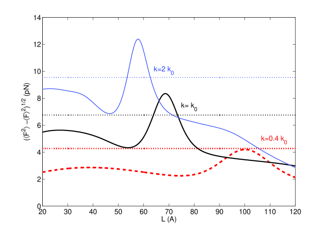
Figure 15: Standard deviation in the force measurements $\sigma_{F}=\sqrt{\langle F^{2}\rangle_{L}-\langle F\rangle_{L}^{2}}$ as a function of $L$ for three different cantilever spring constants $k$ during the pulling of the [3]rotaxane. In each case, the dotted line indicates the value of $\sqrt{k/\beta}$ which sets the limit between the stable and unstable branches in the extension, see Eq. (40).

Figure 15 illustrates these general observations in the specific case of the pulling of [3]rotaxane. As shown, for $k=k_{0}$ and $k=2k_{0}$ there is a region where the force fluctuations become larger than $k/\beta$ and, consequently, unstable behavior in $F$-$L$ develops. For $k=0.4k_{0}$ or less the fluctuations in the force are never large enough to satisfy Eq. (40c) and no critical points in the $F$-$L$ develop, as can be confirmed in Fig. 14.

III.2.6 Origin of the blinking in the force measurements

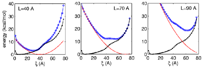
Figure 16: Effective potential $U_{L}(\xi)=\phi(\xi)+V_{L}(\xi)$ for the molecule plus cantilever for different values of the extension $L$. In the panels, the open circles correspond to $U_{L}(\xi)$, the full circles to the PMF $\phi(\xi)$, and the solid lines to the cantilever potential $V_{L}(\xi)$. The cantilever spring constant employed is the same as the one used in the pulling simulations presented in Sec. III.1. Note the bistability in the effective potential for $L=70$ Å.

The observation of force measurements that blink between a high-force and a low force regime (recall Fig. 7) requires the composite system to be bistable along the end-to-end distance for some $L$, i.e. the effective potential $U_{L}(\xi)$ [Eq. (27)] must have a double minimum. Since the PMF of the molecule by itself is not bistable along $\xi$ (see Fig. 9), the bistability must be introduced by the cantilever potential. Figure 16 shows $U_{L}(\xi)$ for selected $L$ for the [3]rotaxane. For $L$ in the stable regions of the free energy ($L=40$ Å  and $L=90$ Å) the effective potential exhibits a single minimum along the $\xi$ coordinate. However, for $L=70$ Å a bistability in the potential develops. The secondary minimum is the cause for the blinking in the force measurements observed at this $L$ (cf. Fig. 7). Further, the relative energy between the two induced minima around the transition region can be manipulated by varying $L$.

What are the minimum requirements for the emergence of bistability along $\xi$? A necessary condition is that the effective potential $U_{L}(\xi)$ is concave for some region along $\xi$, that is:

$$\frac{\partial^{2}U_{L}(\xi)}{\partial\xi^{2}}=\frac{\partial^{2}\phi(\xi)}{\partial\xi^{2}}+k<0.$$ (41)

For Eq. (41) to be satisfied it is required that both: (i) the PMF of the isolated molecule has a region of concavity where $\frac{\partial^{2}\phi(\xi)}{\partial\xi^{2}}<0$, and (ii) the cantilever employed is sufficiently soft such that

$$k<-\text{min}\left(\frac{\partial^{2}\phi(\xi)}{\partial\xi^{2}}\right),$$ (42)

for some $\xi$. Equation (42) imposes an upper bound on $k>0$ for bistability to be observable. If $k$ is stiff the inequality would be violated for all $\xi$ and bistability would not be manifest. Note, however, that there is no lower bound for $k$ that prevents bistability along $\xi$. This is in stark contrast with the behavior of the mechanical instabilities which disappear in the soft-spring limit and persist when stiff springs are employed (see Secs. III.2.2-III.2.5).

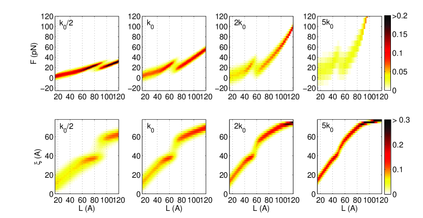
Figure 17: The upper panels show the probability density distribution of the force measurements $p_{L}(F)=\langle\delta[F-F(\boldsymbol{r},L)]\rangle_{L}$ (in pN^-1) during the extension of the [3]rotaxane using cantilevers of varying stiffness. The force function $F(\boldsymbol{r},L)$ is defined by Eq. (3). The lower panels show the associated spatial probability density distributions $p_{L}(\xi)$ (in Å^-1) [Eq. (10)] for the [3]rotaxane plus cantilever. The color code is given in the far right. The spring constants are expressed in terms of $k_{0}=1.1$ pN/Å, the value employed in the pulling simulations presented in Sec. III.1. Note how bistability along $\xi$, and hence blinks in the force measurements, arises for soft cantilevers and decays for stiff ones in accordance with Eq. (42)

Figure 17 illustrates these general observations during the pulling of the [3]rotaxane. Specifically, the figure shows, for cantilevers of varying stiffness, the probability density of observing the value $F$ in the force measurements $p_{L}(F)$ (upper panels) and the associated probability density $p_{L}(\xi)$ that the molecule adopts the extension $\xi$ (lower panels) when the cantilever is fixed at $L$. For soft springs the system satisfies inequality (42) for a range of $L$ values and there is a clear bistability in both probability distributions. As $k$ is increased this bistability becomes less prominent and for $k=5k_{0}$ is no longer observed.

III.2.7 Final remarks

What then should be the picture of the pulling? Clearly, a picture like the one shown in Fig. 12, although appropriate to describe the phenomenology observed in Sec. III.1 around the transition region (and the basis of an influential model of molecular extensibility Rief et al. (1998)), is not accurate since the molecule itself does not show a double well structure along $\xi$ in the free energy. Note, however, that the molecular free energy is inherently bistable along some natural unfolding pathway. If one were able to determine such a pathway, a picture reminiscent to the one shown in Fig. 12 would emerge. However, such natural unfolding pathway is not necessarily accessible during the pulling experiment.

The analogy between first-order phase transition and the isometric single-molecule pulling experiments, even when suggestive, is limited by the fact that the qualitative features observed during pulling strongly depend on the cantilever constant employed. This is because the properties that are measured are those of the combined cantilever plus molecule system. However, as previously noted Kreuzer and Payne (2001), in the stiff spring limit the measured $F$-$L$ curves resemble those which would be obtained from a calculation in the Helmholtz ensemble of the isolated molecule. In this limit, the instability behavior in the force vs. extension will only be due to molecular properties [recall Eq. (38)], and the associated bistability is that observed along the radius of gyration when $\xi$ is fixed in the concave region of the PMF (Fig. 10). It is in this limit that the phenomenology observed during the isometric single-molecule pulling is closest to a first-order phase transition. Experimentally, this limit is impractical since employing a stiff spring reduces the sensitivity in the force measurements.

IV Conclusions

In this contribution we have simulated the equilibrium isometric AFM pulling of a series of donor-acceptor oligorotaxanes by means of constant temperature molecular dynamics in a high dielectric medium using MM3 as the force field. For this system, hysteresis and other nonequilibrium effects that may arise during pulling can be overcome by reducing the pulling speed. The resulting equilibrium force vs. extension isotherms show a mechanically unstable region in which the molecule unfolds and, for selected extensions, blinks in the force measurements between a high-force and a low-force regime.

From the force vs. extension data, the Helmholtz free energy profile for the oligorotaxanes along the extension coordinate was reconstructed using the weighted histogram analysis method, and decomposed into energetic and entropic contributions. The simulations reveal an unfolding pathway for the oligorotaxanes, and indicate that the folding is energetically driven but entropically penalized. Even when the energy and entropy contributions to the potential of mean force can vary widely along the extension, these effects largely cancel one another leading to only modest changes in the free energy profile. Further, we have observed that, for the rotaxanes studied, increasing the number of threaded rings stabilizes the folded conformation, making it resilient to unfolding over a wider range of end-to-end distances. As expected, the elastic properties of the extended conformation are not affected by the number of threaded rings.

The potential of mean force of the rotaxanes exhibits only one minimum along the end-to-end distance. It consists of two stable convex regions characterizing the folded and unfolded conformations and a region of concavity where the unfolding occurs. This thermodynamically unstable region arises because the molecule is inherently bistable. The inherent molecular bistability is not resolved along the end-to-end coordinate (cf. Fig. 9) but, at least in the cases considered, it is manifest along the radius of gyration (recall Fig. 10).

Clearly, modifying the nature of the solvent employed during the pulling can have a quantitative effect on the determined free energy profile since the solvent can vary the relative stability of the different molecular conformations encountered along the extension. Nevertheless, except for very good solvents, the qualitative features of the topography of the potential of mean force described above are expected to remain intact. Also, hydrodynamic effects that may appear when considering an explicit solvent (e.g. drag forces acting on the AFM cantilever due to viscous friction with the surrounding solvent Janovjak et al. (2005)) are immaterial for the equilibrium pulling.

In addition, general conditions on the molecule and on the cantilever stiffness required for the emergence of mechanical instability and blinking in the force measurements in isometric pulling experiments have been presented. Specifically, we have shown that for such effects to arise the potential of mean force of the molecule needs to exhibit a region of concavity along the end-to-end distance. Further, the stiffness of the cantilever employed needs to satisfy specific constraints. For the blinks in the force measurements to arise the cantilever spring constant needs to be sufficiently soft so that Eq. (42) is satisfied. In turn, for the mechanical instability to be observable the fluctuations in the force measurements have to be sufficiently large to satisfy Eq. (40c) for some $L$. In practice, this implies that in the stiff-spring limit the mechanical instability can emerge, while in the soft spring limit the mechanical instability decays regardless of the details of the molecular system, provided that no covalent bond-breaking occurs during pulling.

In this light, it becomes apparent that the analogy presented between first-order phase transitions and the mechanical properties observed during the extension is limited by the fact that the observed behavior depends on the cantilever constant employed. The analogy is the closest in the stiff-spring limit where the mechanical properties recorded are those that would have been obtained in the Helmholtz ensemble of the isolated molecule.

.

.

.