Charge asymmetries in $e^{+}e^{-}\rightarrow\ \pi^{+}\ \pi^{-}\gamma$ at the $\phi$ resonance.

Abstract

We consider the forward-backward pion charge asymmetry for the $e^{+}e^{-}\rightarrow\pi^{+}\pi^{-}\gamma$ process. At tree level we consider bremsstrahlung and double resonance contributions. Although the latter contribution is formally sub-leading, it is enhanced at low dipion invariant mass due to $\rho$ resonant effects. We consider also four alternative models to describe the final state radiation at the loop level: Resonance Chiral Perturbation Theory, Unitarized Chiral Perturbation Theory, Kaon Loop Model and Linear Sigma Model. The last three models yield results compatible with experimental data. The Kaon Loop Model requires an energy dependent phase to achieve the agreement.

I Introduction

The nature of low mass scalar mesons nonet is a long-standing puzzle. The $\phi$ radiative decays are expected to provide information about the $f_{0}\left(980\right)$ and $a_{0}\left(980\right)$ scalar mesons. Unfortunately data reported by the KLOE collaboration on the $\phi$ decays to $f_{0}\gamma$ KLOEf0 and $a_{0}\gamma$ KLOEa0 – with $\pi^{0}\pi^{0}\gamma$ and $\pi^{0}\eta\gamma$ final states respectively– together with results for the $\phi\rightarrow\pi^{+}\pi^{-}\gamma$ process, including the $f_{0}\gamma$ as intermediate state KLOE , are not conclusive. In the latter work, results on the forward-backward asymmetry as a function of the $\pi^{+}\pi^{-}$ invariant mass are presented. The asymmetry is sensitive to the mechanisms involved in the final state radiation kuhn01 and it provides information on the pion form factor PSV . Related work on the reaction $e^{+}e^{-}\rightarrow\ \pi^{+}\ \pi^{-}\gamma$ has been done aiming to elucidate the partonic structure of pions pire .

The asymmetry requires a non vanishing interference between initial (ISR) and final (FSR) state radiation, the latter being strongly model dependent kuhn02 . The invariant amplitude for the $e^{+}e^{-}\rightarrow\pi^{+}\pi^{-}\gamma$ process can be parameterized in terms of three independent Lorentz structures and thus the model dependence in FSR can be included in three scalar functions $f_{i}$ Giulia . The final state radiation has been calculated in different models. The simplest approximation has been named scalar QED kuhn02 ; kuhn03 and it actually includes the $\rho$ contributions to the pion form factor. The contribution of scalars ($f_{0}(980)$ and $\sigma$) have been also considered using a point-like $\phi f_{0}\gamma$ interaction, in the so called ”no-structure” model kuhn02 ; kuhn03 . Later on, the tree level bremsstrahlung of final pions was calculated Giulia ; PSV ; Giulia2 within Resonance Chiral Perturbation Theory ($R\chi PT$) EGPR . In particular, in Giulia2 sub-leading intermediate vector mesons contributions like $e^{+}e^{-}\rightarrow\phi\rightarrow\rho^{\pm}\pi^{\mp}\rightarrow\pi^{+}\pi^{-}\gamma$, named double resonance contributions, were incorporated.

The aim of this paper is to work out the one loop predictions for $e^{+}e^{-}\rightarrow\pi^{+}\pi^{-}\gamma$ at the $\phi$ resonance using four alternative models, namely $R\chi PT$, Unitarized Chiral Perturbation Theory ($U\chi PT$) OO (containing actually a resumation of loops), Linear Sigma Model $\left(LSM\right)$ Levy ; Simon and the so-called ”kaon-loop” model ($KLM$) LN . In each case we add the tree level contributions from bremsstrahlung of pions and the intermediate double resonance, both proposed in Giulia2 . We report the forward-backward pion charge asymmetry and compare our results with KLOE data.

The paper is organized as follows: Section II includes the general formalism to describe the $e^{+}e^{-}\rightarrow\pi^{+}\pi^{-}\gamma$ process. In section III we derive the scalar functions $f_{i}$ that characterize the $R\chi PT$, $LSM$, $U\chi PT$ and $KLM$ contributions, including the tree level bremsstrahlung and double resonance exchange. In section IV we present the numerical results and compare them with data. Finally, conclusions are given in section V.

II General formalism

We are interested in the process

$$e^{-}\left(p_{1}\right)e^{+}\left(p_{2}\right)\rightarrow\pi^{+}\left(p_{+}\right)\pi^{-}\left(p_{-}\right)\gamma\left(k,\epsilon\right).$$ (1)

For completeness, in order to introduce our notation and conventions, in this section we include the basic equations used to describe the process. To this end, we follow the formalism developed in Ref.Giulia . The invariant amplitude $M$ includes the initial state radiation $M_{ISR}$, and final state radiation $M_{FSR}$, i.e. $M=M_{ISR}+M_{FSR}$, with

$$M_{ISR} =-\frac{e}{q^{2}}L^{\mu\nu}\epsilon_{\nu}^{\ast}l_{\mu}F_{\pi}\left(q^{2}\right),\text{ \ \ }$$ (2)

$$\text{\ \ }M_{FSR} =\frac{e^{2}}{s}J_{\mu}M_{F}^{\mu\nu}\epsilon_{\nu}^{\ast},$$ (3)

where $F_{\pi}\left(q^{2}\right)$ denotes the pion electromagnetic form factor, $\epsilon_{\nu}$ is the photon polarization vector and the tensor $M_{F}^{\mu\nu}$ describes the photon radiation from the final state. The lepton currents are given by

$$L^{\mu\nu} =e^{2}\overline{u}_{s_{2}}\left(-p_{2}\right)\times\left[\gamma^{\nu}\frac{\left(-\not p_{2}+\not k+m_{e}\right)}{t_{2}}\gamma^{\mu}+\gamma^{\mu}\frac{\left(\not p_{1}-\not k+m_{e}\right)}{t_{1}}\gamma^{\nu}\right]\times u_{s_{1}}\left(p_{1}\right),$$ (4)

$$J_{\mu} =e\overline{u}_{s_{2}}\left(-p_{2}\right)\gamma_{\mu}u_{s_{1}}\left(p_{1}\right).$$ (5)

The electron and positron spinors are $u_{s_{1}}\left(p_{1}\right)$ and $\overline{u}_{s_{2}}\left(-p_{2}\right)$ respectively. In terms of the external particles’ four-momenta, the following variables are introduced $Q=p_{1}+p_{2},q=p_{+}+p_{-}$,$l=p_{+}-p_{-}$ and five independent Lorentz scalars are defined

$$s \equiv Q^{2}=2p_{1}\cdot p_{2},$$

$$t_{1} \equiv\left(p_{1}-k\right)^{2}=-2p_{1}\cdot k,$$

$$t_{2} \equiv\left(p_{2}-k\right)^{2}=-2p_{2}\cdot k,$$ (6)

$$u_{1} \equiv l\cdot p_{1},u_{2}\equiv l\cdot p_{2},$$

where the electron mass has been neglected. The differential cross section is

$$d\sigma=\frac{1}{2s\left(2\pi\right)^{5}}\int\delta^{4}\left(p_{1}+p_{2}-p_{-}-p_{+}-k\right)\times\frac{d^{3}p_{+}}{2E_{+}}\frac{d^{3}p_{-}}{2E_{-}}\frac{d^{3}k}{2\omega}\overline{\left|M\right|^{2}},$$ (7)

with $p_{+}=\left(E_{+},\mathbf{p}_{+}\right),p_{-}=\left(E_{-},\mathbf{p}_{-}\right)$, $k=\left(\omega=\left|k\right|,\mathbf{k}\right)$ and $\overline{\left|M\right|^{2}}$ is the squared invariant amplitude, averaged over initial lepton polarizations . The most general form of the FSR tensor $M_{F}^{\mu\nu}$ is Giulia

$$M_{F}^{\mu\nu}=f_{1}\tau_{1}^{\mu\nu}+f_{2}\tau_{2}^{\mu\nu}+f_{3}\tau_{3}^{\mu\nu},$$ (8)

where the $\tau_{i}^{\mu\nu}$ are three independent gauge invariant tensors which are dictated by parity, charge conjugation, crossing symmetry and gauge invariance

$$\tau_{1}^{\mu\nu} =k^{\mu}Q^{\nu}-g^{\mu\nu}k\cdot Q,$$

$$\tau_{2}^{\mu\nu} =k\cdot l\left(l^{\mu}Q^{\nu}-g^{\mu\nu}k\cdot l\right)+l^{\nu}\left(k^{\mu}k\cdot l-l^{\mu}k\cdot Q\right),$$ (9)

$$\tau_{3}^{\mu\nu} =Q^{2}\left(g^{\mu\nu}k\cdot l-k^{\mu}l^{\nu}\right)+Q^{\mu}\left(l^{\nu}k\cdot Q-Q^{\nu}k\cdot l\right).$$

The scalar functions $f_{i}\equiv f_{i}\left(Q^{2},k\cdot Q,k\cdot l\right)$ are either even $\left(f_{1,2}\right)$ or odd $\left(f_{3}\right)$ under the change of sign of the argument $k\cdot l$. Our first task will be to determine these scalar functions $f_{i}$ for $R\chi PT$, $U\chi PT$, $LSM$ and $KLM$ in order to add it later to the tree level bremsstrahlung and double resonance exchange Giulia2 .

The pair of pions produced in (1) differ in charge conjugation, depending if the photon is emitted from the initial or from the final state, while the former is odd under charge conjugation the latter is even. So, any interference between the two amplitudes is odd under charge conjugation and gives rise to a charge asymmetry. The forward-backward charge asymmetry is defined as

$$A=\frac{N(\theta_{\pi^{+}}>90^{\circ})-N(\theta_{\pi^{+}}<90^{\circ})}{N(\theta_{\pi^{+}}>90^{\circ})+N(\theta_{\pi^{+}}<90^{\circ})},$$ (10)

where $\theta_{\pi^{+}}$ is the $\pi^{+}$ polar angle, which is measured with respect to the incident electron momentum. It should be clear that the asymmetry depends strongly on the experimental conditions, in particular on the cutoff polar angle and the minimal photon energy that can be measured.

III FSR Models

III.1 Bremsstrahlung

Before discussing the $\phi$ decay models at the loop level, we first consider the bremsstrahlung of the final pions. The corresponding Feynman diagrams are shown in Fig. (1) and the amplitude was calculated in Giulia2 . The functions $f_{i}$ for this contribution are given by equations (11) to (20) in Giulia2 .

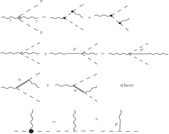
Figure 1: Feynman diagrams for the bremsstrahlung, $a$ corresponds to $a_{1}(1260)$

III.2 Double resonance contribution

The double resonance contribution $e^{+}e^{-}\rightarrow\phi\rightarrow\rho^{\pm}\pi^{\mp}\rightarrow\pi^{+}\pi^{-}\gamma$ is described by the diagrams shown in Fig. (2). This process was calculated in Isidori and used in Giulia2 (equations (26) to (28)), explicitly the $f_{i}$ functions are :

$$f_{1}^{VMD} =-\frac{1}{4\pi\alpha s}\left(\left(-1+\frac{3}{2}x+\frac{4m_{\pi}^{2}}{s}\right)\left(g\left(x_{1}\right)+g\left(x_{2}\right)\right)+\frac{1}{4}\left(x_{1}-x_{2}\right)\left(g\left(x_{1}\right)-g\left(x_{2}\right)\right)\right),$$

$$f_{2}^{VMD} =-\frac{1}{4\pi\alpha s^{2}}\left(g\left(x_{1}\right)+g\left(x_{2}\right)\right),$$ (11)

$$f_{3}^{VMD} =-\frac{1}{4\pi\alpha s^{2}}\left(g\left(x_{1}\right)-g\left(x_{2}\right)\right),$$

where

$$g\left(x\right) =\frac{eg_{\rho\pi}^{\phi}g_{\pi\gamma}^{\rho}}{4F_{\phi}}\frac{m_{\phi}^{2}e^{i\beta_{\rho}}e^{i\beta_{\omega\phi}}}{s-m_{\phi}^{2}+im_{\phi}\Gamma_{\phi}}\frac{s^{2}\Pi_{\rho}^{VMD}}{\left(1-x\right)s-m_{\rho}^{2}+im_{\rho}\Gamma_{\rho}\left(\left(1-x\right)s\right)},$$ (12)

$$x_{1,2} =\frac{2p_{+,-}\cdot Q}{s},\qquad x=2-x_{1}-x_{2,}$$

with the following values for the involved parameters

$$g_{\rho\pi}^{\phi} =0.811\text{ GeV}^{-1},\qquad g_{\pi\gamma}^{\rho}=0.295\text{ GeV}^{-1},$$

$$F_{\phi} =42.5,\qquad\Pi_{\rho}^{VMD}=0.58195,$$

$$\beta_{\rho} =32.996^{\circ},\qquad\beta_{\omega\phi}=163^{\circ}.$$

As we shall see below, this contribution is very important in the description of the charge asymmetries at low dipion invariant mass. It has also been calculated recently Roca:2009zy using the Lagrangian

$$\mathcal{L}=\frac{G}{\sqrt{2}}\epsilon_{\mu\nu\alpha\beta}tr\left(\partial^{\mu}V^{\nu}\partial^{\alpha}V^{\prime\beta}\Phi\right)-4f^{2}egA^{\mu}tr\left(QV_{\mu}\right)+\Theta\phi_{\mu}\omega^{\mu}$$ (13)

where $g=-4.41$, $G=\frac{3g^{2}}{4\pi^{2}f}=0.016$ MeV${}^{-1},$ $Q=diag\left\{2/3,-1/3,-1/3\right\}$ and $e$ is taken positive. The $\phi-\omega$ mixing strength is given by $\widetilde{\varepsilon}=\frac{\Theta}{M_{\phi}^{2}-M_{\omega}^{2}}=0.059\pm 0.004.$ In this scheme we find the $f_{i}$ scalar functions as

$$f_{1} =\alpha\left[\left(l^{2}+k\cdot Q+2k\cdot l\right)D_{\rho}\left(P\right)+\left(l^{2}+k\cdot Q-2k\cdot l\right)D_{\rho}\left(P^{\prime}\right)\right]$$

$$f_{2} =-\alpha\left[D_{\rho}\left(P\right)+D_{\rho}\left(P^{\prime}\right)\right]$$ (14)

$$f_{3} =-\alpha\left[D_{\rho}\left(P\right)-D_{\rho}\left(P^{\prime}\right)\right]$$

where $P=\frac{1}{2}\left(Q+k-l\right)$, $P^{\prime}=\frac{1}{2}\left(Q+k+l\right)$ and $\alpha$ stands for

$$\alpha=-\frac{4f^{4}g^{2}G^{2}\widetilde{\varepsilon}}{9\sqrt{2}M_{\omega}^{2}}D_{\phi}\left(Q\right),$$

which coincides with results in Roca:2009zy whenever $M_{V}=2|g|f.$ This relation is well satisfied numerically and it is possible to show that these functions coincide with (11) up to the phases included in (12) which have a small effect on the asymmetry.

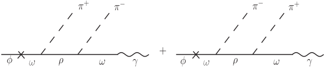
Figure 2: Feynman diagrams for the double resonance contribution

III.3 Contributions from $R\chi PT$ and $U\chi PT$

The amplitude for $e^{+}e^{-}\rightarrow\pi^{+}\pi^{-}\gamma$ at the $\phi$ peak involves the $\gamma\phi\pi^{+}\pi^{-}$ vertex function with all particles on-shell. This vertex function was calculated in the context of $R\chi PT$ and $U\chi PT$ within the analysis of $e^{+}e^{-}\rightarrow\phi\pi\pi$ for an off-shell photon NSOV . The relevant diagrams in $R\chi PT$ EGPR are shown in Fig. (3). These diagrams include kaons in the loops, thus they involve the off-shell $K\overline{K}-\pi\pi$ amplitude. It was shown in NSOV that, to leading order in the chiral expansion, the contribution of diagrams $d,e,f,g$ cancels the off-shell contributions of the $K\overline{K}-\pi\pi$ amplitude, entirely contained in diagrams $a,b,c,h$, so that the calculation reduces to evaluate diagrams $a,b,c,h$ with the $K\overline{K}-\pi\pi$ amplitude on- shell. This procedure yields the $R\chi PT$ result for the $\gamma\phi\pi^{+}\pi^{-}$ vertex function and we would expect it to reproduce experimental results at low dipion invariant mass. However, due to the appearance of the widely discussed light scalar resonance (the $\sigma$ meson), this expansion breaks down in the scalar channel even at the dipion threshold.

The scalar poles can be generated unitarizing the leading order meson-meson scattering amplitudes for definite isospin. Following OO , the unitarized $K^{+}K^{-}-\pi^{+}\pi^{-}$ scattering amplitude is calculated projecting onto the zero spin and isospin channel the leading order meson-meson amplitude and performing a coupled channel analysis involving iterations of all intermediate states in the $s$ channel.

As far as the calculation of the $e^{+}e^{-}\rightarrow\pi^{+}\pi^{-}\gamma$ amplitude is concerned, the scalar poles are incorporated replacing the leading order on-shell $K^{+}K^{-}-\pi^{+}\pi^{-}$ amplitude by the $K^{+}K^{-}-\pi^{+}\pi^{-}$ unitarized amplitude. For details of the calculation we refer the interested reader to NSOV , here we just quote the result for $\phi\rightarrow\pi^{+}\pi^{-}\gamma$. The resulting amplitude for $\phi(Q,\eta^{\alpha\nu})\rightarrow\pi^{+}\left(p_{+}\right)\pi^{-}\left(p_{-}\right)\gamma\left(k,\epsilon^{\mu}\right)$ in $U\chi PT$ is

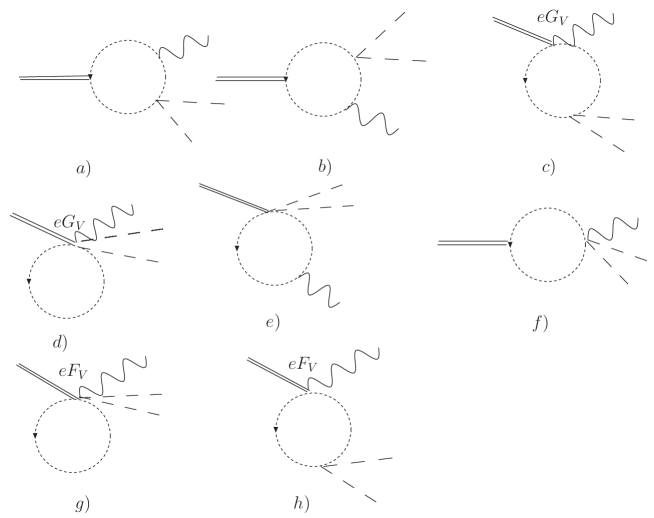
Figure 3: Feynman diagrams for the $\gamma\phi\pi\pi$ vertex function in $R\chi PT$

$$-i\mathcal{M} =\frac{2}{\sqrt{3}}\frac{e}{2\sqrt{2}\pi^{2}m_{K}^{2}f^{2}}\frac{t_{K\pi}^{0}}{\sqrt{3}}\left[G_{V}\left(\widetilde{I}_{P}^{ab}(Q\cdot k\ g_{\mu\nu}-Q_{\mu}k_{\nu})\right)Q_{\alpha}\right.$$

$$-\left.\left(G_{V}-\frac{F_{V}}{2}\right)\frac{m_{K}^{2}}{4}g_{K}(q^{2})g_{\mu\nu}k_{\alpha}\right]\eta^{\alpha\nu}\epsilon^{\mu},$$ (15)

where $q^{2}=(p_{+}+p_{-})^{2}$ and $t_{K\pi}^{0}$ denotes the unitarized isoscalar scalar $K\overline{K}-\pi\pi$ amplitude. The factor $2/\sqrt{3}$ is required to single out the $\pi^{+}\pi^{-}$ contribution in the isoscalar $\pi\pi$ channel. The function $g_{K}(q^{2})$ is given by

$$g_{K}(q^{2})=-1+\log\frac{m_{K}^{2}}{\mu^{2}}+\sigma(q^{2})\log\frac{\sigma(q^{2})+1}{\sigma(q^{2})-1}$$ (16)

with $\sigma(q^{2})=\sqrt{1-\frac{4m_{K}^{2}}{q^{2}}}$. Note that the particular form of this function involves a regularization scheme as well as a subtraction point. We use dimensional regularization and the value $\mu=1.2\,GeV$ which reproduces the $f_{0}$ peak at $980MeV$ in the squared meson-meson amplitudes in the scalar channel OO . The loop integral is given by

$$\widetilde{I}_{P}^{ab} =\frac{1}{2\left(a-b\right)}-\frac{2}{\left(a-b\right)^{2}}\left[f\left(\frac{1}{b}\right)-f\left(\frac{1}{a}\right)\right]+\frac{a}{\left(a-b\right)^{2}}\left[g\left(\frac{1}{b}\right)-g\left(\frac{1}{a}\right)\right],$$ (17)

$$f\left(z\right) =\left\{\begin{array}[c]{c}-\left[\arcsin\left(\frac{1}{2\sqrt{z}}\right)\right]^{2}\text{ \ }z>\frac{1}{4}\\ \frac{1}{4}\left[\ln\left(\frac{n_{+}}{n_{-}}\right)-i\pi\right]^{2}\text{ \ \ \ }z<\frac{1}{4}\end{array}\right.,\text{ \ }g\left(z\right)=\left\{\begin{array}[c]{c}\sqrt{4z-1}\arcsin\left(\frac{1}{2\sqrt{z}}\right)\text{ \ \ \ }z>\frac{1}{4}\\ \frac{1}{2}\sqrt{1-4z}\left(\ln\left|\frac{n_{+}}{n_{-}}\right|-i\pi\right)\text{ \ \ \ }z<\frac{1}{4}\end{array}\right.,$$ (22)

$$\text{ \ \ \ }a =\frac{Q^{2}}{m_{K}^{2}},\text{ }b=\frac{q^{2}}{m_{K}^{2}},\text{ \ }n_{\pm}=\frac{1}{2}\left[1\pm\sqrt{1-4z}\right].$$

Results for $R\chi PT$ are obtained from Eq. (15) by replacing $t_{K\pi}^{0}$ by the leading order on-shell interaction $V_{K\pi}=-\sqrt{3}q^{2}/4f^{2}$. Using the propagator for a vector meson in the tensor formalism we obtain the amplitude for $\gamma^{\ast}(Q,\mu)\rightarrow\pi\pi\gamma(k,\nu)$ via the exchange of the vector meson $\phi$ as

$$-i\mathcal{M}=-\frac{ie^{2}F_{V}\sqrt{2}}{3}\frac{1}{Q^{2}-M_{\phi}^{2}+i\Gamma_{\phi}M_{\phi}}\left[\left(Q^{2}I+J\right)\left(k_{\mu}Q_{\nu}-Q\cdot kg_{\mu\nu}\right)\right]\varepsilon^{\nu},$$ (23)

where

$$I =-\frac{G_{V}}{\sqrt{6}\pi^{2}m_{K}^{2}f^{2}}\frac{t_{K\pi}^{0}}{\sqrt{3}}\widetilde{I}_{P}^{ab},\qquad$$ (24)

$$J =\frac{1}{\sqrt{6}\pi^{2}m_{K}^{2}f^{2}}\frac{t_{K\pi}^{0}}{\sqrt{3}}\left(G_{V}-\frac{F_{V}}{2}\right)\frac{m_{K}^{2}}{4}g_{K}(q^{2}).$$ (25)

In terms of this vertex function we can identify the final state radiation invariant tensor $M_{F}^{\mu\nu}$ (see Eq. 8)

$$M^{\mu\nu}=-ie^{2}(f_{1}\tau_{1}^{\mu\nu}+f_{2}\tau_{2}^{\mu\nu}+f_{3}\tau_{3}^{\mu\nu})=-ie^{2}M_{F}^{\mu\nu}$$ (26)

with

$$f_{1} =-\frac{1}{\sqrt{3}}\frac{F_{V}}{3f^{2}}\frac{1}{Q^{2}-M_{\phi}^{2}+i\Gamma_{\phi}M_{\phi}}\frac{t_{K\pi}^{0}}{\pi^{2}\sqrt{3}}\left(\frac{Q^{2}}{m_{K}^{2}}G_{V}\widetilde{I}_{P}^{ab}-\frac{1}{4}\left(G_{V}-\frac{F_{V}}{2}\right)g_{K}(q^{2})\right),$$ (27)

$$f_{2} =0,$$ (28)

$$f_{3} =0.$$ (29)

Notice that Eq.(27) contains a term with the combination $G_{V}-\frac{F_{V}}{2}$ . This combination is small and it vanishes in the context of Vector Meson Dominance GVFV .

III.4 The phenomenological Kaon Loop Model

In this model the process under consideration proceeds through the chain

$$e^{-}\left(p_{1}\right)e^{+}\left(p_{2}\right)\rightarrow\phi\rightarrow S\left(q\right)\gamma\left(k,\epsilon\right)\rightarrow\pi^{+}\left(p_{+}\right)\pi^{-}\left(p_{-}\right)\gamma\left(k,\epsilon\right),$$ (30)

with $S=f_{0},\sigma$. The corresponding Feynman diagrams of the $\phi$ decay are shown in figure (4). The amplitude is

$$M_{\phi}=\frac{-ie^{2}}{s}A\,e\overline{\,v}\left(p_{2}\right)\gamma_{\mu}u\left(p_{1}\right)\left(Q^{\nu}k^{\mu}-Q\cdot kg^{\mu\nu}\right)\epsilon_{\nu},$$ (31)

where we have defined

$$A=\frac{g_{s}g_{\phi}}{f_{\phi}}\frac{g_{f}}{2\pi^{2}m_{K^{+}}^{2}}\widetilde{I}_{P}^{ab}F_{\phi}\left(s\right)\left[\sum_{S=f,\sigma}\frac{g_{S\pi^{+}\pi^{-}}g_{SK^{+}K^{-}}}{D_{S}\left(q^{2}\right)}\right],$$ (32)

with

$$F_{\phi}\left(s\right)=\frac{m_{\phi}^{2}}{s-m_{\phi}^{2}+i\sqrt{s}\Gamma_{\phi}},\hskip 28.45274ptD_{S}\left(q^{2}\right)=q^{2}-m_{S}^{2}+im_{S}\Gamma_{S},$$ (33)

and $g_{\phi},f_{\phi}$ stand for the $\phi K^{+}K^{-}$ and $\phi\gamma$ couplings respectively (for details concerning the precise definition of these quantities we refer the reader to the appendix of Ref.LN ). The kaon loop function $\widetilde{I}_{P}^{ab}$ is given in (17). It must be mentioned that the $KLM$ does not account for elastic (i.e. non-resonant) $K^{+}K^{-}\rightarrow\pi^{+}\pi^{-}$ scattering of kaons in the loops and the final pions. It has been shown in kuhn02 that this contribution is important in the interference between bremsstrahlung plus double resonance and the $KLM$. This elastic contribution was considered by the introduction of an energy dependent phase in the $KLM$ amplitude. Finally, the scalar functions for this model are obtained by comparing (31) with (3) and (8), in this way we get

$$f_{1} =A,$$

$$f_{2} =0,$$ (34)

$$f_{3} =0.$$

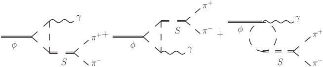
Figure 4: Feynman diagrams for the kaon loop model

III.5 The Linear Sigma Model

The calculation in this approach is similar to the $KLM$, the difference arising from the treatment of the scalars. The Feynman diagrams are shown in figure (5). For the neutral pion case, the amplitude has already been derived in Bramon using the improved chiral loop approach. Thus we can obtain the amplitude we are interested in just by making the following replacement in the $KLM$ amplitude

$$\sum_{S=f,\sigma}\frac{g_{S\pi^{+}\pi^{-}}g_{SK^{+}K^{-}}}{D_{S}\left(q^{2}\right)}\rightarrow\mathcal{A}\left(K^{+}K^{-}\rightarrow\pi^{+}\pi^{-}\right)_{L\sigma M}=\sqrt{2}\mathcal{A}\left(K^{+}K^{-}\rightarrow\pi^{0}\pi^{0}\right)_{L\sigma M}\text{,}$$ (35)

where the amplitude for the meson scattering is given by

$$\mathcal{A}\left(K^{+}K^{-}\rightarrow\pi^{0}\pi^{0}\right)_{L\sigma M} =\frac{m_{\pi}^{2}-q^{2}/2}{2f_{\pi}f_{K}}+\frac{q^{2}-m_{\pi}^{2}}{2f_{\pi}f_{K}}\left[\frac{m_{K}^{2}-m_{\sigma}^{2}}{D_{\sigma}\left(q^{2}\right)}\text{c}_{\phi_{S}}\left(\text{c}_{\phi_{S}}-\sqrt{2}\text{s}_{\phi_{S}}\right)\right.$$

$$+\left.\frac{m_{K}^{2}-m_{f_{0}}^{2}}{D_{f_{0}}\left(q^{2}\right)}\text{s}_{\phi_{S}}\left(\text{s}_{\phi_{S}}+\sqrt{2}\text{c}_{\phi_{S}}\right)\right],$$ (36)

with $f_{K}=1.22f_{\pi}$, $\left(\text{c}_{\phi_{S}},\text{s}_{\phi_{S}}\right)\equiv\left(\cos\phi_{S},\sin\phi_{S}\right)$ and $\phi_{S}$ is the scalar mixing angle in the strange-non-strange basis Simon . The scalar functions for this model can be obtained from (34) by making the replacement in Eq. (35).

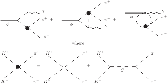
Figure 5: Feynman diagrams for the linear sigma model

IV Numerical results

Numerical results are obtained using a Monte Carlo code where the experimental conditions of the KLOE collaboration are included. Thus, for the $\pi^{+}$ polar angle - defined respect to the electron beam - we considered the range $45^{\circ}<\theta_{\pi^{+}}<135^{\circ}$. As far as the photon is concerned we take $45^{\circ}<\theta_{\gamma}<135^{\circ}$ and assume $E_{\gamma}>10$ MeV KLOE .

Calculations in $U\chi PT$ and $R\chi PT$ involve parameters that have already been fixed from meson phenomenology. We use the following values: $G_{V}=53$ MeV, $F_{V}=154$ MeV, $f_{\pi}=93$ MeV and $\mu=1.2$ GeV OO . Concerning the $KLM$, a summary of the involved parameters is given in Table 1.

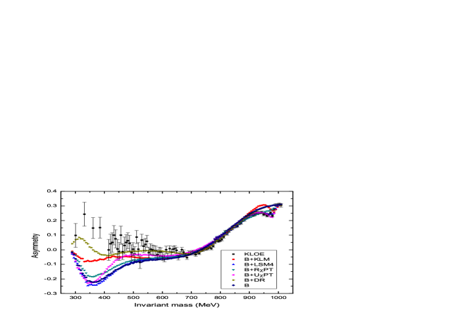
Figure 6: Results for the forward backward asymmetry as predicted by the bremsstrahlung ($B$), bremsstrahlung plus double resonance ($B+DR$) and bremsstrahlung plus loop models for the kaon loop model ($B+KLM$), linear sigma model ($B+LSM4$), resonance chiral perturbation theory ($B+R\chi PT$) and unitarized chiral perturbation theory ($B+U\chi PT$). Data is taken from Refs. KLOE ; tesis .

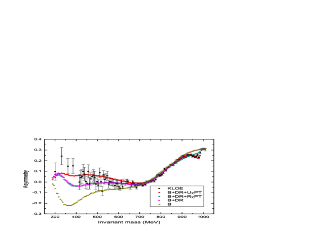
Figure 7: Comparison of the forward backward asymmetry adding to the tree level bremsstrahlung plus double resonance ($B+DR$) the loop level contributions from resonance chiral perturbation theory ($B+DR+R\chi PT$) or unitarized chiral perturbation theory ($B+DR+U\chi PT$) with KLOE data KLOE ; tesis .

Parameter	Value	Reference
$m_{f}$ (MeV)	$980$	PDG
$\Gamma_{f}$ (MeV)	$70$	PDG (Averaged)
$g_{f\pi^{+}\pi^{-}}$ (GeV)	$1.9$	gallegos1
$g_{\sigma\pi^{+}\pi^{-}}$ (GeV)	$2.4$	achasov03
$g_{\phi}$	$4.42$	PDG ; LN
$g_{fK^{+}K^{-}}$ (GeV)	$2.79$	gallegos1
$g_{\sigma K^{+}K^{-}}$ (GeV)	$0.55$	achasov03
$f_{\phi}$	$13.3$	PDG ; LN
$g_{\rho}$	$5.99$	PDG ; LN
$f_{\rho}$	$4.96$	PDG ; LN

Table 1: Constants appearing in the $KLM$ and the numerical values used in this work.

Besides the intrinsic parameters of the scalar mesons, the $LSM$ involves the scalar mixing angle. For the $f_{0}(980)$ we take $m_{f}=980$ MeV, $\Gamma_{f}=70$ MeV, while for the sigma meson we use the values reported in gallegos2 $m_{\sigma}=528$ MeV and $\Gamma_{\sigma}=414$ MeV and for the scalar mixing angle we consider three values: $\phi_{S}=-2^{\circ}$ (LSM2), $-4^{\circ}$ (LSM4) and $-6^{\circ}$ (LSM6).

Our results are shown in Figs. (6,7,8,9,10,11), where aiming to understand the strength of different of the contributions we report partial results. Below we highlight the main findings :

• There are tree level and loop contributions to the $e^{+}e^{-}\rightarrow\pi^{+}\pi^{-}\gamma$ process. The tree level contributions we consider are the bremsstrahlung ($B$) and the double resonance exchange ($DR$) shown in Figs. (1,2). The former is well known to be dominant while the latter is expected to be small due to the $\omega-\phi$ mixing. However this contribution is enhanced at low dipion invariant mass because of $\rho$ resonant effects arising in diagrams of Fig. (2). These resonant effects occur when the energy of the firstly emitted pion is close to $210$ $MeV$, which is kinematically allowed.

• Figure (6) shows the bremsstrahlung ($B$), bremsstrahlung plus double resonance exchange ($B+DR$) and bremsstrahlung plus loop level contributions for the different models considered here ($B+U\chi PT,\,B+R\chi PT,\,B+KLM,\,B+LSM$). bremsstrahlung alone is close to data in the 700-900 MeV region and the remaining contributions do not modify this picture, meaning that they yield negligible contributions in this energy region. However, bremsstrahlung alone does not describe data in the sigma and $f_{0}(980)$ regions. Data is not reproduced at low dipion invariant mass, even if models involving loops are added to the bremsstrahlung contributions. We can see that double resonance contributions turn out to be very important at low dipion invariant mass. Contributions of $B+DR$ are close to data in this energy region in spite of the fact that $DR$ is formally sub-leading due to the $\omega-\phi$ mixing. This is due to the $\rho$ resonant effect mentioned above. In the $f_{0}$ region, data is well described by $B+U\chi PT$ and $B+LSM4$, which contain the $f_{0}$ pole but not by $B,\ B+R\chi PT$ or $B+DR$ where the $f_{0}$ pole is absent. Special mention deserves the $B+KLM$ contributions which in spite of including the $f_{0}$ pole it does not describe data in this region. Below we further discuss this point.

• Figure (7) shows the results obtained from the $U\chi PT$ or the $R\chi PT$ models plus the complete tree level contributions ($B+DR$). Comparison of Figs. (6,7) shows that a constructive interference between $B+DR$ and $U\chi PT$ in the sigma region takes place, and this improves the agreement with data. At high dipion invariant mass the $f_{0}(980)$ pole contained in the $U\chi PT$ amplitude yields the appropriate contributions to achieve agreement with the data. Our results for $B+DR+U\chi PT$ agree with results recently obtained in Roca:2009zy .

• Results for $B+DR+KLM$ are shown in figure (8). Predictions at low dipion invariant mass are close to data but, as mentioned above, the asymmetry in the $f_{0}$ region is not well described. Following Achasov01 ; Achasov02 we studied the effect of an energy dependent phase in the kaon loop amplitude. The authors of Achasov01 ; Achasov02 attribute this phase to the elastic background contributions and they showed this phase to be relevant for the interference between ISR and FSR amplitudes. In the case of charged pions in the final state it was extracted from data as $e^{i\delta_{B}}$ where $\delta_{B}=b\sqrt{q^{2}-4m_{\pi}^{2}}$ with $b=75^{\circ}/GeV$ kuhn02 ; Achasov01 ; Achasov02 . By including this energy dependent phase we obtain good agreement with data in the $f_{0}$ region and data at very low energy is also improved.

• Results for $B+DR+LSM$ are shown in figure (9). The predictions are not sensitive to the scalar mixing angle in the sigma region. In contrast, at high dipion invariant mass, the asymmetry is sensitive to this angle and the best agreement with data is obtained for $\phi_{S}=-4^{\circ}$. This value is close to the one reported in Bramon .

• Figure (10) contains a summary of the best predictions of the models considered in this work. The detail in the 900-1020 MeV region is shown in figure (11).

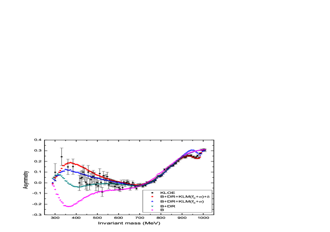
Figure 8: Comparison of KLOE data with the results obtained adding the kaon loop model ($B+DR+KLM(f_{0}+\sigma)$) to the tree level bremsstrahlung plus double resonance exchange ($B+DR$). Points labeled $B+DR+KLM(f_{0}+\sigma)+\delta$ include an energy dependent phase in the kaon loop contributions proposed in Achasov01 ; Achasov02 .

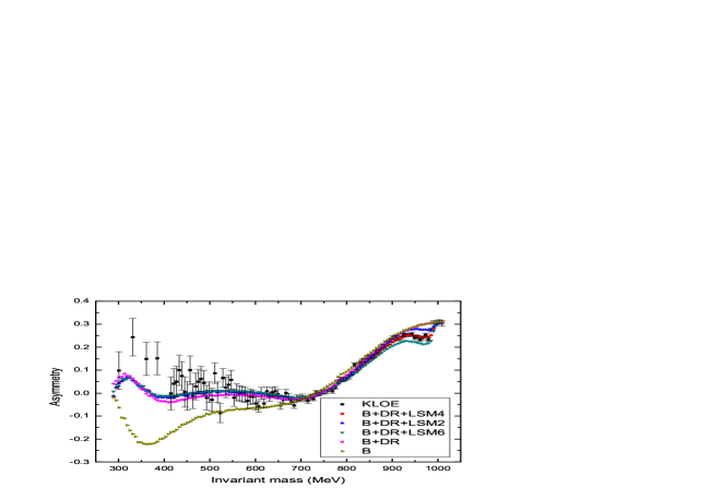
Figure 9: Comparison of KLOE data with results for the forward backward asymmetry as predicted by the $LSM$ using the scalar mixing angles $\phi_{S}=-2^{\circ}$ (LSM2), $-4^{\circ}$ (LSM4) and $-6^{\circ}$ (LSM6).

Finally, we would like to remark that our aim is to explore the compatibility of the considered models with existing data. We find that the models including contributions at the loop level and containing the scalar poles ($U\chi PT$, $LSM$ and $KLM$) are able to reproduce the data. A detailed analysis of the uncertainties in the asymmetry is beyond the scope of this work but it will become compulsory when more precise data at low energies be available so that discrimination between these three models be possible.

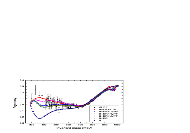
Figure 10: Comparison of KLOE data with predictions of the four models.

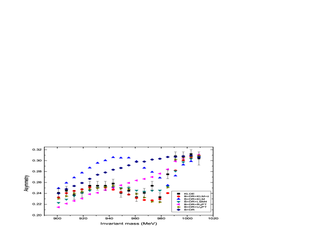
Figure 11: Comparison of KLOE data with predictions of the four models in the 900-1020 MeV region.

V Summary and Conclusions

We consider the theoretical description of the $e^{+}e^{-}\rightarrow\pi^{+}\pi^{-}\gamma$ process. We include tree level contributions (bremsstrahlung and double resonance exchange) as well as loop contributions which are described in terms of four alternative models: Unitary Chiral Perturbation Theory, Resonance Chiral Perturbation Theory, Linear Sigma Model and Kaon Loop Model. We perform a detailed comparison of the model predictions and the KLOE data for the forward-backward charge asymmetry. Our main conclusions are listed below:

• Bremsstrahlung accounts for data in the 700-900 MeV region. Adding double resonance contributions brings predictions close to data at low dipion invariant mass.

• The $R\chi PT$ contributions at loop level are small in the whole kinematic region.

• $U\chi PT$ and $LSM$ yield an appropriate description of data when added to the full tree level contribution (bremsstrahlung plus double resonance exchange).

• Adding $KLM$ to the full tree level contributions yields results that are close to data except in the $f_{0}$ region. Agreement with data in the whole energy range is achieved by including an energy dependent phase proposed in Achasov01 ; Achasov02 in the $KLM$ amplitude.

• The Linear Sigma Model predictions for the asymmetry, at high dipion invariant mass, is highly sensitive to the scalar mixing angle, the value $\phi_{S}=-4^{\circ}$ is favored by data.

• In spite of being suppressed by the $\omega-\phi$ mixing, the double resonance exchange shown in Fig. (2), turns out to be crucial in order to describe the KLOE data in the low dipion invariant mass. This contribution is enhanced due to resonant $\rho$ exchange.

Acknowledgments

Work supported by CONACyT under projects 50471-F and J49178-F. Partial support from DINPO-UG is also acknowledged. We thank J. A. Oller, E. Oset, L. Roca and C. Bini for useful suggestions.

References

- (1) A. Aloisio et al., [KLOE Collaboration], Phys. Lett. B 537, 21 (2002) arXiv:hep-ex/0204013.
- (2) A. Aloisio et al., [KLOE Collaboration], Phys. Lett. B 536, 209 (2002) arXiv:hep-ex/0204012.
- (3) F. Ambrosino et al. [KLOE Collaboration], Phys. Lett. B 634, 148 (2006) arXiv:hep-ex/0511031.
- (4) S. Binner, J. H. Kühn and K. Melnikov, Phys. Lett. B 459, 279 (1999) arXiv:hep-ph/9902399.
- (5) G. Pancheri, O. Shekhovtsova and G. Venanzoni, Phys. Lett. B 642, 342 (2006) arXiv:hep-ph/0605244.
- (6) Z. Lu and I. Schmidt, Phys. Rev. D 73, 094021 (2006) [Erratum-ibid. D 75, 099902 (2007)] [arXiv:hep-ph/0603151]; M. Diehl, T. Gousset, B. Pire and O. Teryaev, Phys. Rev. Lett. 81, 1782 (1998) [arXiv:hep-ph/9805380]; M. Diehl, T. Gousset and B. Pire, Phys. Rev. D 62, 073014 (2000) [arXiv:hep-ph/0003233].
- (7) H. Czyz, A. Grzelinska and H. Kühn, Phys. Lett. B 611, 116 (2005) arXiv:hep-ph/0412239.
- (8) S. Dubinsky, A. Korchin, N. Merenkov, G. Pancheri and O. Shekhovtsova, Eur. Phys. J. C 40, 41 (2005) arXiv:hep-ph/0411113.
- (9) G. Rodrigo, H. Czyz, J. H. Kühn and M. Szopa, Eur. Phys. J. C 24, 71 (2002) arXiv:hep-ph/0112184; H. Czyz, A, Grzelinska, J. H. Kühn and G. Rodrigo, Eur. Phys. J. C 27, 563 (2003) arXiv:hep-ph/0212225.
- (10) G. Pancheri, O. Shekhovtsova and G. Venanzoni, J. Exp. Theor. Phys. 106, 470 (2008) arXiv:0706.3027 [hep-ph].
- (11) G. Ecker, J. Gasser, A. Pich and E. de Rafael, Nucl. Phys. B 321, 311 (1989).
- (12) J. A. Oller and E. Oset, Nucl. Phys. A 620, 438 (1997) [Erratum-ibid. A 652, 407 (1999)]; J. A. Oller, E. Oset and J. R. Pelaez, Phys. Rev. Lett. 80, 3452 (1998) [arXiv:hep-ph/9803242]; J. A. Oller, E. Oset and J. R. Pelaez, Phys. Rev. D 59, 074001 (1999) [Erratum-ibid. D 60, 099906 (1999)] [arXiv:hep-ph/9804209]; J. A. Oller and E. Oset, Phys. Rev. D 60, 074023 (1999) [arXiv:hep-ph/9809337].
- (13) M. Lévy, Nuovo Cim. LIIA 23 (1967); S. Gasiorowicz, D. A. Geffen, Rev. Mod. Phys. 41, 531 (1969); J. Schechter, Y. Ueda, Phys. Rev. D 3, 2874 (1971);
- (14) M. Napsuciale, arXiv:hep-ph/9803396; M. Napsuciale and S. Rodriguez, Int. J. Mod. Phys. A 16, 3011 (2001) [arXiv:hep-ph/0204149].
- (15) J. L. Lucio Martinez and J. Pestieau, Phys. Rev. D 42, 3253 (1990) and J. L. Lucio Martinez and M. Napsuciale, Phys. Lett. B 331, 418 (1994).
- (16) G. Isidori, L. Maiani, M. Nicolaci and S. Pacetti, JHEP 0605:049 (2006) arXiv:hep-ph/0603241.
- (17) L. Roca and E. Oset, Phys. Rev. D 81, 014010 (2010) [arXiv:0911.0994 [hep-ph]].
- (18) M. Napsuciale, E. Oset, K. Sasaki and C. A. Vaquera-Araujo, Phys. Rev. D 76, 074012 (2007) [arXiv:0706.2972 [hep-ph]].
- (19) G. Ecker, J. Gasser, H. Leutwyler, A. Pich and E. de Rafael, Phys. Lett. B 223, 425 (1989).
- (20) A. Bramon, R. Escribano, J. L. Lucio M., M. Napsuciale, G. Pancheri, Eur. Phys. J. C 26, 253 (2002) arXiv:hep-ph/0204339.
- (21) P. Beltrame, Ph.D. Thesis (2009), http://digbib.ubka.uni-karlsruhe.de/documents/711883.
- (22) C. Amsler et al., Phys. Lett. B 667, 1 (2008).
- (23) R. Escribano, A. Gallegos, J. L. Lucio M, G. Moreno and J. Pestieau, Eur. Phys. J. C 28, 107 (2003) arXiv:hep-ph/0204338.
- (24) N. N. Achasov and A. V. Kiselev, Phys. Rev. D 73, 054029 (2006) [Erratum-ibid. D 74,059902 (2006)] [arXiv:hep-ph/0512047].
- (25) A. Gallegos, J. L. Lucio M and J. Pestieau, Phys. Rev. D 69, 074033 (2004) arXiv:hep-ph/0311133.
- (26) N. N. Achasov and V. V. Gubin, Phys. Rev. D 56, 4084 (1997) arXiv:hep-ph/9703367; N. N. Achasov and V. V. Gubin, Phys. Rev. D 57, 1987 (1998) arXiv:hep-ph/9706363.
- (27) N. N. Achasov and V. V. Gubin, Phys. Rev. D 63, 094007 (2001) arXiv:hep-ph/0101024.