Optical conductivity of a metal-insulator transition
for the Anderson-Hubbard model in 3 dimensions away from 1/2 filling

Abstract

The Anderson-Hubbard model is considered to be the least complicated model using lattice fermions with which one can hope to study the physics of transition metal oxides with spatial disorder. We have completed a numerical investigation of this model for three-dimensional simple cubic lattices using a real-space self-consistent Hartree-Fock decoupling approximation for the Hubbard interaction. In this formulation we treat the spatial disorder exactly, and therefore we account for effects arising from localization physics. We have examined the model for electronic densities well away 1/2 filling, thereby avoiding the physics of a Mott insulator. Several recent studies have made clear that the combined effects of electronic interactions and spatial disorder can give rise to a suppression of the electronic density of states, and a subsequent metal-insulator transition can occur. We supplement such studies by calculating the ac conductivity for such systems. Our numerical results show that weak interactions enhance the density of states at the Fermi level and the low-frequency conductivity, there are no local magnetic moments, and the ac conductivity is Drude-like. However, with a large enough disorder strength and larger interactions the density of states at the Fermi level and the low-frequency conductivity are both suppressed, the conductivity becomes non-Drude-like, and these phenomena are accompanied by the presence of local magnetic moments. The low-frequency conductivity changes from a $\sigma-\sigma_{dc}\sim\omega^{1/2}$ behaviour in the metallic phase, to a $\sigma\sim\omega^{2}$ behaviour in the nonmetallic regime. For intermediate disorder at 1/4 electronic filling, a metal-to-insulator transition is predicted to take place at a critical $U/B\approx 0.75$ ($U$ being the Hubbard interaction strength and $B$ the electronic band width). Our numerical results show that the formation of magnetic moments is essential to the suppression of the density of states at the Fermi level, and therefore essential to the metal-insulator transition. At weaker disorder a small lessening of the density of states at the Fermi level occurs, but screening suppresses the spatial disorder and with increasing interactions no metal-insulator transition is found.

I Introduction

Electron-electron interactions are important in understanding the properties of many transition metal oxides.Cox (1992); Imada et al. (1998) Novel ordered phases are found in this class of compounds: e.g., high-$T_{c}$ superconductors, $d$-electron heavy fermions, and quantum magnets. The inclusion of disorder into such materials, and into the models of such systems, adds another level of complexity. In this report we focus on metal-to-insulator transitions that are controlled by the combined effects of both interactions and disorder. In part, this work is part of an effort to understand several experimental results, including the properties of the weakly doped cuprates,Lai and Gooding (1998); Kastner et al. (1998) for which disorder effects are known to be important.

Initially, we were motivated to conduct such theoretical work to better understand this transition in the material LiAl_yTi_2-yO₄.Lambert et al. (1990) The ordered and undoped material LiTi₂O₄ undergoes a transition to a superconducting phaseJohnston (1976); McCallum et al. (1976) around $T_{c}\approx 12~{}K$, and has been proposed to be related to the family of high-$T_{c}$ superconductors.Müller (1996) If such a conjecture is correct, there must be reasonably large electron-electron interactions in this system. The Al-doped system undergoes a metal-insulator transition for $y\approx 0.33$, and recent theoretical work by one of us and co-workers have suggested that (i) the effects of disorder alone cannot lead to such a transitionFazileh et al. (2004); (ii) inclusion of electron-electron interactions in the form of an on-site Hubbard energy can lead to such a transition.Fazileh et al. (2006) This occurs by the suppression of the density of states at the Fermi energy to near zero. The results presented in this report are a natural continuation of such work.

In addition, other systems display such transition. Sarma et al.Sarma et al. (1998) have investigated the electronic structure of LaNi_1-xMn_xO₃. It is known that for a critical concentration of $x_{c}\sim 0.1$ a metal-to-insulator transition is found. The point-contact tunnelling conductance spectra, which provides information on the density of states, show a suppression at the Fermi energy in the form of a downward cusp for both $x=0.05$ and $0.1$. The conductance is found to be proportional to $\sqrt{V}$, where $V$ is the bias voltage. This behaviour was predicted by Altshuler and AronovAltshuler and Aronov (1979), and is similar to the results that we encountered in studies of LiAl_yTi_2-yO₄.Fazileh et al. (2006) Kim et al.Kim et al. (2005) have studied the transport and optical properties of SrTi_1-xRu_xO₃. When $x$ decreases from $1$ to $0$, SrTi_1-xRu_xO₃ evolves from a correlated metal, SrRuO₃ ($x=1$), to a band insulator, SrTiO₃ ($x=0$). Depending on $x$, there are six types of electronic states. The metal-to-insulator transition takes place at $x_{c}\approx 0.5$. As $x$ decreases from one, the concentration of conduction electron decreases, and the effective interaction strength increases.

These systems are very complicated, having several important $d$ orbitals for different conducting sites, and many different interaction, disorder and hopping energy parameters. The theoretical considered below are a minimalist’s approach to such interesting behaviour.

I.1 Anderson-Hubbard Model:

A simplified model that describes interacting electrons moving on a spatially disordered lattice is the so-called Anderson-Hubbard model. Its Hamiltonian is given by

$$\hat{\mathcal{H}}=-t\sum_{\langle ij\rangle,\sigma}(\hat{c}^{{\dagger}}_{i\sigma}\hat{c}_{j\sigma}+\hat{c}^{{\dagger}}_{j\sigma}\hat{c}_{i\sigma})+\sum_{i,\sigma}\varepsilon_{i}~{}\hat{c}^{{\dagger}}_{i\sigma}\hat{c}_{i\sigma}+U\sum_{i}\hat{n}_{i\uparrow}\hat{n}_{i\downarrow}.$$ (1)

Electron annihilation/creation operators for site $j$ and spin $\sigma=\uparrow,\downarrow$ are represented by $\hat{c}_{j\sigma}$ and $\hat{c}^{\dagger}_{j\sigma}$, respectively. The spatially inhomogeneous environment in which the electrons move is accounted for by on-site energies, $\varepsilon_{i}$, which are random. Often, these are selected to be chosen from a uniform distribution, $\varepsilon_{i}\in[-\frac{W}{2},\frac{W}{2}]$, and therefore $W$ is the energy scale characterizing the strength of the disorder. Interactions between electrons are accounted for by the intra-site Hubbard interaction term, characterized by the energy scale $U$. The near-neighbour hopping frequency is denoted by $t$, and all other symbols have their usual meaning. It is hoped that this model can capture some of the essential physics of the metal-insulator transitionsImada et al. (1998) of disordered transition-metal oxides.

The electronic properties of systems described by this model Hamiltonian are indeed complicated, as can be understood from the following reasons. When disorder is sufficiently strong it can lead to the localization of electrons, and favours large electronic occupancies on sites with low on-site energies. Therefore, disorder generates both localization effects and an inhomogeneous distribution of electronic charge. There exists a critical disorder, $(W/t)_{c}$, beyond which all states are localized and the system becomes an Anderson insulator.Grussbach and Schreiber (1995) In a spatially uniform half-filled system, electron-electron interactions also lead to the effective localization of electrons; however, in contrast to disorder, interactions favour single occupancy of electrons on all sites. In general, at a critical interaction, $(U/t)_{c}$, the system undergoes a transition from a metal to a Mott insulator. However, the Mott transition may not take place when the electronic concentration is away from half-filling.

Due to the randomness of the on-site energies, it is usual to address this model using numerical techniques. Also, except for some small clusters that can be solved exactly, large lattices have to be solved with the help of approximate schemes. This difficulty notwithstanding, a small number of “exact” numerical results are available, coming from both exact diagonalization (ED)Paris et al. (2007); Benenti et al. (1999); Berkovits et al. (2001); Kotlyar and Das Sarma (2001); Vasseur and Weinmann (2004); Shinaoka and Imada (2009a) and Monte Carlo (MC)Ulmke and Scalettar (1997); Denteneer et al. (1999); Caldara et al. (2000); Enjalran et al. (2001); Denteneer et al. (2001); Srinivasan et al. (2003); Chakraborty et al. (2007); Chiesa et al. (2008); Paris et al. (2007); Otsuka and Hatsugai (2000) studies. Because of their relevance to our work, we mention one aspect of the results in two of these papers. That is, some ED calculations showed the presence of a suppression of the DOS at the Fermi energy, in both oneShinaoka and Imada (2009a) and twoChiesa et al. (2008) dimensions. These results are consistent with the HF papers mentioned below. Therefore, this provides partial verification of the results based on the HF method, the method used in the remainder of this paper.

I.2 Discussion of Previous HF Results:

The Hartree-Fock (hereafter HF) method is well known, and its application to disordered systems is extensive. The accuracy of the results was recently critiqued by us and coworkers,Chen et al. (2008) where it was shown that provided one allowed for sufficient magnetic degrees of freedom the energies and charge densities of (small) exactly solvable systems agreed well with those obtained from HF. However, since the spin correlations are essentially those of pairs of classical spins of variable directions and lengths, and therefore do not include quantum fluctuations, HF is less successful at capturing the correct spin-spin correlations.

As mentioned, the HF approximation has been applied in many studies of the Anderson-Hubbard and related models. Some examples are (i) a study of a two-dimensional point-defect modelDasgupta and Halley (1993) which represents the acceptors and donors in the high-$T_{c}$ cuprate La_2-xSr_xCuO₄ through determining the magnetic phase diagram, (ii) a proposal of a novel inhomogeneous metallic phase in two dimensionsHeidarian and Trivedi (2004); Trivedi and Heidarian (2005); Trivedi et al. (2005); Kobayashi et al. as a combined effect of disorder and electronic interactions when their strengths are comparable, and (iii) a detailed study of the three-dimensional Anderson-Hubbard model, determining both magnetic and electric phase diagrams at half-filling.Tusch and Logan (1993); Dücker et al. (1999)

In Refs. Tusch and Logan (1993); Dücker et al. (1999), Tusch and Logan have focused on $1/2$-filling and some other fillings lower than $1/8$. At $1/2$-filling with a disorder strength of $W/t=5$, the density of states (hereafter denoted by DOS) shows a suppression for both $U/t=6$ and $9$. Using the inverse participation ratio (IPR) technique, the system is determined to be metallic at $U/t=6$ and insulating at $U/t=9$. The IPR is compared with a threshold mean IPR (obtained in the noninteracting limit) that scales with system size to determine whether the system is metallic or insulating. However, the effect of the interactions on the threshold mean IPR is unknown, as are the effects the unusual statistical distribution of the IPR, the latter having been discussed by Mirlin.Mirlin (2000) In part to circumvent such problems, here we focus on the characterization of the metallicity of a system via its optical conductivity.

In the HF treatment of LiAl_yTi_2-yO₄ by one of us and coworkers,Fazileh et al. (2006) a metal-to-insulator transition, again found from an examination of the behaviour of the IPR, was found. In that work the local magnetic moments were restricted to lie along the $z$-axis, geometrically frustrated corner-sharing tetrahedral lattices were studied, and a quantum site percolation model of disorder was used. Open questions concern whether the suppression of the DOS at the Fermi level depends on the lattice type and the disorder model. To answer these questions, we choose to study three-dimensional simple cubic lattices, which are unfrustrated, and consider a uniform box distribution type of disorder. We also allow local magnetic moments to develop in the $xz$-plane, which increases the spin degree of freedom, believed to be important in some circumstances.Chen et al. (2008)

We also mention the effective-field theory analysis of local moment formation in disordered interacting Fermi liquids by Milovanovic, Sachdev, and Bhatt.Milovanović et al. (1989) The potential importance of such moments in the metal-insulator transition was left as an outstanding question, and will be one of the main aspects addressed in this paper.

I.3 Summary of New Results:

In this paper, we apply the real-space self-consistent HF method to electrons moving on simple cubic lattices at $1/4$-filling, with various strengths of interaction and disorder. Here we report our results from calculations of the DOS and ac conductivity.

When examining systems with a disorder strength of $W/t=6$, we find that the DOS and the low-frequency conductivity are enhanced by a weak interaction ($U/t\leq 3$), and for this range of interactions there are no magnetic moments in the system, and the ac conductivity is Drude-like. With a stronger interaction ($U/t\geq 4$), a suppression of the DOS at the Fermi level and qualitative changes (non-Drude-like) in the low-frequency conductivity are found. We find that concomitant with these changes in behaviour is the appearance of local magnetic moments in the system, although no evidence of magnetic ordering is present. For this disorder strength and electron concentration a metal-to-insulator transition is likely to take place at a critical $U_{c}/t\approx 9$; that is, roughly 3/4 of the noninteracting bandwidth. We have also examined the weaker disorder strength of $W/t=2$, and although one finds a small suppression of the DOS with increasing Hubbard interaction, for no value of $U/t$ do we find a metal-to-insulator transition.

II Real-Space Self-Consistent Hartree-Fock Approximation

For ordered systems, one may transform the Hamiltonian to wave vector space, and then expand the many-particle wave function in a complete set of Bloch wave functions in the corresponding periodic potential. However, in disordered systems there is no translational symmetry, and working in wave vector space does not simplify the problem. Therefore, we will work in real space. In the real-space formulation of HF theory (e.g., see page 349 of Ref. Fazekas (1999)) the disorder is treated exactly, and therefore this approximation allows for us to include in our calculations the effects of localization. In the real-space formulation of HF theory the local Hubbard interaction term is replaced by

$$\hat{n}_{i\uparrow}\hat{n}_{i\downarrow}=\hat{c}^{{\dagger}}_{i\uparrow}\hat{c}_{i\uparrow}\hat{c}^{{\dagger}}_{i\downarrow}\hat{c}_{i\downarrow}$$

$$\approx\langle\hat{n}_{i\downarrow}\rangle\hat{n}_{i\uparrow}+\langle\hat{n}_{i\uparrow}\rangle\hat{n}_{i\downarrow}-\langle\hat{n}_{i\downarrow}\rangle\langle\hat{n}_{i\uparrow}\rangle$$ (2)

$$-\hat{c}^{{\dagger}}_{i\uparrow}\hat{c}_{i\downarrow}\langle\hat{c}^{{\dagger}}_{i\downarrow}\hat{c}_{i\uparrow}\rangle-\hat{c}^{{\dagger}}_{i\downarrow}\hat{c}_{i\uparrow}\langle\hat{c}^{{\dagger}}_{i\uparrow}\hat{c}_{i\downarrow}\rangle+\langle\hat{c}^{{\dagger}}_{i\downarrow}\hat{c}_{i\uparrow}\rangle\langle\hat{c}^{{\dagger}}_{i\uparrow}\hat{c}_{i\downarrow}\rangle.$$

Here, the terms that are proportional to fluctuations about the mean values squared are ignored. Also, we do not consider the expectation values that arise from superconducting correlations.

Substituting Eq. (II) into the Anderson-Hubbard Hamiltonian in Eq. (1), one finds the HF effective Hamiltonian given by

$$\hat{\mathcal{H}}^{\textrm{eff}}=-t\sum_{\langle ij\rangle,\sigma}(\hat{c}^{{\dagger}}_{i\sigma}\hat{c}_{j\sigma}+\hat{c}^{{\dagger}}_{j\sigma}\hat{c}_{i\sigma})$$

$$+\sum_{i,\sigma}\varepsilon^{\textrm{eff}}_{i\sigma}\hat{c}^{{\dagger}}_{i\sigma}\hat{c}_{i\sigma}-U\sum_{i}(h^{-}_{i}\hat{c}^{{\dagger}}_{i\uparrow}\hat{c}_{i\downarrow}+h^{+}_{i}\hat{c}^{{\dagger}}_{i\downarrow}\hat{c}_{i\uparrow}),$$ (3)

where

$$\varepsilon^{\textrm{eff}}_{i\sigma}=\varepsilon_{i}+Un_{i\bar{\sigma}}~{}~{}~{}~{}~{}~{}~{}~{}~{}n_{i\sigma}=\langle\hat{n}_{i\sigma}\rangle$$ (4)

$$h^{+}_{i}=\langle\hat{c}^{{\dagger}}_{i\uparrow}\hat{c}_{i\downarrow}\rangle=\langle\hat{S}^{+}_{i}\rangle~{}~{}~{}~{}~{}h^{-}_{i}=\langle\hat{c}^{{\dagger}}_{i\downarrow}\hat{c}_{i\uparrow}\rangle=\langle\hat{S}^{-}_{i}\rangle$$ (5)

Here, $n_{i\sigma}=\langle\hat{n}_{i\sigma}\rangle$ is the expectation value of the number of electrons with spin $\sigma$ on site $i$; $\varepsilon^{\textrm{eff}}_{i\sigma}$ is the spin dependent effective on-site energy at site $i$, and it is the sum of the original on-site energy plus the Hubbard $U$ times the number of electrons with the opposite spin on that site. Therefore, in the absence of the last term one includes the effects of the Hubbard interaction via an effective shift of the on-site energies. The last term in Eq. (II) does include the $h^{\pm}_{i}$ effective local fields, and these guarantee that the effective Hamiltonian is invariant under rotations in spin space. In the self-consistent formulation of HF theory, one must ensure that the solutions of the effective one-electron Hamiltonian given in Eq. (II) lead to local spin-resolved charge densities and effective local fields that satisfy Eqs. (4,5) when the expectation values are taken with respect to the HF ground state wave function.

II.1 Numerical Approach:

As mentioned above, one is required to solve the effective Hamiltonian self-consistently. In a system with $N_{s}$ sites, one has $4N_{s}$ variational parameters that have to be determined numerically so that the ground-state energy is minimized. (In addition, one includes a chemical potential to fix the electronic density at whatever concentration is desired. In our results below we focus on 1/4 filling.) To solve the effective Hamiltonian self-consistently, one begins with a random initial guess for the $4N_{s}$ parameters that satisfies the constraint of fixing the total number of electrons, and then iterates to self consistency. One needs to repeat the above procedure with many other initial guesses of the variational parameters and below we examine the self-consistent states having the lowest energy HF energies, $E_{\textrm{HF}}$.

After self-consistency is achieved for the HF solutions, we obtain effective single-electron energies, {$E_{n}$}, and the DOS is then given by

$$\textrm{DOS}(E)=\sum_{n}\delta(E-E_{n}).$$ (6)

In our results shown below, we broaden each delta function using a Gaussian function given by

$$f(x)=\frac{1}{d\sqrt{2\pi}}e^{-(x-x_{0})^{2}/2d^{2}},$$ (7)

where $x_{0}$ is where $f(x)$ takes maximum value, and $d$ is the standard deviation (or the broadening width).

To calculate the ac conductivity, one first obtains the imaginary part of the current-current correlation function using the Kubo formula:

$$\textrm{Im}\Lambda_{xx}(\mathbf{q}=0,\omega)=\frac{\pi e^{2}t^{2}}{N_{s}}\sum_{n,m,n\neq m}\Psi^{n,m}(f(\epsilon_{m})-f(\epsilon_{n}))\delta(\omega-(\epsilon_{m}-\epsilon_{n})),$$ (8)

where

$$\Psi^{n,m}=\sum_{\mathbf{i},\mathbf{j},\sigma,\sigma^{\prime}}(\psi^{n}_{\mathbf{i}+\hat{x},\sigma}\psi^{m}_{\mathbf{i},\sigma}\psi^{m}_{\mathbf{j}+\hat{x},\sigma^{\prime}}\psi^{n}_{\mathbf{j},\sigma^{\prime}}-\psi^{n}_{\mathbf{i}+\hat{x},\sigma}\psi^{m}_{\mathbf{i},\sigma}\psi^{m}_{\mathbf{j},\sigma^{\prime}}\psi^{n}_{\mathbf{j}+\hat{x},\sigma^{\prime}}-\psi^{n}_{\mathbf{i},\sigma}\psi^{m}_{\mathbf{i}+\hat{x},\sigma}\psi^{m}_{\mathbf{j}+\hat{x},\sigma^{\prime}}\psi^{n}_{\mathbf{j},\sigma^{\prime}}+\psi^{n}_{\mathbf{i},\sigma}\psi^{m}_{\mathbf{i}+\hat{x},\sigma}\psi^{m}_{\mathbf{j},\sigma^{\prime}}\psi^{n}_{\mathbf{j}+\hat{x},\sigma^{\prime}}).$$ (9)

Then, the real part of the ac conductivity isMahan (2000)

$$\sigma_{1}(\omega)=\frac{\text{Im}\Lambda_{xx}(\mathbf{q}=0,\omega)}{\omega}.$$ (10)

To calculate the ac conductivity numerically, we broaden each delta function in Eq. (8) using a Gaussian function given by Eq. (7). In our results below we state the broadening for each quantity.

III Results

III.1 Disorder Strength:

While the Anderson-Hubbard model is often used to study disordered electronic systems with strong electron-electron interactions, it is not always clear how the parameter space studied for such models relates to real materials, particularly with regards to the strength of the disorder potential. Here we focus on the appropriate range of disorder strengths.

When characterizing the strength of the potential energy it is usual to compare $U$ to the noninteracting bandwidth for electrons moving on an ordered lattice. For a 3d simple cubic lattice that is $B=12t$. Weak interactions correspond to $U/B\ll 1$, intermediate to $U/B\sim 1$, and strong to $U/B\gg 1$. This leads to the question, is it permissible to use the same characterization for the disorder strength?

We have examined the $U=0$ Anderson model (at 1/4 filling - the same as the electronic concentration studied throughout this paper) using a box distribution disorder – all on-site energies between $-W/2$ and $+W/2$ are equally probable. We have then found the ac conductivity of this system for various $W/t$, and here we discuss the results corresponding to $W/t=1,2$ and 6. If one fits our conductivity data to the real conductivity of a Drude model, the latter given by

$$\sigma_{1}(\omega)~{}=\frac{\sigma_{dc}}{1+(\omega\tau)^{2}}~{}~{}~{},$$ (11)

one obtains estimates of the relaxation time and the dc conductivity shown in Table 1. The difference between the $\omega\rightarrow 0$ extrapolations quantifying the dc conductivities are striking, in that for $W/t=1$ we find $\sigma_{dc}\approx 15\pi e^{2}t^{2}$, whereas for $W/t=6$ we find $\sigma_{dc}\approx 0.26\pi e^{2}t^{2}$, implying that the conductivity of these systems differs by almost a factor of 60. Clearly, the noninteracting $W/t=6$ (or equivalently $W/B=1/2$) system corresponds to a “bad metal”. (However, while the $W/t=6$ system is a very poor conductor, for this disorder strength we are not approaching a 1/4-filled Anderson insulator, and, in fact, our calculations and existing dataGrussbach and Schreiber (1995) allow us to determine that $\varepsilon_{F}-\mu_{C}\sim 4t$, with $\mu_{C}$ being the location of the mobility edge.)

Table 1: Conducting properties of noninteracting electrons moving on a 3d simple cubic lattice with a box distribution of disorder of strength $W$, for an electron filling of 1/4. The $\sigma_{dc}$ and $\tau$ are found from fits of the ac conductivity to Eq. (11).

$W/t$	$\sigma_{dc}$ [$\pi e^{2}t^{2}$]	$\tau$ [$t^{-1}$]
1	15.	11.
2	2.3	3.6
6	0.26	0.45

Further justification for this claims follows from a second way of characterizing the “strength” of the disorder, and corresponds to evaluating the elastic mean free path, $\ell_{e}$, in the Born approximation. One findsMott (1990)

$$\frac{\ell_{e}}{a}~{}\approx~{}\frac{4\pi}{z^{2}}~{}\Big{(}\frac{B}{W}\Big{)}^{2}~{}~{}~{},$$ (12)

where $a$ is the lattice constant and $z$ is the coordination number for a particular lattice. Therefore, for $W/t=1$, 2, and 6 one has ${\ell_{e}}/a\approx 50$, 13, and 1.4, respectively. While one does not expect the Born approximation to be accurate quantitatively, especially when it predicts ${\ell_{e}}\approx a$, from these results it follows that for noninteracting electrons moving on a three dimensional simple cubic lattice with $W/B=1/2$ one has a very short mean free path. So, while it might be conventional to refer to a $U/B=1/2$ correlated electronic systems as being intermediate coupling, for a disorder strength of $W/B=1/2$ the system remains metallic but the effect of the disorder potential is indeed very large. As we see in the results below, it is only for such large disorder strengths, which by itself leads to substantial localization effects, that we find a disorder+correlation-driven metal-insulator transition.

(Also, note that in our previous study of lithium titanateFazileh et al. (2006) we employed a quantum site percolation model, which formally corresponds to setting all A site energies to be zero while those on the B sites are infinite - that is, the B sites are removed from the conduction path. With such a large disorder potential (of infinite strength for a binary alloy model of disorder) we did obtain a metal-insulator transition.Fazileh et al. (2006))

III.2 Variation of the Density of States:

As mentioned in the introduction, one of the motivations for this study was to better understand the conditions necessary for the appearance of a suppression in the DOS at the Fermi level. Previous workFazileh et al. (2006); Fazileh (2005) was performed on a lattice appropriate for the description of LiAl$y$Ti_2-yO₄, namely on a corner-sharing tetrahedral lattice. Also, that work was completed using a restricted HF theory: In terms of the above-presented formalism, the effective local fields $h^{\pm}_{i}$ were set to be zero, meaning that the spin degrees of freedom were restricted to develop along the quantization axis ($z$).

All of our results here are for a 3d simple cubic lattice – unlike the corner-sharing tetrahedral lattice, this lattice is bipartite and therefore unfrustrated. In terms of the magnetic degrees of freedom, here we present results from our new HF calculations for two different situations. First, we further restrict the system to be paramagnetic, meaning that we do not allow for the formation of any local moments – this means that $n_{i\uparrow}$ is forced to be equal to $n_{i\downarrow}$. Second, we relax the restriction of the moments being along the $z$-axis, and allow them to form in the $xz$-plane, i.e., $h_{i}^{\pm}$ is nonzero but real.

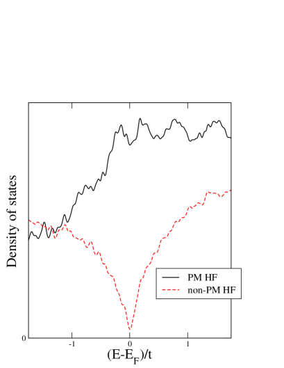
Figure 1: [Colour online] Density of states of a three-dimensional simple cubic lattice of size $18^{3}$ for an electronic filling of $1/4$. The interaction strength is $U/t=11.5$, and the disorder strength is $W/t=6$. The nonparamagnetic HF result (dashed curve) shows a strong suppression of the DOS at the Fermi level, whereas the paramagnetic HF result (solid curve) shows no such suppression. The broadening used corresponds to $d=0.024t$.

Some of our results for the DOS for a three-dimensional simple cubic lattice are shown in Fig. 1. The lattice size is $18^{3}$, and the electronic filling factor is $1/4$. The interaction strength is $U/t=11.5$, where the DOS at the Fermi level has its largest suppression, and the disorder is modelled with a box distribution for a disorder strength of $W/t=6$. The nonparamagnetic HF result shows a strong suppression of the DOS at the Fermi level; however, the paramagnetic HF result shows no suppression at all.

Since we only found a suppression of the DOS with nonparamagnetic HF solutions, both with $h_{i}^{\pm}=0$ (in Ref. Fazileh et al. (2006)) and $h_{i}^{\pm}$ being real, the magnetic moments are essential to the suppression and to the metal-insulator transition (at least within the HF context). The moments found for the real $h_{i}^{\pm}$ HF ground state are strongly noncollinear – e.g., see our discussion in Ref. Chen et al. (2008). Therefore, the restriction of collinear moments employed in Refs. Fazileh et al. (2006) is not important to the suppression. Also, the type of lattice does not matter because the suppression is found both for the frustrated corner-sharing tetrahedral lattices (in Ref. Fazileh et al. (2006)) and for the unfrustrated simple cubic lattices studied in this paper. Also, the type of disorder does not matter, since the suppression is found either with a quantum site percolation model (in Ref. Fazileh et al. (2006)) or with a uniform box distribution type of disorder.

To better quantify the presence of the local moments we have calculated the average magnitude of the moment per electron. We define an Edwards-Anderson-like order parameter

$${\overline{m}}=\frac{1}{N_{e}}\sum_{i=1}^{N_{s}}|\langle\hat{\mathbf{S}}_{i}\rangle|,~{}~{}~{}~{}~{}\hat{\mathbf{S}}_{i}\equiv\frac{1}{2}\hat{c}^{\dagger}_{i\sigma}{\vec{\tau}}_{\sigma\sigma^{\prime}}\hat{c}_{i\sigma^{\prime}}$$ (13)

where $\hat{\mathbf{S}}_{i}$ is the spin operator on site $i$, ${\vec{\tau}}$ are the Pauli matrices, and $N_{e}$ ($N_{s}$) is the number of electrons (lattice sites). The quantity ${\overline{m}}$ is similar to the Edwards-Anderson order parameterEdwards and Anderson (1975) in spin glass theory, which is used to distinguish between glass and nonglass phases,Xue and Lee (1988) but here we use ${\overline{m}}$ as a characterization of local magnetic moment formation.

We have considered many different parameter sets and lattice sites (see discussions below), and our results for ${\overline{m}}$ are shown in Fig. 2. We see that are no local moments in the noninteracting ($U/t=0$) or weakly interacting systems ($U/t\leq 3$) for $W/t~{}=~{}2$ and 6. For the $18^{3}$ lattice and $U/t=3$ and $W/t=6$, ${\overline{m}}$ is only about $0.0045$, and for the $18^{3}$ lattice and $U/t=3$ and $W/t=2$ we find ${\overline{m}}=0.00002$; therefore, this quantity is expected to be zero in the thermodynamic limit. For larger $U/t$ we do find moments, and for a given interaction strength ${\overline{m}}$ increases as one increases the strength of the disorder. In all of the subsequent data that we show having a suppression of the DOS at the Fermi level, and non-Drude-like conductivity, the average magnitude of the local magnetic moments $\overline{m}$ is always nonzero.

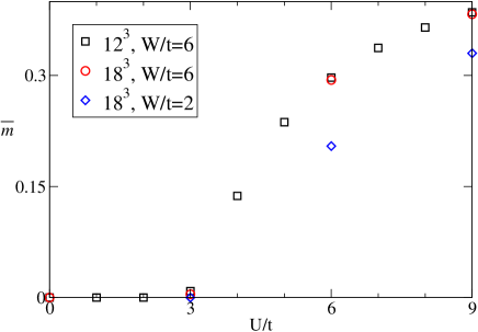
Figure 2: [Colour online] The average magnitude of the magnetic moment per electron (${\overline{m}}$) vs. interaction strength ($U/t$) for a $12^{3}$ lattice with disorder strength $W/t=6$ (squares), and for an $18^{3}$ lattice with $W/t=2$ (diamonds) and $6$ (circles).

Now, we consider the variation of the DOS in more detail. We have calculated the DOS for a $1/4$-filled three-dimensional simple cubic lattice of size $12^{3}$ for various strengths of interaction $U/t=0$, $1$, $2$, …, $8$, $9$, and $11.5$. The on-site energies obey a uniform box distribution, and the disorder strength is $W/t=6$. Results are averaged over $4$ realizations of disorder – a limited study using more realizations of disorder found no qualitative changes when more realizations were employed. The maximum differences for the self-consistency are between $2\times 10^{-5}$ (for $U/t=1$ and $2$) and $1.2\times 10^{-3}$ (for $U/t=11.5$). (Typically, the average differences were at least one order magnitude smaller than the maximum differences.) In Fig. 3, we show the DOS of this system obtained with $d=0.048t$. (The DOS curves are smooth and well separated from one another around the Fermi level, whereas for smaller broadening these curves are bumpy and not well separated, and we therefore choose $d=0.048t$ as the broadening width for the DOS of this system.)

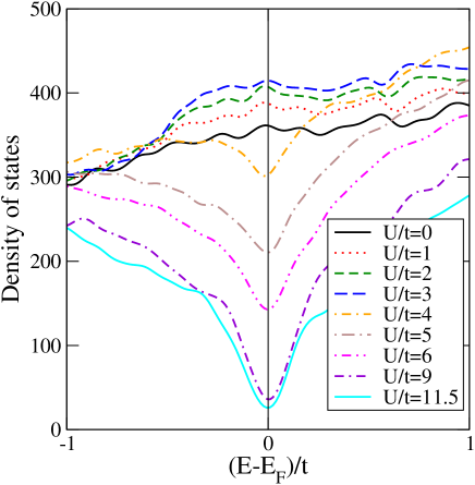
Figure 3: [Colour online] Density of states of the Anderson-Hubbard model on a $1/4$-filled three-dimensional simple cubic lattice of size $12^{3}$ for a disorder strength of $W/t=6$. Results without interactions ($U/t=0$) and with interaction strengths $U/t=1$, $2$, …, $6$, $9$, and $11.5$ are averaged over $4$ realizations of spatial disorder. The vertical line represents the Fermi level. The broadening width is $d=0.048t$.

As shown in Fig. 3, for $U/t=0$ to $3$, each DOS does not show any suppression. In fact, the DOS at the Fermi level is enhanced as the interaction is turned on and then increased. The suppression appears for the first time when $U/t=4$, and the amount of the suppression increases as $U/t$ is increased. We find that the maximum suppression, for 1/4 filling, occurs around $U/t=11.5$, although there is little difference between the DOS for this $U/t$ and other Hubbard interactions close to this strength.

III.3 Behaviour of the Optical Conductivity:

Extracting the low-frequency behaviour of the conductivity is nontrivial, and we briefly outline the numerical approach taken. We have examined the ac conductivity obtained with different values of the Gaussian broadening width $d$ in Eq. (7), and have selected a value for $d$ based on the following: For a three-dimensional simple cubic lattice of size $12^{3}$ with disorder strength $W/t=6$ and interaction strength $U/t=6$, we calculated the ac conductivity with broadening widths $d=0.012t$, $0.03t$, and $0.06t$ (results not shown). Because the broadening width $d$ has a finite value, the contributions of frequencies between $0$ and $d$ makes the imaginary part of the current-current correlation function $\textrm{Im}\Lambda(\mathbf{q}=0,\omega)=\omega\sigma_{1}(\omega)$ nonzero around $\omega=0$. As a result, when calculating $\sigma_{1}(\omega)$ by dividing $\textrm{Im}\Lambda(\mathbf{q}=0,\omega)$ by $\omega$, we obtain diverging $\sigma_{1}(\omega)$ around $\omega=0$. The divergence is simply an artifact of numerical procedure used (a broadening width $d$ that is finite), and is not associated with the physics of the system being investigated. Therefore, we have to cut off the conductivity curves at low frequencies ($\sim d$) where they “turn up”. Recalling that the DOS data of Fig. 3 used $d=0.048t$, we choose $d=0.03t$ as the broadening width for the conductivity because the corresponding conductivity curves are smooth and still retain much of the low-frequency behaviour – simply, we are not forced to discard as much low-frequency data as we would with $d=0.048t$. (As reviewed in the discussion, this low-frequency behaviour is an important quantity to know.)

We now discuss our results, juxtaposing DOS and ac conductivity data for each parameter set. First, we discuss results for studies done on lattices of size $12^{3}$ with a disorder strength of $W/t=6$; an average over $4$ realizations of disorder is used for each data set. We increase the interaction strength $U/t$ from zero up to roughly $12$.

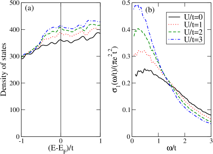
Figure 4: [Colour online] Density of states (a) and ac conductivity (b) for a $1/4$-filled three-dimensional simple cubic lattice of size $12^{3}$ with a disorder strength $W/t=6$ with no interactions ($U/t=0$) and with Hubbard interaction of strengths $U/t=1$, $2$, and $3$. The DOS do not show any suppression at the Fermi level, and in fact increase as the interaction strength $U/t$ increases. The low-frequency conductivity is enhanced as $U/t$ is increased, and the ac conductivity is Drude-like. We have used a broadening corresponding to $d=0.048t$ for the DOS and $d=0.03t$ for the conductivity.

The results for the noninteracting case ($U/t=0$) and for interactions $U/t=1$, $2$, and $3$ are shown in Fig. 4. The solid lines in (a) and (b) represent the DOS and the ac conductivity for the noninteracting electrons, respectively. The ac conductivity has a shape that is typical of a metal, but the low-frequency peak is broad. When we turn on the interaction to $U/t=1$ (dotted lines), we see an enhancement in the DOS at the Fermi level. Concomitantly, the low-frequency ac conductivity also increases from the noninteracting value. These enhancements could be a result of the screening of the disorder by the Hubbard interactions. As the interaction strength $U/t$ increases to $2$ (dashed lines) and $3$ (dash-dotted lines), we find that the DOS at the Fermi level and the low-frequency ac conductivity are both further enhanced. Therefore, for a disorder of $W/t=6$ at 1/4 filling, a weak interaction of $U/t\leq 3$ enhances the low-frequency ac conductivity due to an increase in the DOS at the Fermi level. Recall, from Fig. 2, that for this range of interaction strengths no local moments are formed.

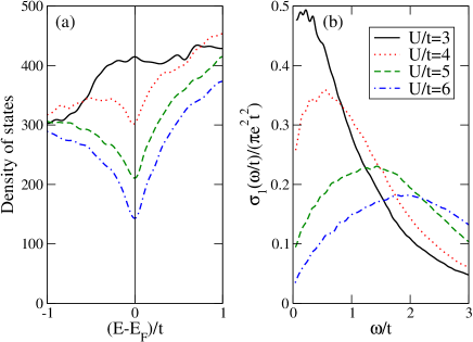
Figure 5: [Colour online] Density of states (a) and ac conductivity (b) for a $1/4$-filled three-dimensional simple cubic lattice of size $12^{3}$ with a disorder strength $W/t=6$ and Hubbard interaction strengths $U/t=3$, $4$, $5$, and $6$. Each of the DOS for $U/t=4$, $5$, and $6$ shows a suppression at the Fermi level, and the amount of the suppression increases as $U/t$ increases. The low-frequency conductivity decreases as $U/t$ increases, and the ac conductivity is no longer Drude-like.

The results for interactions $U/t=3$, $4$, $5$, and $6$ are shown in Fig. 5. A suppression of the DOS at the Fermi level first appears for $U/t=4$, and its value is smaller than that of the noninteracting electrons and that of the $U/t=3$ system. The low-frequency conductivity for $U/t=4$ is also smaller than that of the $U/t=3$ system. As the interaction strength $U/t$ increases to the values of $5$ and $6$, the amount of the suppression of the DOS at the Fermi level increases, and the low-frequency conductivity decreases. Each of the ac conductivity curves still extrapolates to a nonzero value when the frequency $\omega/t\rightarrow 0$. We note that starting from $U/t=5$, the low-frequency conductivity is smaller than that of the noninteracting electrons. More importantly, the ac conductivity for $U/t=4$, $5$, and $6$ is no longer Drude-like. In fact, our conductivity curves are similar to the localization-enhanced Drude theory of Mott and Kaveh,Mott. and Kaveh (1985) and such conductivities have been observed experimentally previously in the metallic phase near the metal-insulator transition in experimental work on conducting polymers.Lee et al. (1993)

We show the results for interaction strengths $U/t=6$, $9$, and $11.5$ in Fig. 6. Compared to $U/t=6$, the DOS at the Fermi level gets further suppressed. However, the amount of the suppression for $U/t=9$ and $11.5$ are not that different. It is very clear that, on the scale of Fig. 6, the dc conductivity for $U/t=9$ and $11.5$ are both zero. The ac conductivity for $U/t=9$ and $11.5$ both increase as $\omega/t$ increases up to the value of $\omega/t\sim 3$.

We fit the ac conductivity for $U/t=6$, $9$, and $11.5$ with power-law relations. For $U/t=6$, the system appears to be metallic, and we fit its ac conductivity using the following equation:

$$\sigma_{1}(\omega)=\pi e^{2}t^{2}(\sigma_{0}+\beta\omega^{\alpha}),$$ (14)

where $\sigma_{0}$, $\beta$, and $\alpha$ are the parameters to be determined. The range of frequency over which we chose to fit the data is $0.04<\omega/t<1.2$ (recall that we used $d=0.03t$ in producing these conductivity curves), and we obtain

$$\sigma_{1}(\omega/t)/(\pi e^{2}t^{2})=(0.002\pm 0.001)$$

$$+(0.145\pm 0.001)(\omega/t)^{0.501\pm 0.007}.$$ (15)

Here, the uncertainties are one standard deviation. We learn from this power-law fit that the dc conductivity for the system with $W/t=U/t=6$ is $\sigma_{0}=0.002\pm 0.001$, which is quite close to but still above zero. Therefore, we expect that the system is a metal. We also see that the exponent of the frequency is $\alpha=0.501\pm 0.007$, which is the exponent ($0.5$) that appears in the ac conductivity of noninteracting electrons with strong disorder, in the metallic regime close to the transition,Kroha (1990) where $\sigma_{1}(\omega)$ near $\omega=0$ goes as $\sigma_{1}(\omega)-\sigma_{0}\sim\sqrt{\omega}$.

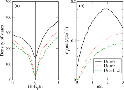
Figure 6: [Colour online] Density of states (a) and ac conductivity (b) for a $1/4$-filled three-dimensional simple cubic lattice of size $12^{3}$ with a disorder strength $W/t=6$ and Hubbard interactions of strength $U/t=6$, $9$, and $11.5$. Each DOS shows a suppression at the Fermi level, and the low-frequency conductivity is also suppressed – both suppressions increase with increasing interactions. The ac conductivity for $U/t=6$ extrapolates to a nonzero dc conductivity as $\omega/t\to 0$, however, the dc conductivity for $U/t=9$ and $11.5$ are both very close to zero.

We fit the ac conductivity for $U/t=9$ and $11.5$ over the ranges of $\omega/t\in[0.074,0.267]$ and $\omega/t\in[0.074,0.330]$, respectively. Setting $\sigma_{0}=0$ we obtain

$$\sigma_{1}(\omega/t)/(\pi e^{2}t^{2})=(0.23\pm 0.01)(\omega/t)^{1.89\pm 0.02}$$ (16)

for $U/t=9$ and

$$\sigma_{1}(\omega/t)/(\pi e^{2}t^{2})=(0.178\pm 0.006)(\omega/t)^{2.05\pm 0.02}$$ (17)

for $U/t=11.5$. These exponents are very close to $2$, and, again, this is the same as the exponent for noninteracting electrons for an even stronger disorder, namely for a disordered system in the insulating phase,Kroha (1990) where $\sigma_{1}(\omega)\sim\omega^{2}$ in the low-frequency regime.

Therefore, the system with $W/t=6$ is metallic for $U/t\leq 6$ and insulating for $U\gtrsim 9$. By examining other $U/t$ around 9 (data not shown) we can identify that the metal-to-insulator transition for this disorder and electronic filling indeed takes place at some critical $(U/t)_{\textrm{cr}}\approx 9$.

It is always desirable to complete studies with larger lattices, where finite-size effects are hopefully less punitive. In our study the benefits of having such data are (i) better energy resolution of the DOS near the Fermi level, and below we make clear the usefulness of such data; and (ii) better resolution of the ac conductivity at low frequencies. Using our computer resources the largest lattice that we have managed to treat, and are able to explore various parameters sets, is an $18^{3}$ lattice with $1/4$-filling. For this lattice with our HF formulation employing real $h_{i}$, it takes about one month to achieve self-consistency in the HF calculations for a single realization of disorder, and due to this enormous amount of time we solve the problem only for one realization of disorder.

For a disorder strength of $W/t=6$ and interaction strengths of $U/t=0$, $3$, $6$, and $9$, we show the resulting DOS in Fig. 7. (Due to the higher number of energy levels per unit frequency we have used 1/2 the broadening width ($d=0.024t$) as we did for the 12³ studies.) We note that the behaviour of the DOS in this larger lattice is very similar to the $12^{3}$ lattice that we have studied earlier.

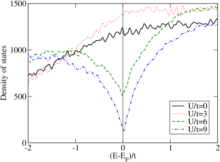
Figure 7: [Colour online] Density of states for the Anderson-Hubbard model on a $1/4$-filled three-dimensional simple cubic lattice of size $18^{3}$. For an intermediate disorder of $W/t=6$, interaction strengths of $U/t=0$, $3$, $6$, and $9$ are considered. The Gaussian broadening width is $d=0.024t$.

The corresponding ac conductivity for the same system is shown in Fig. 8. Note that this data corresponds to a very small Gaussian broadening of only $d=0.01t$, and therefore we can obtain data down to very low frequencies. We clearly see that the data is similar (qualitatively and quantitatively, indicating that our data does not suffer from strong finite-size effects) to that shown earlier for a 12³ lattice. Further, the extrapolation of the conductivity in the zero frequency limit makes clear the nonconducting nature of the $U/t=9$ system.

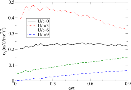
Figure 8: [Colour online] AC conductivity of the Anderson-Hubbard model on a $1/4$-filled three-dimensional simple cubic lattice of size $18^{3}$ for a disorder potential of strength $W/t=6$, for interaction strengths of $U/t=0$, $3$, $6$, and $9$. The Gaussian broadening width is $d=0.01t$.

III.4 System with a weak disorder:

So far, we have studied systems with a disorder strength of $W/t=6$. As mentioned earlier, this corresponds to a noninteracting disordered electronic system with a very low dc conductivity – that is, this corresponds to a “bad metal”. We found a suppression of the DOS at the Fermi level for interaction strengths $U/t\geq 4$. When this happens, we find that the ac conductivity is no longer Drude-like, and for strong enough interactions, $U/t\sim 9$, the system no longer possesses a metallic conductivity. A natural question then arises: For smaller strengths of disorder does one still obtain a metal-insulator transition?

In this subsection we present our results for a weaker disorder corresponding to $W/t=2$. Compared to the noninteracting $W/t=6$ system, the noninteracting $W/t=2$ system has a mean free path and dc conductivity almost an order of magnitude larger.

For such disorder we are forced to use a large lattice because the energies are strongly degenerate in small lattices. In Fig. 9 we show the DOS for an $18^{3}$ simple cubic lattice with interaction strengths $U/t=3$, $6$, $9$, $11.5$, $12$, and $15$.

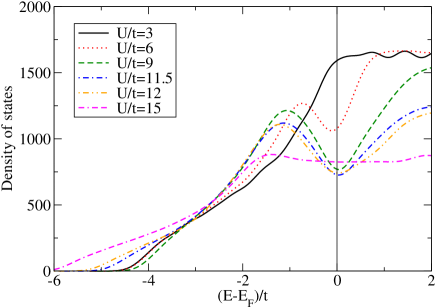
Figure 9: [Colour online] Density of states for a $1/4$-filled three-dimensional simple cubic lattice of size $18^{3}$ with a box distribution type of disorder of strength $W/t=2$ ($4$ realizations of disorder) and Hubbard interaction of strengths $U/t=3$, $6$, $9$, $11.5$, $12$, and $15$.

For this weak disorder strength, the interaction strength of $U/t=3$ does not produce a suppression in the DOS at the Fermi level. However, for $U/t=6$, $9$, $11.5$ and $12$ a suppression in the DOS appears at the Fermi level, and the amount of suppression is deepest at $U/t=11.5$. For $U/t=15$ we find that the suppression has been eliminated.

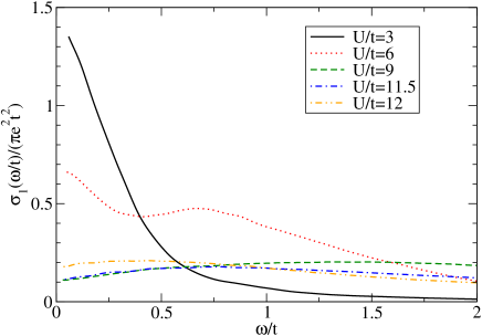
Figure 10: [Colour online] AC conductivity for a $1/4$-filled three-dimensional simple cubic lattice of size $18^{3}$ with a box distribution type of disorder of strength $W/t=2$ ($4$ realizations of disorder) and Hubbard interaction of strengths $U/t=3$, $6$, $9$, $11.5$, and $12$.

In Fig. 10, we show the ac conductivity for the same system with interaction strengths up to $U/t=12$. The conductivity for $U/t=3$ is clearly metallic and Drude like, and extrapolates to roughly $\sigma_{dc}\approx 1.4\pi e^{2}t^{2}$ in the low-frequency limit. This value is roughly half that of noninteracting electrons with the same strength of disorder.

With increasing $U/t$ the conductivity at low frequencies is lowered, with $U/t=9$ and 11.5 having very similar behaviour. However, for $U/t=12$ the conductivity increases near $\omega=0$ – this behaviour persists for even larger Hubbard energies. Therefore, this disorder strength does not lead to a nonmetallic conductivity for any Hubbard energy that we have studied.

To aid in the understanding the above results, namely that for a larger disorder one does obtain a metal-insulator transition, whereas for smaller disorder one does not, we have examined the local charge densities for these parameter sets. In Fig. 11, we show histograms of the local charge density for the $18^{3}$ lattice with disorder strength $W/t=6$ for $U/t=0$ and $9$ (a), and $W/t=2$ for $U/t=0$ and $11.5$ (b).

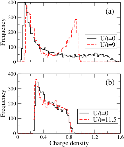
Figure 11: [Colour online] Histograms of the local charge density for the $18^{3}$ lattice. (a) $U/t=0$ and $9$ for a disorder $W/t=6$. (b) $U/t=0$ and $11.5$ for a weak disorder $W/t=2$.

For disorder strength $W/t=6$, when the system is noninteracting the charge density is spread out over a large range, with one large peak close to $n\sim 0.1$. That is, in the absence of interactions and for this seemingly large disorder (see previous discussion) the ground state corresponds to a very small occupation of sites with large on-site energies, with a increasing occupation as the on-site energies decrease. However, when the interaction strength is strong ($U/t=9$), the original peak at the small charge density does not change much, but a large new peak around $n\approx 0.9$ forms. That is, for this disorder the interactions lead to very different charge densities, and correspond to those of an insulating system. The contrasting situation for weak disorder is clear from the figure – the charge distribution is quite similar between the noninteracting ($U/t=0$) and strongly interacting ($U/t=11.5$) systems, and in both cases one has metallic conduction.

We have also plotted the histograms for the effective on-site energies, that is $\varepsilon^{\textrm{eff}}_{i\sigma}$ from Eq. (4) averaged over both spins, since this quantity has been suggested to be important in the understanding of the metallicity of such ground states.Song et al. (2008); Henseler et al. (2008) However, the histograms for $\langle\varepsilon^{\textrm{eff}}_{i\sigma}\rangle_{\sigma}$, for the same parameter sets as those used in Fig. 11, show essentially no difference for these interacting HF ground states, one of which we found to be metallic and one insulating.

IV Discussion

Our numerical analysis of the real-space self-consistent HF treatment of the Anderson-Hubbard model away from 1/2 filling on 3d simple cubic lattices gives rise to three main conclusions, each of which we discuss in relation to previously published theoretical and experimental work.

• At least at 1/4 filling, and thereby well away from 1/2 filling, one requires sufficiently strong disorder to obtain a metal-to-insulator transition.

As preliminary work to our study, we first characterized the consequences of different strengths of disorder for noninteracting electrons. For a disorder strength much less than the noninteracting bandwidth, given by $B=12t$, we find a large dc conductivity, consistent with theoretical predictions of a large mean free path. However. for a disorder strength that is 1/2 of this bandwidth, we find a greatly reduced dc conductivity, and applying Eq. (12), estimate a mean free path of the same order as the lattice constant. Therefore, for the latter disorder strength the effects of the localization of electronic eigenstates is considerable. Note that we have treated the disorder of the Anderson-Hubbard model exactly, and have solved systems having large lattices with as many as 18³ sites, thereby allowing for such localization physics to be present in our HF ground states.

At 1/4 filling and a disorder strength of $W/t=6$, we find a critical interaction strength of $U_{c}/t\approx 9$ leads to a metal-insulator transition, whereas a smaller disorder strength of $W/t=2$ does not lead to any such transition for any value of $U/t$ that we have studied. Therefore, one concludes that a disorder that is sufficiently strong and thereby leads to strong localization effects is required to obtain such a transition. Of course, as always throughout our conclusions, this is what one may conclude via a HF treatment of this model.

• In order to obtain a suppression of the DOS at the Fermi level, one must allow for the development of local magnetic moments.

The importance of local moment formation in the disordered metallic state was made clear in the seminal work of Milovanovic, Sachdev, and Bhatt.Milovanović et al. (1989) The importance of such moments in obtaining the metal-insulator transition is demonstrated in our work.

The results from Fig. 1 make clear the necessity of allowing for local moments (in a HF treatment) to form if one is to obtain a suppression of the DOS. Further, the results from Fig. 2, along with the DOS curves shown in Figs. 4, 5 and 6, demonstrate that to obtain such a suppression of the DOS local magnetic moments must be present. The lattice and model of disorder do not influence whether or not such moments appear.

We note that similar suppressions of the DOS within HF treatments of this and related models have been found by Logan and Tusch,Tusch and Logan (1993) one of us and coworkers,Fazileh et al. (2006) and most recently by Shinaoka and Imada.Shinaoka and Imada (2009a) In all of these studies a restricted HF formulation that required magnetic moments to form along some single chosen quantization axis was employed, again emphasizing that importance of allowing this degree of freedom. However, whether or not “twisted spins” that point in all directions possible are allowedChen et al. (2008) does not seem to be required.

Due to the considerable interest in the DMFT treatment of correlated electrons, it seems appropriate to note that theories going beyond the single-site KKR-CPA treatments of disorder within DMFT, such as Ref. Aguiar et al. (2003), also find non-Fermi-liquid behaviour. More recently, a variant of DMFT that, like this paper, also tries to treat the disorder exactly, and used the HF approximation in the evaluation of the off-diagonal self energy, has foundSong et al. zero bias anomalies similar to those shown in this paper.

• When such moments develop, in addition to the suppression of the DOS, one obtains a non-Drude-like ac conductivity. With sufficiently strong disorder and interactions, the dc conductivity is suppressed to zero and one obtains a metal-insulator transition.

At least within our HF treatment, just above and just below the interaction strengths leading to the metal-insulator transition, one finds $\sigma-\sigma_{dc}\sim\sqrt{\omega}$ and $\sigma\sim\omega^{2}$ power law behaviour, the same as one finds for noninteracting electrons. Whether this is a by-product of HF being an effective one-electron theory remains as an outstanding question.

We note that novel ac conductivities, including results that are beyond that which we conducted, namely that included the temperature dependencies, were also seen in the recent work of Kobayashi et al.Kobayashi et al. These authors used the same HF decomposition as that used here. However, unlike our work these authors focussed on 1/2-filled systems in two dimensions, and, in particular, on the properties of the novel 2d metallic phase that was predicted based on earlier HF work.Heidarian and Trivedi (2004); Trivedi and Heidarian (2005); Trivedi et al. (2005) These authors do not propose specific frequency dependencies, unlike the results we give in Eqs. (14,16,17), so the potentially important effect of differing dimensionalities remains unknown.

As mentioned in the introduction, the suppression of the DOS at the Fermi energy and the associated metal-insulator transition found in our earlier work on lithium titanate,Fazileh et al. (2006) was the original motivation for this study. Since that paper new exact diagonalization and Monte Carlo resultsChiesa et al. (2008) have made clear (albeit in two dimensions) that such physics is not an artifact of using a HF approximation. Subsequent HF work,Shinaoka and Imada (2009a, b) using averages over very large numbers of complexions of disorder, has found qualitatively similar results, but has also managed to produce many more energy eigenvalues close to the Fermi energy, and thereby better probe the functional form of the suppression of the DOS found in all of these papers.

The origin of the suppression of the DOS is not determined by the present study, although we have placed constraints on what physics (local moments and sufficiently strong disorder) must be included in a model that will produce such behaviour. In terms of existing theories, we note that for weak disorder and weak interactions one may complete a derivationWu of the Altshuler and Aronov resultAltshuler and Aronov (1979) for the Anderson-Hubbard model, and one finds that one gets an increase in the DOS as $U/t$ increases from zero. That is, one finds

$$\delta N(\omega)=\lambda\frac{U}{1-(UN_{0}(E_{F}))^{2}}~{}|\omega|^{1/2}$$ (18)

where $\lambda$ is some positive constant and $N_{0}(E_{F})$ is the DOS of the noninteracting system at the Fermi energy. This is consistent with the $W/t=6$ and $U/t=0,1,2$ and 3 DOS curves that we found for the 12³ lattice, as well as the $W/t=6$ and $U/t=0$ and 3 curves for the 18³ lattice (even though the weak disorder $k_{f}\ell_{e}\gg 1$ assumption of the Altshuler and Aronov theory is not obeyed for our $W/t=6$ system). For larger $U/t$ our HF numerics show that the sign of the shift of the DOS changes, in that one has a suppression rather than enhancement, as is clear from Figs. 4 and 5. Given that we find that one must have local moments to have any suppression, even for weak disorder (see Figs. 2 and 9), it’s clear that one must extend the weak disorder paramagnetic Fermi Altshuler and Aronov theory, which remains an outstanding problem.

However, a completely different idea was made in a recent HF and exact diagonalization study,Shinaoka and Imada (2009a, b) and these authors proposed that while the Altshuler and Aronov form of

$$N(E)\sim\mid E-E_{F}\mid^{\delta}$$ (19)

may be adequate away from the Fermi energy, very near the Fermi energy one instead finds a so-called soft Hubbard gap. They showed that such physics in three dimensions gives rise to

$$N(E)\sim\exp\{-(-\gamma\log\mid E-E_{F}\mid)^{3}\}$$ (20)

For one-dimensional systems with strong localization effects, these authors provide independent justification for their theory. However, to access the energies very close to $E_{F}$ in both one and three dimensions, averages over very large numbers of complexions of disorder were carried out.Shinaoka and Imada (2009a, b)

Our numerics do not have such good resolution, but we have examined DOS data for an $18^{3}$ lattice for $W/t=6$ and $U/t=11.5$, now averaged over three different complexions of disorder. First, we note that with a broadening roughly 1/5 of that shown in our Fig. 7 we find that the DOS indeed does indeed go to zero at $E_{F}$; this is consistent with Refs.Shinaoka and Imada (2009a, b). Second, fitting the DOS data with these smaller broadening factors, for $\omega/t\gtrsim 0.2$ we find that Eq. (19) fits the data well, and we obtain $\delta=0.51\pm 0.01$. Therefore, we find the same exponent as in the theory of Altshuler and Aronov.Altshuler and Aronov (1979) However, while our data for $\omega/t\lesssim 0.1$ is sparse and therefore not completely reliable, the functional form proposed in Eq. (20) indeed fits our DOS curves reasonably well. Our limited numerics therefore support the soft Hubbard gap proposalShinaoka and Imada (2009a, b) at energies very close to $E_{F}$.

Finally, we mention the relationship of our work to some experimental results on transition metal oxides that were mentioned in the introduction. Sarma et al.Sarma et al. (1998) have investigated the electronic structure of LaNi_1-xMn_xO₃. The conductance is proportional to $\sqrt{V}$, where $V$ is the bias voltage. As mentioned above, such a form fits our data very well. Kim et al.Kim et al. (2005) have studied the transport and optical properties of SrTi_1-xRu_xO₃. Their low frequency optical conductivity data is very similar to that which we obtained within HF. Our data also agrees with the optical conductivity found in the disordered metallic phase of conducting polymers.Lee et al. (1993) The analysis of this data, based on the localization modified Drude model,Mott. and Kaveh (1985) leads to the same 0.5 exponent as we obtained in our unbiased power law fitting, the result of which is given in Eq. (III.3).