Abstract

In searching for indications of new physics scalar particle and unparticle couplings in $e^{+}e^{-}\to t\bar{t}$, we consider the role of transversely polarized initial beams at $e^{+}e^{-}$ colliders. By using a general relativistic spin density matrix formalism for describing the particles spin states, we find analytical expressions for the differential cross section of the process with $t$ or $\bar{t}$ polarization measured, including the anomalous coupling contributions. Thanks to the transversely polarized initial beams these contributions are first order anomalous coupling corrections to the Standard Model (SM) contributions. We present and analyse the main features of the SM and anomalous coupling contributions. We show how differences between SM and anomalous coupling contributions provide means to search for anomalous coupling manifestations at future $e^{+}e^{-}$ linear colliders.

1 Introduction

The top quark is by far the heaviest fundamental particle. Because of this, couplings including the top quark are expected to be more sensitive to new-physics manifestations than couplings to other particles. This is why top quark physics is a very fascinating field of investigation and has been developed actively for a long time. During the last decade theoretical investigations have been connected closely to the physics of near-future colliders like the Large Hadronic Collider (LHC) at CERN and the International Linear Collider (ILC). As a matter of fact, the LHC is no longer a future collider. The setup has been completed and first useful scientific information will be available in the near future. The center-of-mass energy of $14\hbox{\rm\,TeV}$ and the very large statistics allow one to determine top quark properties accurately. On the other hand, the future of the ILC is presently unknown. Nevertheless, we use it as an example of a future $e^{+}e^{-}$ linear collider and its possibilities.

The proposed ILC designed for a center-of-mass starting energy of $500\hbox{\rm\,GeV}$ and about three orders less statistics as compared to the LHC is still considered as a perspective tool for complementary investigations of new-physics manifestations. The reason is that compared to LHC, the ILC has two distinctive advantages: a very clean experimental environment and the possibility to use both longitudinally polarized (LP) and transversely polarized (TP) beams. Especially the use of TP beams gains more and more attention. By using LP one can enhance the sensitivity for different parts of the coupling which, at least in principle, can be measured also for unpolarized beams. This is because LP does not define additional space directions. However, TP provide new directions which allow one to analyze interactions beyond the Standard Model (SM) more efficiently. This facility should be available at the ILC or other colliders of the same type.

One of the areas where the advantage of TP beams can be taken is the investigation of anomalous scalar- and tensor-type couplings. More than thirty years ago Dass and Ross [1] and later Hikasa [2] showed that for TP $e^{+}e^{-}$ beams the amplitudes of such couplings interfere with the SM ones. Due to the helicity conservation this is not the case when using unpolarized or LP beams. For vanishing initial state masses the scalar- and tensor-type couplings at the $e^{+}e^{-}$ vertex are helicity violating, whereas the SM containing vector and axial vector couplings are helicity conserving. Therefore, in the limit of massless initial particles there is no nonzero interference terms for unpolarized and LP beams. However, as the argument of helicity conservation fails for TP beams, for TP initial beams the scalar–tensor coupling amplitudes interfere with the SM ones. Ananthanarayan and Rindani [3] demonstrated how TP beams can provide additional means to search for CP violation via interference between SM and anomalous, scalar–tensor-type coupling contributions in $e^{+}e^{-}\to t\bar{t}$. Therefore, the use of TP beams enables one to probe new physics appearing already in first order contributions. In addition, the additional polarization vector allows one to analyze CP violation asymmetries without the necessity to final state top or antitop polarizations.

The aforementioned advantages can be used also in analyzing (pseudo)scalar unparticle manifestations via their virtual effects. The unparticle is a new concept proposed by Georgi [4] based on the possible existence of a nontrivial scale-invariant sector with an energy scale much higher than that of the SM. At lower energies this sector is assumed to couple to the SM fields via nonrenormalizable effective interactions involving massless objects of fractional scale dimension $d_{u}$ coined as unparticles. Using concepts of effective theories one can calculate the possible effects of such a scale-invariant sector for  TeV-scale colliders. The existence of unparticles could lead to measurable deviations from SM predictions as well as from the predictions of various models beyond SM. The experimental signals of unparticles might be of two kinds. If unparticles are produced, they manifest themselves as missing energy and momentum. On the other hand, unparticles can cause virtual effects in processes of SM particles.

Since Georgi’s significant publications the study of unparticle physics has gained a lot of attention, shedding light on both theoretical and phenomenological aspects. The most interesting theoretical developments of unparticle physics are listed in the introduction of Ref. [5]. One certainly has to add the content of Ref. [5] written by Georgi himself and Kats where the self-interaction of unparticles is developed. The reason is that without self-interaction unparticle physics is incomplete. Also Ref. [6] of the same authors is of importance here where the two dimensional toy model of unparticle physics is discussed. The same model was used for examplifying the methods used in Ref. [5]. Interesting are also considerations related to the Higgs [7, 8] and to the possibilities of additional observations of CP violations provided by the unparticle physics (see for instance Ref. [9]).

Since unparticle physics has a very rich phenomenology, the number of papers in this sector is greater than in the theoretical sector. However, it is difficult to point out the more outstanding ones. A significant part of the phenomenological studies in particle physics are related to the top quark, especially to top quark pair production processes in $e^{+}e^{-}$ collisions (see e.g. Ref. [10] and references therein). A unique feature of virtual unparticle exchanges is the complex phase of the unparticle propagator for timelike momenta. If this feature could be identified, it would be a conclusive device for the existence of unparticles. One way to capture the feature is again to use TP initial beams at linear $e^{+}e^{-}$ collider processes.

In this paper we study how TP initial beams can be used to disentangle scalar particle and unparticle contributions from SM contributions in the process $e^{+}e^{-}\to t\bar{t}$. In Sec. 2 we present analytic expression for the differential cross section of the process with anomalous scalar particle and virtual scalar unparticle coupling corrections in the case where the top or antitop quark polarization is measured. In Sec. 3 we present the main features of the SM, anomalous particle and unparticle contributions and analyze the methods to isolate signatures for different contributions. Our results can be used also for analyzing other $e^{+}e^{-}$ annihilation processes into particle–antiparticle pairs. In Sec. 4 we analyze the CP violation effects caused by the anomalous couplings. In Sec. 5 we consider the possibilities to use final top (antitop) polarization for disentangling anomalous contributions from the SM ones. In the last section we draw our conclusions.

2 The differential cross section of the process

In this section we present the general analytical expressions for the differential cross section of the process $e^{+}e^{-}\to t\bar{t}$ with arbitrarily polarized initial beams in the presence of anomalous scalar particle and scalar unparticle couplings. In doing so we assume that the amplitudes for the anomalous couplings are much smaller than the amplitudes of SM couplings. Because of this, the squared amplitude of the SM process can be supplemented by the interference of SM and anomalous couplings. The electron mass is taken to be zero. The calculations have been performed in the center-of-mass system without specifying the coordinate system and spin polarization axes.

2.1 Description of the spin states

Since the top quark is very heavy, there is no reason to believe that the helicity basis will be the best choice to describe the top quark polarization state. Therefore, we use a general relativistic spin density matrix formalism to describe the particles’ spin state. When the top quark polarization is measured, one replaces $u(p_{t})\bar{u}(p_{t})$ in the squared amplitude by the density matrix,

$$u(p_{t})\bar{u}(p_{t})\ \longrightarrow\ \frac{1}{2}(\not{\!p}_{t}+M_{t})(1+\gamma_{5}\!\not{\!s}_{t})$$ (1)

and sums over the spin states of antitop, i.e.

$$v(p_{\bar{t}})\bar{v}(p_{\bar{t}})\ \longrightarrow\ (\not{\!p}_{\bar{t}}-M_{t}).$$ (2)

If the antitop polarization is measured, one uses the replacements

$$v(p_{\bar{t}})\bar{v}(p_{\bar{t}}) \longrightarrow \frac{1}{2}(\not{\!p}_{\bar{t}}-M_{t})(1+\gamma_{5}\!\not{\!s}_{\bar{t}}),$$

$$u(p_{t})\bar{u}(p_{t}) \longrightarrow (\not{\!p}_{t}+M_{t}).$$ (3)

Here $\not{\!s}=\gamma_{\mu}s^{\mu}$ where $s^{\mu}$ is the polarization four-vector

$$s^{\mu}=\Bigg{(}\frac{\vec{p}\,\vec{\xi}}{M_{t}},\vec{\xi}+\frac{(\vec{p}\,\vec{\xi})\vec{p}}{M_{t}(E+M_{t})}\Bigg{)},$$ (4)

and $\vec{\xi}$ is the polarization vector in the rest frame of the particle ($0\leq|\vec{\xi}|\leq 1$). Assuming the electron and the positron beams to be polarized, one replaces both $u(k_{-})\bar{u}(k_{-})$ and $v(k_{+})\bar{v}(k_{+})$ by the density matrices

$$u(k_{-})\bar{u}(k_{-}) \longrightarrow \frac{1}{2}(\not{\!k}_{-}+m)(1+\gamma_{5}\!\not{\!s}_{-}),$$

$$v(k_{+})\bar{v}(k_{+}) \longrightarrow \frac{1}{2}(\not{\!k}_{+}-m)(1+\gamma_{5}\!\not{\!s}_{+}).$$ (5)

When calculating the process with both LP and TP nonvanishing components, the limit $m/E\to 0$ can be conveniently taken by making use the approximation [11]

$$s^{\mu}_{\mp}\approx\frac{h_{\mp}k^{\mu}_{\mp}}{m}+\tau_{\mp}^{\mu}$$ (6)

with setting $m=0$ afterwards. $h_{\mp}$ is the measure of the LP of the initial beams, $\tau_{\mp}^{\mu}=(0,\vec{\tau}_{\mp})$ is the TP four-vector with $\vec{k}_{\mp}\cdot\vec{\tau}_{\mp}=0$, and the two signs correspond to the electron and the positron beam, respectively.

2.2 Anomalous coupling amplitudes

We use the effective anomalous scalar coupling amplitude (particle case) in the form

$${\cal M}_{p}=K_{p}\,\bar{v}(k_{+})(g_{S}+ig_{P}\gamma_{5})u(k_{-})\,\,\bar{u}(p_{t})(c_{S}+ic_{P}\gamma_{5})v(p_{\bar{t}}),$$ (7)

where $g_{S}$, $g_{P}$ and $c_{S}$, $c_{P}$ are the scalar and pseudoscalar coupling constants of the electron and the top quark, respectively, and $K_{p}=g_{p}^{2}/\Lambda_{p}^{2}$ with $g_{p}$ as a dimensionless coupling constant and $\Lambda_{p}$ is the scale of the anomalous scalar particle coupling. In the CM system one takes $\vec{k}_{-}=\vec{k}$, $\vec{k}_{+}=-\vec{k}$, $\vec{p}_{t}=\vec{p}$ and $\vec{p}_{\bar{t}}=-\vec{p}$.

The propagator for the scalar unparticle has the general form [4, 12]

$$\Delta=\frac{A_{d_{u}}}{2\sin(d_{u}\pi)}(-P^{2})^{d_{u}-2},$$ (8)

where $d_{u}$ is the scale dimension and the factor $A_{d_{u}}$ is given by

$$A_{d_{u}}=\frac{16\pi^{5/2}\Gamma(d_{u}+1/2)}{(2\pi)^{2d_{u}}\Gamma(d_{u}-1)\Gamma(2d_{u})}.$$ (9)

In the process under consideration mediated by the $s$-channel unparticle exchange, the propagator features a complex phase,

$$(-P^{2})^{d_{u}-2}={|P^{2}|}^{d_{u}-2}\,e^{-id_{u}\pi}.$$ (10)

The Feynman rules for the interaction of the virtual scalar unparticle with SM fermionic fields can be found in Ref. [12]. We use the general case with different coupling constants for scalar and pseudoscalar interactions as well as for different flavors. In this case the virtual exchange of a scalar unparticle between two fermionic currents can be expressed by the four-fermion interaction

$${\cal M}_{u}=\frac{g_{u}^{2}\,A_{d_{u}}\,|P^{2}|^{d_{u}-2}\,e^{-i\,d_{u}\pi}}{2\sin(d_{u}\pi)(\Lambda^{2}_{u})^{d_{u}-1}}\bar{v}(k_{+})(g_{S}+ig_{P}\gamma_{5})u(k_{-})\,\,\bar{u}(p_{t})(c_{S}+ic_{P}\gamma_{5})v(p_{\bar{t}}).$$ (11)

In this expression we use the same symbols $g_{S}$, $g_{P}$, $c_{S}$ and $c_{P}$ for the scalar and pseudoscalar coupling constants without assuming that they take the same values as in Eq. (7).

2.3 The expressions for the differential cross section

Here we present the analytical expressions for the differential cross section contributed from the three sources: from the SM couplings and from the interference of the SM couplings with the anomalous scalar (particle) coupling and scalar unparticle coupling. Each of these three expressions describes two cases – when the top polarization and when the antitop polarization is measured. All these contributions will be considered in the following.

The SM couplings

$$\frac{d\sigma_{SM}}{d\Omega}\Big{|}_{cm}=\frac{p}{256\pi^{2}k^{3}}|{\cal M}_{SM}|^{2},$$ (12)

where

$$|{\cal M}_{SM}|^{2}\ =\ {\cal M}^{2}_{\gamma\gamma}+{\cal M}^{2}_{ZZ}+2\,\mathrm{Re}\,{\cal M}_{\gamma}{\cal M}^{*}_{Z}$$ (13)

$$= 8k^{2}N_{C}\Bigg{\{}A_{1}\left(E^{2}+p^{2}\cos^{2}\theta\right)+A_{2}M^{2}+4A_{3}Ep\cos\theta$$

$$-2M\left[\left(A_{4}\>E+A_{6}\>p\cos\theta\right)\hat{k}\cdot\vec{s}+(A_{5}\>\frac{p}{E}\cos\theta+A_{6})\>\vec{p}\cdot\vec{s}\right]$$

$$+A_{7}\left(-\vec{\tau}_{-}\cdot\vec{\tau}_{+}\>p^{2}\sin^{2}\theta+2\>\vec{p}\cdot\vec{\tau}_{-}\>\vec{p}\cdot\vec{\tau}_{+}\right)$$

$$-2A_{8}\>M\left[\vec{\tau}_{-}\cdot\vec{s}\>\vec{p}\cdot\vec{\tau}_{+}+\vec{\tau}_{+}\cdot\vec{s}\>\vec{p}\cdot\vec{\tau}_{-}+\vec{\tau}_{-}\cdot\vec{\tau}_{+}\left(-\vec{p}\cdot\vec{s}+\hat{k}\cdot\vec{s}\>p\cos\theta\right)\right]\Bigg{\}},\qquad\quad$$

$N_{C}=3$ is the number of quark colours and

$$A_{1} = K_{\gamma}^{2}(1-h_{-}h_{+})+K_{Z}^{2}(c_{V}^{2}+c_{A}^{2})[(g_{V}^{2}+g_{A}^{2})(1-h_{-}h_{+})+2g_{V}g_{A}(h_{+}-h_{-})]$$

$$+2K_{\gamma}K_{Z}c_{V}[g_{V}(1-h_{-}h_{+})+g_{A}(h_{+}-h_{-})]$$

$$A_{2} = K_{\gamma}^{2}(1-h_{-}h_{+})+K_{Z}^{2}(c_{V}^{2}-c_{A}^{2})[(g_{V}^{2}+g_{A}^{2})(1-h_{-}h_{+})+2g_{V}g_{A}(h_{+}-h_{-})]$$

$$+2K_{\gamma}K_{Z}c_{V}[g_{V}(1-h_{-}h_{+})+g_{A}(h_{+}-h_{-})]$$

$$A_{3} = K_{Z}^{2}c_{V}c_{A}[(g_{V}^{2}+g_{A}^{2})(h_{+}-h_{-})+2g_{V}g_{A}(1-h_{-}h_{+})]$$

$$+K_{\gamma}K_{Z}c_{A}[g_{V}(h_{+}-h_{-})+g_{A}(1-h_{-}h_{+})]$$

$$A_{4} = K_{\gamma}^{2}(h_{+}-h_{-})+K_{Z}^{2}c_{V}^{2}[(g_{V}^{2}+g_{A}^{2})(h_{+}-h_{-})+2g_{V}g_{A}(1-h_{-}h_{+})]$$

$$+2K_{\gamma}K_{Z}c_{V}[g_{V}(h_{+}-h_{-})+g_{A}(1-h_{-}h_{+})]$$

$$A_{5} = K_{Z}^{2}c_{A}^{2}[(g_{V}^{2}+g_{A}^{2})(h_{+}-h_{-})+2g_{V}g_{A}(1-h_{-}h_{+})]$$

$$A_{6} = K_{Z}^{2}c_{V}c_{A}[(g_{V}^{2}+g_{A}^{2})(1-h_{-}h_{+})+2g_{V}g_{A}(h_{+}-h_{-})]$$

$$+K_{\gamma}K_{Z}c_{A}[g_{V}(1-h_{-}h_{+})+g_{A}(h_{+}-h_{-})]$$

$$A_{7} = K_{\gamma}^{2}+K_{Z}^{2}(c_{V}^{2}+c_{A}^{2})(g_{V}^{2}-g_{A}^{2})+2K_{\gamma}K_{Z}c_{V}g_{V}$$

$$A_{8} = K_{Z}^{2}c_{V}c_{A}(g_{V}^{2}-g_{A}^{2})+K_{\gamma}K_{Z}c_{A}g_{V}$$ (14)

with

$$K_{\gamma}=\frac{Q_{f}e^{2}}{4k^{2}},\qquad K_{Z}=-\frac{e^{2}}{\sin^{2}(2\theta_{W})(4k^{2}-M^{2}_{Z})}.$$ (15)

We use the three LP-dependent coefficients $A_{i}$ ($i=1,2,3$) for the unpolarized final state and the three LP-dependent coefficients $A_{i}$ ($i=4,5,6$) for the polarized final state. The two coefficients $A_{i}$ ($i=7,8$) which do not depend on the LP parameters $h_{\pm}$ are used for contributions which depend on the initial state transverse polarization for unpolarized ($A_{7}$) and polarized final state ($A_{8}$). The coefficients are used to disentangle the coupling constants and LP parameters from the kinematical parts as much as possible. $g_{V}$, $g_{A}$ and $c_{V}$, $c_{A}$ are the vector and axial vector coupling constants of the electron and the top quark, respectively, and $Q_{f}=+2/3$ is the electric charge of the top quark. $\hat{k}=\vec{k}/k$ is the unit vector given by the momentum $\vec{k}$, and $k=|\vec{k}|$ is the energy of the electron. $E=k$ is the top quark energy, and $\vec{p}\/$ is the momentum of the top quark ($p=\sqrt{E^{2}-M^{2}}$). Finally, $\theta$ and $\vec{s}$ are the scattering angle (with $\cos\theta=\hat{k}\cdot\vec{p}/p$) and the polarization vector of the top quark. Both the top and antitop polarization measured cases have been described in terms of the top momentum and scattering angle. We have also used the same notation $\vec{s}$ for the top and antitop polarization vectors $\vec{s}_{t}$ and $\vec{s}_{\bar{t}}$. The polarization quantities $h_{\pm}$ and $\tau_{\pm}$ of the initial beam are defined in Sec. 2.1. As a result the expressions in top and antitop polarization measured cases entirely coincide. If one would like to describe the antitop case in terms of antitop parameters, one has to take $\vec{p}$ and $\cos\theta$ with the opposite signs ($-\vec{p},\>-\cos\theta$). This procedure changes the signs in front of a part of the terms in Eq. (13) and one has to use upper and lower signs to distinguish top and antitop cases.

We have not used the Mandelstam variables because this makes the expressions cumbersome and less clear for their further analysis. For the same reason we have not expressed the top quark’s energy and momentum by the energy and momentum of the electron.

The interference of the SM and anomalous scalar particle coupling
In taking into account anomalous scalar and pseudoscalar contributions, we can assume that the factor $K_{p}$ is small. Therefore, we can skip the contribution $|{\cal M}_{p}|^{2}$ and obtain

$$\frac{d\sigma_{SM+p}}{d\Omega}\Big{|}_{cm}\ \approx\ \frac{d\sigma_{SM}}{d\Omega}\Big{|}_{cm}+\frac{p}{256\pi^{2}k^{3}}K_{p}{\cal B}_{a},$$ (16)

where the momenta $p$ and $k$ are defined in the paragraph following Eq. (15), and

$${\cal B}_{a}\ =\ 2\mathrm{Re}{\cal M}_{SM}{\cal M}_{p}^{*}/K_{p}\ =$$ (17)

$$= -16k^{2}N_{C}\bigg{\{}\left(K_{\gamma}+K_{Z}g_{V}c_{V}\right)\Big{[}g_{S}\>\hat{k}\times(\vec{\tau}_{-}+\vec{\tau}_{+})-g_{P}\>(\vec{\tau}_{-}-\vec{\tau}_{+})\Big{]}\cdot$$

$$\cdot\Big{[}c_{S}E\vec{p}\times\vec{s}\pm c_{P}(\vec{p}\cdot\vec{s}\>\vec{p}-E^{2}\vec{s})\Big{]}+K_{Z}g_{A}\Big{[}g_{S}(\vec{\tau}_{-}+\vec{\tau}_{+})+g_{P}\hat{k}\times(\vec{\tau}_{-}-\vec{\tau}_{+})\Big{]}\cdot$$

$$\cdot\Big{[}c_{V}c_{S}\>M\vec{p}\pm c_{A}c_{P}\>E\vec{p}\times\vec{s}-c_{A}c_{S}(\vec{p}\cdot\vec{s}\>\vec{p}-p^{2}\vec{s})\Big{]}+$$

$$+\Big{[}g_{S}(h_{+}\vec{\tau}_{-}-h_{-}\vec{\tau}_{+})+g_{P}\hat{k}\times(h_{+}\vec{\tau}_{-}+h_{-}\vec{\tau}_{+})\Big{]}\cdot$$

$$\cdot\Big{[}(K_{\gamma}+K_{Z}g_{V}c_{V})c_{S}M\vec{p}+K_{Z}g_{V}c_{A}(\pm c_{P}E\vec{p}\times\vec{s}-c_{S}(\vec{p}\cdot\vec{s}\,\vec{p}-p^{2}\vec{s}))\Big{]}+$$

$$+K_{Z}g_{A}c_{V}\Big{[}g_{S}\hat{k}\times(h_{+}\vec{\tau}_{-}-h_{-}\vec{\tau}_{+})-g_{P}(h_{+}\vec{\tau}_{-}+h_{-}\vec{\tau}_{+})\Big{]}\cdot$$

$$\cdot\Big{[}c_{S}E\vec{p}\times\vec{s}\pm c_{P}(\vec{p}\cdot\vec{s}\,\vec{p}-E^{2}\vec{s})\Big{]}\bigg{\}}.$$

The interference of the SM and anomalous scalar unparticle coupling
Apart from the different overall constants, the real part of the complex phase in the unparticle amplitude in Eq. (11) leads to the same expression ${\cal B}_{a}$ as the scalar particle coupling amplitude. Therefore, one can write

$$\frac{d\sigma_{SM+u}}{d\Omega}\Big{|}_{cm}\ \approx\ \frac{d\sigma_{SM}}{d\Omega}\Big{|}_{cm}+\frac{p}{256\pi^{2}k^{3}}K_{u}\left(\cos(d_{u}\pi){\cal B}_{a}+\sin(d_{u}\pi){\cal B}_{b}\right),$$ (18)

where ${\cal B}_{a}$ is given in Eq. (17) and

$${\cal B}_{b}\ =\ 2{\mathrm{R}e}{\cal M}_{SM}{\cal M}_{u}^{*}/K_{u}\ =\ -16k^{2}N_{C}\bigg{\{}\left[g_{S}\hat{k}\times(\vec{\tau}_{-}+\vec{\tau}_{+})-g_{P}(\vec{\tau}_{-}-\vec{\tau}_{+})\right]\cdot$$ (19)

$$\cdot\Big{[}(K_{\gamma}+K_{Z}c_{V}g_{V})c_{S}M\vec{p}+K_{Z}c_{A}g_{V}\left(\pm c_{P}E\vec{p}\times\vec{s}-c_{S}(\vec{p}\cdot\vec{s}\,\vec{p}-p^{2}\vec{s})\right)\Big{]}+$$

$$-K_{Z}c_{V}g_{A}\Big{[}g_{S}(\vec{\tau}_{-}+\vec{\tau}_{+})+g_{P}\hat{k}\times(\vec{\tau}_{-}-\vec{\tau}_{+})\Big{]}\cdot\Big{[}c_{S}E\vec{p}\times\vec{s}\pm c_{P}(\vec{p}\cdot\vec{s}\>\vec{p}-E^{2}\vec{s})\Big{]}+$$

$$-(K_{\gamma}+K_{Z}g_{V}c_{V})\Big{[}g_{S}(h_{+}\vec{\tau}_{-}-h_{-}\vec{\tau}_{+})+g_{P}\hat{k}\times(h_{+}\vec{\tau}_{-}+h_{-}\vec{\tau}_{+})\Big{]}\cdot$$

$$\cdot\Big{[}c_{S}E\vec{p}\times\vec{s}\pm c_{P}(\vec{p}\cdot\vec{s}\>\vec{p}-E^{2}\vec{s})\Big{]}+$$

$$+K_{Z}g_{A}\Big{[}g_{S}\hat{k}\times(h_{+}\vec{\tau}_{-}-h_{-}\vec{\tau}_{+})-g_{P}(h_{+}\vec{\tau}_{-}+h_{-}\vec{\tau}_{+})\Big{]}\cdot$$

$$\cdot\Big{[}c_{V}c_{S}M\vec{p}\pm c_{A}c_{P}E\vec{p}\times\vec{s}-c_{A}c_{S}(\vec{p}\cdot\vec{s}\>\vec{p}-p^{2}\vec{s})\Big{]}\bigg{\}},$$

where

$$K_{u}=\frac{g_{u}^{2}\,A_{d_{u}}\,|P^{2}|^{d_{u}-2}}{2\sin(d_{u}\pi)(\Lambda^{2}_{u})^{d_{u}-1}}$$ (20)

(note that $|P^{2}|=4k^{2}$). In the following we consider the region $1\leq d_{u}<2$. For $d_{u}=1$ the unparticle contribution is given by ${\cal B}_{a}$ which is already used in the contribution of the anomalous scalar and pseudoscalar particle interactions. On the other hand, for $d_{u}=3/2$ the contribution is given purely by ${\cal B}_{b}$. However, we do not restrict to these two values but consider the whole interval.

3 The main features of the contributions

Using the approximation in Eq. (16) or (18) where the squared amplitude $|{\cal M}_{p}|^{2}$ resp. $|{\cal M}_{u}|^{2}$ is neglected, the process $e^{+}e^{-}\to t\bar{t}$ is fully described by the analytical expressions for the SM and the anomalous scalar particle and unparticle coupling contributions. In this section we report about observations on the SM and anomalous coupling contributions. We present and analyze the main features of the contributions and the differences between the SM and anomalous coupling contributions as well as between the scalar particle and unparticle coupling contributions. These differences are helpful in disentangling the different contributions at future $e^{+}e^{-}$ colliders. Part of the features given below are already known. We present them for completeness only.

3.1 Standard Model versus anomalous coupling contributions

In comparing the SM contribution with the contribution from the scalar particle or unparticle coupling, we come to the following conclusions:

1. The SM contributions depend on the longitudinal polarization of the initial beams through the coefficients $A_{i}$ ($i=1,\ldots,6$) which contains the LP parameters $h_{-}$ and $h_{+}$ as well as the coupling constants ($g_{V}$, $g_{A}$, $c_{V}$ and $c_{A}$). The coefficients $A_{i}$ contain both linear and quadratic terms in the LP parameters. By changing the values of $h_{-}$ and $h_{+}$ one can substantially increase or decrease the coefficients $A_{i}$ and by this selected parts of the coupling. However, one cannot form observables different from those of the unpolarized beams. The anomalous scalar (particle and unparticle) coupling contributions depend linearly on the longitudinal polarization. However, the LP-dependent terms cannot occur without the existence of TP vectors: the LP parameters $h_{-}$ and $h_{+}$ are always multiplied by the vectors $\vec{\tau}_{-}$, $\vec{\tau}_{+}$ in combinations $h_{-}\vec{\tau}_{+}$ and $h_{+}\vec{\tau}_{-}$.

2. In the SM contributions the TP-dependent terms depend quadratically on the TP vectors. Due to this they are different from zero only when both of the initial beams have TP components. In the anomalous coupling contributions all the terms have to be and are TP-dependent. They depend linearly on the TP vectors without or with the multiplicative LP parameters and, as a consequence, can be different from zero also in the case where only one of the initial beams is transversely polarized. The linear dependence provides a crucial tool at future $e^{+}e^{-}$ linear colliders for isolating signatures of anomalous scalar couplings from the SM ones.

3. In the SM contributions all the terms depending on the final state polarizations are proportional to the final state fermion mass while the terms independent of the final state polarizations for the most part are independent of this mass. On the other hand, for the anomalous coupling contributions the term independent of the final state polarization is proportional to the final state fermion mass which is not the case for most of the terms depending on the final state polarization. This fact stresses the advantages of investigating final state polarization effects in $e^{+}e^{-}$ annihilation just for top-antitop pair productions.

4. The SM contributions are invariant with respect to the interchange $\vec{\tau}_{-}\rightleftarrows\vec{\tau}_{+}$. Since applying the CP transformation to the process causes the same changes, the above given invariance once more reflects CP conservation at that level. On the other hand, both the scalar particle and unparticle contributions contain CP-odd (weak phase) contributions due to the nonvanishing pseudoscalar coupling constants $g_{P}$ and $c_{P}$ in Eqs. (7) and (11), respectively. The contributions depend on the TP vectors through the four combinations

   $$\left[g_{S}\hat{k}\times(\vec{\tau}_{-}+\vec{\tau}_{+})-g_{P}(\vec{\tau}_{-}-\vec{\tau}_{+})\right],$$ (21)

   $$\left[g_{S}(\vec{\tau}_{-}+\vec{\tau}_{+})+g_{P}\hat{k}\times(\vec{\tau}_{-}-\vec{\tau}_{+})\right],$$ (22)

   $$\left[g_{S}(h_{+}\vec{\tau}_{-}-h_{-}\vec{\tau}_{+})+g_{P}\hat{k}\times(h_{+}\vec{\tau}_{-}+h_{-}\vec{\tau}_{+})\right],$$ (23)

   $$\left[g_{S}\hat{k}\times(h_{+}\vec{\tau}_{-}-h_{-}\vec{\tau}_{+})-g_{P}(h_{+}\vec{\tau}_{-}+h_{-}\vec{\tau}_{+})\right].$$ (24)

   The fact that under CP the TP vectors $\vec{\tau}_{-}$ and $\vec{\tau}_{+}$ interchange suggests that there have to be CP-odd terms in the anomalous coupling contributions and that CP invariance is violated in the process.

5. Expressing the results in terms of the momentum and scattering angle of the top quark, the SM contributions to the differential cross section is independent on whether the top or antitop polarization $\vec{s}$ is measured. This is not the case for the anomalous contributions. Here the terms containing the coupling constant $c_{P}$ have opposite signs for the case of top and antitop polarization measurement. As we will see later, this leads to different CP-odd parts in the $c_{P}$- and $c_{S}$-dependent terms.

6. The TP-dependent terms of the SM contributions vanish at the threshold of the process. On the other hand, in the anomalous coupling contributions there exist terms that survive at the threshold. This gives an additional tool for separating anomalous coupling contributions from the SM ones.

3.2 Scalar particle versus unparticle coupling contributions

In comparing the contributions including scalar particle and unparticle couplings, we obtain the following conclusions:

1. The scalar particle and unparticle coupling contributions in Eqs. (17) and (19) depend on the same combinations of TP vectors $\vec{\tau}_{-}$ and $\vec{\tau}_{+}$ as given in Eqs. (21)–(24). This makes it difficult to separate these contributions.

2. However, in the scalar particle and the unparticle coupling contributions the TP-dependent combinations in Eqs. (21)–(24) are multiplied by different final state expressions. In principle, this enables us to disentangle the different contributions by measuring the final state polarizations.

4 CP violation analysis

CP violation in weak interactions was first reported for the neutral $K$-meson system [13]. Further examples were found for $D$- and $B$-meson systems [14, 15]. Apart from this, the CP violation due to SM interactions is predicted to be unobservably small [3, 16]. Hence, one of the important indications of new physics would be the observation of CP violation outside the aforementioned systems.

In this section we demonstrate that due to anomalous scalar particle or unparticle coupling corrections to the SM contribution the CP symmetry in $e^{+}e^{-}\to t\bar{t}$ is violated. We investigate how the interference between SM and anomalous couplings gives rise to CP-odd quantities in case of transversely polarized initial beams and construct the CP-odd asymmetries sensitive to CP violation. For testing CP violation in the process it is not sufficient to measure only the momenta $\vec{k}$ and $\vec{p}$ because the only scalar observable which can be constructed from these vectors is $\vec{k}\cdot\vec{p}$ which is CP-even. Therefore, either initial or final state polarization vectors are needed. In the case under consideration the TP initial beams are mandatory: the interference between SM and scalar anomalous couplings are nonvanishing only with TP initial beams. The possibility to test CP violation in $e^{+}e^{-}\to t\bar{t}$ with TP beams in the presence of scalar- and tensor-type anomalous couplings was first demonstrated in Ref. [3] without measured final state polarization.

The SM and anomalous contributions given by Eqs. (13), (17) and (19) enable to construct CP-odd asymmetries for transversely polarized initial beams both in the case of observed and nonobserved final top (antitop) polarization for scalar particle and unparticle interactions. For both initial beams transversely polarized, we take $h_{-}=h_{+}=0$.

4.1 CP violation for unpolarized final state quarks

Let us first consider the case where the final particle spin states are not observed. In this case both the scalar particle and unparticle coupling contributions in Eqs. (17) and (19) do not depend on the final state top (antitop) polarization vector $\vec{s}$. In taking $h_{-}=h_{+}=0$ as proposed, only a single term remains in both contributions ${\cal B}_{a}$ and ${\cal B}_{b}$. For the particle coupling contribution this term contains the TP-dependent factor (22),

$${\cal B}_{a}=-16k^{2}N_{C}K_{Z}c_{V}g_{A}[g_{S}(\vec{\tau}_{-}+\vec{\tau}_{+})+g_{P}\hat{k}\times(\vec{\tau}_{-}-\vec{\tau}_{+})]\cdot c_{S}M\vec{p}.$$ (25)

As applied to the process, the CP transformation interchanges the TP vectors of the electron and the positron whereas the momenta $\vec{k}$ and $\vec{p}$ remain unchanged. As a consequence, the second part of the contribution in Eq. (25) depending on the difference $(\vec{\tau}_{-}-\vec{\tau}_{+})$ changes sign under the CP transformation (i.e. it is CP-odd). Therefore, CP is violated in the process. One can construct an asymmetry which is sensitive to CP violation in case where the TP vectors $\vec{\tau}_{-}$ and $\vec{\tau}_{+}$ of the electron and positron have opposite directions. If we use a coordinate system where the $z$-axis is determined by the electron momentum $\vec{k}$, we can direct the $x$-axis along the electron and opposed to the positron TP vectors. The situation is illustrated in Fig. 1(a). Such a choice leads to the CP-odd quantity

$$\frac{\hat{k}\times(\vec{\tau}_{-}-\vec{\tau}_{+})\cdot\vec{p}}{|\vec{\tau}_{-}-\vec{\tau}_{+}|p}=\sin\theta\sin\phi$$ (26)

in the differential cross section, where $\phi$ is the azimuthal angle of the process.

In the unparticle case the contribution $\cos(d_{u}\pi){\cal B}_{a}+\sin(d_{u}\pi){\cal B}_{b}$ with

$${\cal B}_{b}=-16k^{2}N_{C}(K_{\gamma}+K_{Z}c_{V}g_{V})[g_{S}\hat{k}\times(\vec{\tau}_{-}+\vec{\tau}_{+})-g_{P}(\vec{\tau}_{-}-\vec{\tau}_{+})]\cdot c_{S}M\vec{p}$$ (27)

contains both TP-dependent factors (21) and (22), mixed by the angle $d_{u}\pi$. The part in (21) causing CP violation in the process is $g_{P}(\vec{\tau}_{-}-\vec{\tau}_{+})\cdot\vec{p}$. If the unparticle dimension $d_{u}$ is given by a specific model, the CP-odd quantity in the differential cross section corresponding to Eq. (26) is achieved when vectors $\vec{\tau}_{-}$ and $\vec{\tau}_{+}$ are taken to be opposite and directed along an axis which is rotated by $\alpha$ with

$$\tan\alpha=-\frac{{\cal A}_{a}}{{\cal A}_{b}}\tan(d_{u}\pi),\qquad{\cal A}_{a}:=K_{\gamma}+K_{Z}c_{V}g_{V},\quad{\cal A}_{b}:=K_{Z}c_{V}g_{A}$$ (28)

starting from the positive and negative direction of the $x$-axis, respectively (cf. Fig. 1(b)). In this case we obtain a CP-odd quantity

$$\frac{[\hat{k}\times(\vec{\tau}_{-}-\vec{\tau}_{+})\cos\alpha+(\vec{\tau}_{-}-\vec{\tau}_{+})\sin\alpha]\cdot\vec{p}}{|\vec{\tau}_{-}-\vec{\tau}_{+}|p}=\sin\theta\sin\phi.$$ (29)

In both cases one can construct the CP-odd asymmetry

$${\cal A}({\theta})=\frac{\displaystyle\int_{0}^{\pi}\frac{d\sigma}{d\Omega}d\phi-\int_{\pi}^{2\pi}\frac{d\sigma}{d\Omega}d\phi}{\displaystyle\int_{0}^{\pi}\frac{d\sigma}{d\Omega}d\phi+\int_{\pi}^{2\pi}\frac{d\sigma}{d\Omega}d\phi},$$ (30)

where $\sigma=\sigma_{SM+p}$ or $\sigma_{SM+u}$, resp. Such a quantity for the scalar- and tensor-type (particle) couplings was first constructed and analyzed by Ananthanarayan and Rindani [3]. They estimated the sensitivity of planned future colliders to new-physics CP violation in $e^{+}e^{-}\to t\bar{t}$ and showed the possibility to put a bound of approx. $7\hbox{\rm\,TeV}$ on the new-physics scale.

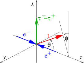
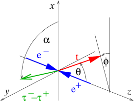
(a)(b)

Figure 1: Choice of the kinematics for the analysis of scalar particle (a) and unparticle interactions (b) with $\tan\alpha=-({\cal A}_{a}/{\cal A}_{b})\tan(d_{u}\pi)$, where ${\cal A}_{a,b}$ are given in Eq. (28).

4.2 CP violation and final state polarization

CP-odd contributions are also observed in the terms which depend on the final state top or antitop polarizations. These polarizations can be determined by analyzing the distributions of the final state charged leptons from the top (or antitop) decay. This method is viable in the top quark case because the top quark is so massive that it decays before it can hadronize, therefore avoiding masking nonperturbative effects. Of course, the observation of the CP violation through the measurement of the final state polarization means a loss of statistics. On the other hand, this shortage might be partly softened by the fact that most of the polarization depending terms are not proportional to the top mass and can be quite large as compared to terms independent of the top polarization.

If we divide the polarization vector $\vec{s}$ of the final top or antitop quark into a longitudinal and a transverse part,

$$\vec{s}=\vec{s}_{L}+\vec{s}_{T}=\frac{E}{Mp}h\vec{p}+\vec{\tau},$$ (31)

there is only a single term in both ${\cal B}_{a}$ and ${\cal B}_{b}$ that depends on $\vec{s}_{L}$. While $\vec{p}\cdot\vec{s}_{L}\vec{p}-p^{2}\vec{s}_{L}=0$, the factor

$$\vec{p}\cdot\vec{s}_{L}\vec{p}-E^{2}\vec{s}_{L}=-\frac{EMh}{p}\vec{p}$$ (32)

is proportional to the top mass. This factor is multiplied by the $\vec{\tau}_{+}$- and $\vec{\tau}_{-}$-dependent expressions (21) in the particle and both (21) and (22) in the unparticle case. Besides this, the terms containing these factors are $c_{P}$-dependent and therefore, as mentioned in point 5 of Sec. 3.1, have different signs if both the contributions from top and antitop polarization measurements are given by the top parameters ($\vec{p},\theta$). Due to this the CP-odd terms depend on $(\vec{\tau}_{-}+\vec{\tau}_{+})$ in the combinations $h\hat{k}\times(\vec{\tau}_{-}+\vec{\tau}_{+})\cdot\vec{p}$ for the particle case and in addition on $h(\vec{\tau}_{-}+\vec{\tau}_{+})\cdot\vec{p}$ for the unparticle case.

The terms depending on the transverse polarization of the final top (antitop) are not proportional to the top mass. One can divide these terms into $c_{S}$-dependent and $c_{P}$-dependent parts. In the $c_{S}$-dependent terms the CP-odd parts depend on the difference of the $\vec{\tau}_{-}$ and $\vec{\tau}_{+}$ vectors while in the $c_{P}$-dependent parts they depend on the sum of these vectors. However, the CP-odd parts in the corresponding terms of scalar particle and scalar unparticle contributions depend differently on these vectors. If the CP-odd part of some scalar particle contribution term contains the factor $\vec{\tau}_{-}-\vec{\tau}_{+}$ (or $\vec{\tau}_{-}+\vec{\tau}_{+}$), the corresponding term in unparticle case depends in addition on $\hat{k}\times(\vec{\tau}_{-}-\vec{\tau}_{+})$ (or $\hat{k}\times(\vec{\tau}_{-}+\vec{\tau}_{+})$) and vice versa. This circumstance might enable one, at least in principle, to separate CP-odd asymmetries in scalar particle and unparticle cases.

5 Final state polarizations

In this section we consider the actual polarizations of the final top or antitop quarks. The final quark polarizations provide additional tools for studying the mechanisms of the process and for separating the anomalous coupling contributions from the SM ones. It is well known that in the Born approximation the process $e^{+}e^{-}\to t\bar{t}$ with unpolarized or longitudinally polarized initial beams produces final quarks with polarization vector lying in the scattering plane [17]. When using TP beams the TP vectors $\vec{\tau}_{-}$ and $\vec{\tau}_{+}$ move the final top or antitop polarization vectors out of scattering plain. Therefore, in the approximation used the deviation of the final quark polarization vectors from the reaction plain is only due to the TP initial beams. SM contributes to TP-dependent terms only if both of the initial beams are transversely polarized. If only one of the initial beams is transversely polarized, such a deviation would indicate the presence of anomalous couplings.

5.1 Top polarization for the SM

Let us consider the final state polarization in more detail at the threshold of the process. At threshold the analytical expressions for the differential cross sections in Eqs. (13), (17) and (19) simplify considerably and the polarization properties of the quarks are displayed more clearly. We start our investigations from the SM sector considering the polarization properties of the top (antitop) quarks more generally. Since the TP-dependent terms vanish at the threshold, the main question will be how much one can tune the top (antitop) quark polarization by varying the LP parameters $h_{+}$ and $h_{-}$ of the initial beams. Indeed, the result for the polarization turns out to depend effectively on the parameter

$$\chi=\frac{h_{+}-h_{-}}{1-h_{+}h_{-}}.$$ (33)

At threshold the squared SM amplitude takes the form

$$|\mathcal{M}_{SM}|^{2}|_{\mathrm{thres}}=24M^{4}\left[A_{1}+A_{2}-2A_{4}\hat{k}\cdot\vec{\xi}\right],$$ (34)

where $\vec{\xi}$ is the top quark polarization vector and $K_{\gamma}$ and $K_{Z}$ have their threshold forms

$$K_{\gamma}=\frac{e^{2}}{6M^{2}},\qquad K_{Z}=-\frac{e^{2}}{\sin^{2}(2\theta_{W})(4M^{2}-M_{Z}^{2})}.$$ (35)

Using the method given in Ref. [11] one can find the magnitude and direction of the actual polarization vector of the top quark,

$$\vec{\xi}_{SM}=-\frac{B(\chi)\hat{k}}{A(\chi)},$$ (36)

where

$$A(\chi) = \frac{A_{1}+A_{2}}{2(1-h_{+}h_{-})}\ =\ a_{1}+a_{2}\chi,$$

$$B(\chi) = \frac{A_{4}}{1-h_{+}h_{-}}\ =\ a_{1}\chi+a_{2}$$ (37)

with

$$a_{1} = K_{\gamma}^{2}+K_{Z}^{2}c_{V}^{2}(g_{V}^{2}+g_{A}^{2})+2K_{\gamma}K_{Z}c_{V}g_{V},$$

$$a_{2} = 2K_{Z}c_{V}g_{A}(K_{\gamma}+K_{Z}c_{V}g_{V}).$$ (38)

In Fig. 2 the dependence of $A(\chi)$ and $B(\chi)$ on $\chi$ is given.

Figure 2: The dependence of $A(\chi)$ and $B(\chi)$ on $\chi$.

For the SM sector we use the values of the coupling constants and other parameters as given by the Particle Data Group [18], $g_{V}=-0.037$, $g_{A}=-0.5$, $c_{V}=0.191$, $c_{A}=0.5$, $g=e/\sin\theta_{W}$, $\sin^{2}\theta_{W}=0.2415$, $M_{t}=171.2\hbox{\rm\,GeV}$, and $M_{Z}=91.2\hbox{\rm\,GeV}$. We draw the attention to the fact that for $\chi_{0}=-0.408$ we obtain $B(\chi_{0})=0$. Therefore, at this value, $\chi=\chi_{0}$, the top polarization in the process appears only due to the anomalous coupling contributions. At the same time $A(\chi_{0})$ is smaller than at the point $\chi=0$ and as a consequence the top polarization from anomalous couplings is larger than in the case of unpolarized initial beams.

Fig. 3 shows how much the top polarization vector can be tuned by $\chi$ as compared to the case $\chi=0$, where the polarization is given by [19]

$$\vec{\xi}_{SM}|_{\chi=0}=-0.408\hat{k}.$$ (39)

Figure 3: The top polarization in SM at threshold as a function of $\chi$.

The fact that the magnitude of the top polarization vector at $\chi=0$ given in Eq. (39) is equal to the value of $\chi$ at which $\vec{\xi}_{SM}$ vanishes is not an occasional coincidence but a consequence of the special shape of the structure functions $A(\chi)$ and $B(\chi)$ in Eqs. (5.1). The polarization function $\xi_{SM}$ in Eq. (36) is of the same shape as the reciprocal function

$$\chi(\xi_{SM})=-\frac{a_{1}+a_{2}\xi_{SM}}{a_{1}\xi_{SM}+a_{2}}.$$ (40)

As a consequence, $\xi_{SM}(\chi=0)=\chi(\xi_{SM}=0)=-a_{1}/a_{2}=-0.408$.

5.2 Anomalous coupling corrections to the SM top polarization

The anomalous scalar particle coupling corrections to the SM contribution at threshold are given by

$${\cal B}_{a}|_{\mathrm{thres}} = \pm 48M^{4}c_{P}\vec{\xi}\Big{\{}(K_{\gamma}+K_{Z}c_{V}g_{V})[g_{S}\hat{k}\times(\vec{\tau}_{-}+\vec{\tau}_{+})-g_{P}(\vec{\tau}_{-}-\vec{\tau}_{+})]+$$ (41)

$$\qquad+K_{Z}c_{V}g_{A}[g_{S}\hat{k}\times(h_{+}\vec{\tau}_{-}-h_{-}\vec{\tau}_{+})-g_{P}(h_{+}\vec{\tau}_{-}+h_{-}\vec{\tau}_{+})]\Big{\}}.$$

For the anomalous scalar unparticle corrections one obtains in addition

$${\cal B}_{b}|_{\mathrm{thres}} = \pm 48M^{4}c_{P}\vec{\xi}\Big{\{}(K_{\gamma}+K_{Z}c_{V}g_{V})[g_{S}(h_{+}\vec{\tau}_{-}-h_{-}\vec{\tau}_{+})+g_{P}\hat{k}\times(h_{+}\vec{\tau}_{-}+h_{-}\vec{\tau}_{+})]+$$ (42)

$$\qquad+K_{Z}c_{V}g_{A}[g_{S}(\vec{\tau}_{-}+\vec{\tau}_{+})+g_{P}\hat{k}\times(\vec{\tau}_{-}-\vec{\tau}_{+})]\Big{\}}.$$

For $h_{-}=h_{+}=0$, the corresponding corrections to the top polarization vector are

$$\vec{\xi}_{p}=K_{p}\vec{\xi}_{a},\qquad\vec{\xi}_{u}=K_{u}(\cos(d_{u}\pi)\vec{\xi}_{a}+\sin(d_{u}\pi)\vec{\xi}_{b})$$ (43)

with

$$\vec{\xi}_{a} = \frac{{\cal A}_{a}c_{P}}{A(0)}[g_{S}\hat{k}\times(\vec{\tau}_{-}+\vec{\tau}_{+})-g_{P}(\vec{\tau}_{-}-\vec{\tau}_{+})],$$

$$\vec{\xi}_{b} = \frac{{\cal A}_{b}c_{P}}{A(0)}[g_{S}(\vec{\tau}_{-}+\vec{\tau}_{+})+g_{P}\hat{k}\times(\vec{\tau}_{-}-\vec{\tau}_{+})],$$ (44)

where ${\cal A}_{a,b}$ are defined in Eq. (28). In calculating values for the polarizations, we have to give values to the anomalous coupling constants $g_{S}$, $g_{P}$, $c_{S}$ and $c_{P}$. Scalar particle couplings arise in many extensions of the SM. However, up to now there exist no definite predictions about their values [3]. On the other hand, the unparticle phenomenology stands beyond the other SM extension models. Therefore, one has to make here quite voluntary presumptions that do not lay on definite theoretical grounds. Here we use the “SM-connected” setting $g_{S}=g_{V}$, $g_{P}=g_{A}$, $c_{S}=c_{V}$, $c_{P}=c_{A}$, and $g_{p}=g_{u}=g$.

The corrections to the top or antitop quark polarization due to anomalous couplings are transverse to the top (antitop) quark polarizations due to the SM which is antiparallel to the direction $\hat{k}$ of the initial beams. The angle between these two components is

$$\tan\varphi_{p,u}=\frac{|\vec{\xi}_{p,u}|}{|\vec{\xi}_{SM}|}.$$ (45)

Using $h_{\pm}=0$, $\tau_{+}=0$ and $\tau_{-}=0.8$ in order to eliminate the TP dependent SM terms also close to the exact threshold, the vector $\vec{\xi}_{u}$ is a vector in the plane spanned by $\vec{\tau}_{-}$ and $\hat{k}\times\vec{\tau}_{-}$ orthogonal to $\hat{k}$. However, a better reference frame to consider is the one spanned by the orthonormal basis

$$\hat{e}_{a}=\frac{g_{S}\hat{k}\times\vec{\tau}_{-}-g_{P}\vec{\tau}_{-}}{\sqrt{g_{S}^{2}+g_{P}^{2}}|\vec{\tau}_{-}|},\qquad\hat{e}_{b}=\frac{g_{S}\vec{\tau}_{-}+g_{P}\hat{k}\times\vec{\tau}_{-}}{\sqrt{g_{S}^{2}+g_{P}^{2}}|\vec{\tau}_{-}|}$$ (46)

The situation is illustrated in Fig. 4.

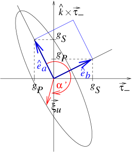
Figure 4: The vector $\vec{\xi}_{u}$ in the plane spanned by $\vec{\tau}_{-}$ and $\hat{k}\times\vec{\tau}_{-}$ for exemplary values for $c_{S}$ and $c_{P}$ and arbitrary scale for the coefficients, where $\tan\alpha^{\prime}=({\cal A}_{b}/{\cal A}_{a})\tan(d_{u}\pi)$.

For different values of $d_{u}$ the vector runs on a ellipse with half axis of length ${\cal A}_{a}\sqrt{g_{S}^{2}+g_{P}^{2}}|\vec{\tau}_{-}|$ along $\hat{e}_{a}$ and half axis of length ${\cal A}_{b}\sqrt{g_{S}^{2}+g_{P}^{2}}|\vec{\tau}_{-}|$ along $\hat{e}_{b}$. The angle in negative mathematical order with respect to $\hat{e}_{a}$ is given by $\alpha^{\prime}$, where $\tan\alpha^{\prime}=({\cal A}_{b}/{\cal A}_{a})\tan(d_{u}\pi)$. Together with the $d_{u}$-dependence given by $K_{u}$ in Eq. (45) we can calculate the dependence of the deviation angle $\varphi_{u}$ on $d_{u}$ in the region $1\leq d_{u}<2$ for different values of the scale $\Lambda_{u}$. The result is shown in Fig. 5.

Figure 5: Deviation angle $\varphi_{u}$ in dependence on $d_{u}$ for scales $\Lambda_{u}=2$, $3$, $5$, and $10\hbox{\rm\,TeV}$

Figure 6: Scale $\Lambda_{u}$ in dependence on the deviation angle $\varphi_{u}$ for unparticle dimensions $d_{u}=1.3$, $1.5$, $1.7$, and $1.9$

Figure 7: Scale $\Lambda_{p}$ in dependence on the deviation angle $\varphi_{p}$

The angle $\varphi_{u}$ turns out to be very sensitive to the dimension $d_{u}$, increasing rapidly if $d_{u}$ is going to $d_{u}=1$. The fine structure of the dependence close to $d_{u}=1.1$ is due to the elliptical dependence of the vector $\vec{\xi}_{u}$ on $d_{u}$, superposed by the increase of $K_{u}$ for $d_{u}\to 1$. Apparently, close to $d_{u}=1$ the value of the angle does no longer depend on the scale $\Lambda_{u}$ but takes a constant value because, using $\lim_{d_{u}\to 1}\sin(d_{u}\pi)\Gamma(1-d_{u})=-\pi$, $K_{d_{u}=1}$ is given by $K_{1}=-g_{u}^{2}/4k^{2}$. In Fig. 6 we show the dependence of the scale $\Lambda_{u}$ on the deviation angle $\varphi_{u}$ for the values $d_{u}=1.3$, $1.5$, $1.7$, and $1.9$. Again, the strong dependence on $d_{u}$ is obvious. Assuming that new physics is expected to appear at a scale of about $7\hbox{\rm\,TeV}$, the detection of effects for $d_{u}=1.7$ and $1.9$ requires a high angle resolution which may be not available for the near-future colliders. On the other hand, anomalous scalar particle coupling effects for the same assumed new-physics scale can be observed. This can be seen from Fig. 7 where the dependence of the scale $\Lambda_{p}$ on the deviation angle $\varphi_{p}$ is shown.

6 Conclusion

Our studies once more demonstrate the utility of using transversely polarized initial beams for searching new-physics indications. The additional directions provided by transverse polarization vectors can be successfully used for constructing new measurable quantities both in the presence of final top (antitop) polarization and its absence. In the previous case one loses statistics but gains other advantages in separating anomalous coupling signals from the SM contributions. The anomalous coupling contributions depend linearly on the transverse polarization vectors. This circumstance enables one to take only one of the initial beams to be transversely polarized. Such a choice eliminates the transverse polarization depending SM contributions. As an illustrative example we showed how to estimate the anomalous scalar particle and unparticle coupling manifestations through the measurement of the top quark polarization near the threshold of the process.

Acknowledgements

The work is supported by the Estonian target financed projects No. 0180013s07 and No. 0180056s09 and by the Estonian Science Foundation under grant No. 6216.

References

- [1] G.V. Dass and G.G. Ross, Phys. Lett. B57 (1975) 173; Nucl. Phys. B118 (1977) 284
- [2] K.i. Hikasa, Phys. Rev. D33 (1986) 3203
- [3] B. Ananthanarayan and S.D. Rindani, Phys. Rev. D70 (2004) 036005
-
[4]
H. Georgi,
Phys. Rev. Lett. 98 (2007) 221601;
Phys. Lett. B650 (2007) 275 - [5] H. Georgi and Y. Kats, “Unparticle self-interactions”, arXiv:0904.1962 [hep-ph]
- [6] H. Georgi and Y. Kats, Phys. Rev. Lett. 101 (2008) 131603
- [7] F. Sannino and R. Zwicky, Phys. Rev. D79 (2009) 015016
- [8] A. E. Nelson, M. Piai and C. Spitzer, Phys. Rev. D80 (2009) 095006
- [9] R. Zwicky, J. Phys. Conf. Ser. 110 (2008) 072050
- [10] K. Huitu and S.K. Rai, Phys. Rev. D77 (2008) 035015
- [11] I. Ots, H. Uibo, H. Liivat, R.K. Loide and R. Saar, Nucl. Phys. B588 (2000) 90
- [12] K. Cheung, W.Y. Keung and T.C. Yuan, Phys. Rev. D76 (2007) 055003
-
[13]
J.H. Christenson, J.W. Cronin, V.L. Fitch and R. Turlay,
Phys. Rev. Lett. 13 (1964) 138 - [14] H. Miyake et al. [Belle Collaboration], Phys. Lett. B618 (2005) 34
- [15] B. Aubert et al. [BaBar Collaboration], Phys. Rev. Lett. 95 (2005) 151804
- [16] A.E. Blinov and A.S. Rudenko, arXiv:0811.2380 [hep-ph]
-
[17]
M. Fischer, S. Groote, J.G. Körner, M.C. Mauser and B. Lampe,
Phys. Lett. B451 (1999) 406 - [18] C. Amsler et al. [Particle Data Group], Phys. Lett. B667 (2008) 1
- [19] R. Harlander, M. Jeżabek, J.H. Kühn and M. Peter, Z. Phys. C73 (1997) 477