The intermediate evolution phase in case of truncated selection.

Abstract

Using methods of statistical physics, we present rigorous theoretical calculations of Eigen’s quasispecies theory with the truncated fitness landscape which dramatically limits the available sequence space of a reproducing quasispecies. Depending on the mutation rates, we observe three phases, a selective one, an intermediate one with some residual order and a completely randomized phase. Our results are applicable for the general case of fitness landscape.

I Introduction

Developing realistic evolution models poses an important challenge for evolution research DBEH01 ; ei02 ). After the seminal work by Eigenei71 and successful experiments with the self-replication of macromoleculesMPS67 ; Bie87 , several theoretical studies attempted to explain this molecular evolution phenomenon [6-18]. Realistic fitness landscapes are not smooth, include neutral and lethal types, as observed in recent experimental studies with RNA virusesdo03 ; mo04 ; PGCM07 . In the most of evolution articles symmetric fitness landscapes are considered, where the fitness is a function of the Hamming distance from the wild (reference) sequence. While solving evolution models, the vast majority of results for the mean fitness have been derived using uncontrolled approximations even for the symmetric fitness landscapes, with too simplified sequence space wa93 and ignoring back mutationsei89 . A simplified geometry with only two (Hamming) classes for sequences with nonzero fitness was used in studies that investigate the role of lethal mutants in evolutionsu06 . Furthermore, in most evolution models the whole sequence space is assumed to be available for the evolving genome. However, the sequence space a limited population can use is severely restricted to a small part of the sequence space surrounded by an unsurmountable moat of lethal mutations. In this paper, we attempt to rigorously solve this case of a truncated fitness landscape for symmetric fitness landscape.

II The system

In Eigen’s theoryei71 ; ei89 , an information carrier reproduces with a certain rate $r_{i}$, producing offspring of the parental type with the probability $Q_{ii}$ and offspring of another (mutant) type $k$ with the probability $Q_{ki}$,

$$dx_{i}/dt=\{Q_{ii}r_{i}-\sum_{k}r_{k}x_{k}(t)\}x_{i}(t)+\sum_{k\neq i}Q_{ik}r_{k}x_{k}(t)$$ (1)

The whole sequence space contains $M=4^{L}$ different sequences, where $L$ is the genome length. The mean fitness of the system is $R=\sum_{k}r_{k}x_{k}(t)$ where $x_{i}$ are the relative frequencies of the different genotypes ($\sum_{k=0}^{4^{L}-1}x_{k}=1$). The master type $0$ has the maximal fitness $r_{0}$, and its copying fidelity is $Q\equiv Q_{00}=q^{L}$, where $q$ is the average incorporation fidelity and $L$ the chain length. It is convenient to work with the error rate $u\equiv L(1-q)$, leading to $Q=e^{-u}$. In this article we consider only the case $L\to\infty$, $u$ is finite. Eigen maps each genotype precisely into a node on the L-dimensional hypercube and has thus the correct connectivity for each type. The minimal number of steps leading from one position $i$ in sequence space to another one, $j$, is the Hamming distance $d_{ji}$.

In the evolution process the information content of the population can be maintained only when the selection force is higher than the dissipating one (mutation). Otherwise, above the error threshold, the information gets lost.

It has been shown that the system of nonlinear differential equations in Eq. 1 can be transformed to an infinite system of linear equations, connecting Eigen’s model with statistical mechanicsleut87 ; ta92 . For a single peak fitness landscape ($r_{0}=A$ and $r_{i\neq 0}=1$), the following condition for conserving the master sequence in the population holds ei71 ; ei89 :

$$AQ>1$$ (2)

where $AQ=1$ is the error threshold.

At the selective phase one has dr01

$$x_{0}=\frac{QA-1}{A-1}\sim 1,$$ (3)

and $x_{i}\sim 1/L^{d}$ for $d\ll L$, where $d$ is the Hamming distance from the wild sequence, see Eq. (21) in sh06 . We choose the sequences with $1\leq l\leq L$ from the corresponding $l$-th Hamming classes. A scaling by Eq.(3) exists also for the rugged (Random Energy Model like) fitness landscapes [11]. Scaling like the one in Eq. (3) has been applied in models of population genetics with few alleles. In realistic fitness landscapes, however, the wild type is present only in a few percents. Assuming neutrality, we can attain such scaling: a substantial fraction of one mutation neighbors of the wild sequence have the same high fitness. Neutrality increases the probability of such mutants and suppresses $x_{0}$ as low as

$$x_{0}\sim 1/\sqrt{L}.$$ (4)

This result could be derived easily using Eq. (6) in nc99 , for the case when there is a central neutral sequence and large fracture of neutral sequences among the neighbor sequences of the central sequence.

In non-selective phase one has

$$x_{0}\sim 1/M,$$ (5)

where $M$ is the total number of sequences, $M=4^{L}$.

The error threshold phenomenon closely resembles the ferromagnetic-paramagnetic phase transitionei89 , where the fitness of the system corresponds to the microscopic energy of the physics system, the mean fitness of the quasispecies to the free energy, and the mutation rate to temperature. To identify the different phases in statistical physics one uses the free energy and also the order parameters. A phase transition occurs when, during a change of temperature, the analytical expression of the free energy changes. Order parameter changes also: while magnetization is non-zero in the ferromagnetic phase, it is zero at high temperatures and in the absence of a magnetic field. A phase transition in evolution is identified by observing the mean fitness $R=\sum_{i}x_{i}r_{i}$ and choosing proper order parameters, for instance the degree of distribution around the master sequence, the surplus production, $s=\sum_{i}x_{i}(1-2d_{0i}/L)$, where $d_{0i}$ is the Hamming distance from wild type.

Instead of the 4-letter alphabet of genotypes, we consider only two symbols in a genome, the spins ”+” and ”–”, thus now $M=2^{L}$ [8]. Base substitutions correspond to sign changes of the spins. It is particulary easy to analyze landscapes where the fitness values are simple functions of the Hamming distance [8]. The N-dimensional sequence space is then transformed into a quasi-one-dimensional, linear chain of mutant classes $l$ where $p_{l}=N_{l}x_{l}$ comprises all types with the Hamming distance number $l$ from the master and the fitness value $J_{l}$. $N_{l}=\frac{L!}{l!(L-l)!}$ is the number of different genotypes in the class. The parameter $l$ can be identified as a phenotype parameter.

There is a principal difference between quasi-one dimensional model, derived rigorously from the initial sequence space with $2^{N}$ sequences and the one-dimensional one considered in [22] and other articles. In contrast to other one-dimensional models used earlier wa93 where each class contains only one type, in our case any class $l$ is composed of $N_{l}$ types and thus retains the connectivity; the Hamming distance between two sequences in the same class can take any value from $0$ to $2l$. Moreover, when evolution equations are formulated for class probabilities, the effective mutation rates to the lower class, $\sim(L-l)/L$, and to the higher class, $l/L$ are different and change with $l$ bw01 ,hi96 . In contrary, in the one-dimensional model of [22] these mutation rates are l-independent.

In our quasi-one dimensional model $J_{l}$ can be transformed into the $f(k)$ where $f(k)$ is an appropriate smooth function with the maximum at $k=1$, and $f(0)=1$. The ”magnetization” parameter $k$ is defined as $k\equiv(1-2l/L)$. A correct version of 1-dimensional evolution model has been suggested first in hi96 , the discrete time version of parallel model with a linear fitness.

Consider now the solution of the Eigen model with symmetric fitness landscape. The mean fitness $R$ for the fitness function $f$ has been derived as follows: sh06

$$R=\max\{f(k)Q^{(1-\sqrt{1-k^{2}})}\}|_{-1\leq k\leq 1}.$$ (6)

$s$ can be identified from the mean fitness expression using an equation

$$f(s)=R$$ (7)

as has been derived in bw01 for the parallel model. Thus in Eq.(6) the maximum is at some $k_{0}$, an order parameter of the system quantifying the bulk spin magnetization, while the surplus $s$ corresponds to the surface magnetization. Eq. (6) is an exact expression (at the infinite genome limit), while in other studies ei89 ; su06 back mutations have been ignored. As shown by Tarazonata92 , the Eigen model is not equivalent to the simple ferromagnetic system of spins in the lattice, but only to those spins interacting both inside the bulk of the lattice, and on the surface of the lattice. In this work, different phases will be characterized by $R$, the mean fitness, by $k_{0}$, the bulk magnetization, by $x_{0}$, the fraction of the wild type of the total population and by $s$, the surplus. When $k_{0}=0$, resulting in $s=0$, the population spreads statistically in sequence space, indicating a non-selective phase.

We gave the mean fitness and error threshold (when $s$ in Eq. (7) becomes 0) for the symmetric fitness landscape. The point is that this transition has also information theoretical meaning. Eigen actually found the error threshold from information theoretical consideration of his model. Eigen’s idea (information theoretical content of a model) resembles the investigation of information theoretical (optimal coding) aspects of disordered systems, developed in statistical physics two decades laterso89 ; sa92 . In the Random Energy Model of spin glass de81 the phase transition point was derived using the information theory analogy so89 ; sa92 , and was found to yield results corresponding to those derived by Eigen. The deep information theoretical meaning of error threshold transition in evolution models (equivalent to Shannon inequality for optimal coding) is a solid argument that transition like the one by Eq. (2) exists for any (irregular, with lethal or neutral mutants) fitness landscapes.

III Wagner & Krall theorem.

Wagner & Krall wa93 considered a population composed of the master and an infinite linear chain of mutants, where each type mutates only to its next neighbor and the fitness $r_{i}$ decreases monotonically. When there is no low bound of the fitness, an absence of the error threshold transition was derived. Indeed, when in Eq. 6 $f(0)=0$, there is no error threshold transition. But in more general symmetric fitness landscapes with a finite $f(0)$, this ceases to be valid. The proof is as follows: the maximum of types are located at the Hamming distance class $L/2$ or, equivalently, at $k=0$. Consider the logarithm of the right hand side in Eq. 6, and expand near $k=0$:

$$(1-\sqrt{1-k^{2}})\ln Q+\ln f(k)\approx-u\frac{k^{2}}{2}+\ln(f(0))+ck^{\epsilon}$$ (8)

where $c$ and $\epsilon$ are parameters describing the function $f(k)$, and $\ln f(k)-\ln f(0)\sim ck^{\epsilon}$ at $k\to 0$. When the fitness decreases slowly and so $\epsilon<2$, Eq. 8 has a maximum at $k>0$, fulfilling the condition for selection. When $\epsilon\geq 2$, it can be demonstrated that there is a maximum at $k=0$ for a sufficiently low reproduction fidelity $Q$, therefore a sharp error threshold transition results. In the too simplistic model of Wagner & Krall, the right hand side of Eq. 8 lacks the quadratic term, resulting in a monotonic function of $k$ and the absence of phase transition. In the Eigen model the quadratic term holds, breaking the monotonic character of $R$ in Eq. 8 and invoking the error threshold.

IV Truncated single peak fitness landscape.

Let us consider a symmetric fitness landscape, where there is non-zero fitness only to some Hamming distance from the reference sequence. Here we define the truncated landscape as a single-peak one where all sequences beyond the Hamming distance $d\equiv L(1-K)/2$ are lethal:

$$r_{l}=1\quad 1\leq l\leq d,\qquad r_{l}=0\quad l>d$$ (9)

Now we have

$$M=\frac{L!}{d!(L-d)!}$$ (10)

non-lethal sequences.

To define the mean fitness, we compare the expression of Eq. (6) inside the region $K<k<1$ and at the border.

The investigation of this model is instructive, see Figs. 1-4.
When $QA>1$ the phase is selective (phase I), $x_{0}$ is given by Eq.(3), $k_{0}=1$, $R=QA$, see ki66 .
When

$$1>QA>Q^{1-\sqrt{1-K^{2}}},$$ (11)

a new phase II prevails with

$$k_{0}=1,R=QA$$ (12)

In the II phase $x_{0}$ is decreasing exponentially with L. The expression of $x_{0}$ is calculated in the appendix,

$$x_{0}=\exp[\int_{K}^{1}dm\frac{1}{2}\ln\frac{\frac{\ln A}{u}+\sqrt{\frac{(\ln A}{u})^{2}-1+m^{2}}}{1+m}]$$ (13)

At the the transition point (to the II phase) the expression in the exponent is becoming zero, therefore the transition is continuous. When

$$QA<Q^{1-\sqrt{1-K^{2}}},$$ (14)

the maximum is at the border and we have the non-selective phase III,

$$k_{0}=K,R=Q^{1-\sqrt{1-K^{2}}}$$ (15)

The expression for $x_{0}$ is defined in the appendix, Eq.(A14). There is some focusing around reference sequence, and $x_{0}$ is higher than $1/M$. For $K=0.9$ we obtained $x_{0}\approx 1/M^{2/3}$.
The transition between II and III phases is a discontinuous one, $x_{0}$ decreases $M_{1}$ times, see Eq. (A21)

$$M_{1}\sim\exp[L\int_{K}^{1}dm\frac{1}{2}\ln\frac{\sqrt{1-K^{2}}+\sqrt{m^{2}-K^{2}}}{\sqrt{1-K^{2}}-\sqrt{m^{2}-K^{2}}}]$$ (16)

Fig.4 illustrates different behavior of $x_{0}$ in three phases.

While in the ordinary Eigen model (without truncation of fitness) there is a sharp phase transition with the jump of the $x_{0}$ behavior from the Eq.(3) to the $1/M$, in truncated case these sharp transition is moved to the transition point between II and III phases. Now $x_{0}$ is continuous at transition point between I and II phases. For the Summers-Litwin case with $K=1$ we have $M_{1}\to 1$, therefore the transition disappears as has been obtained in su06 , and for the $K=0$ case we get the result of Eigen model $M_{1}=1/2^{N}$. Our formulas are derived for the case $K\geq 0$.

Is phase II a selective one in the ordinary meaning? Clearly, its mean fitness is higher than in a typical non-selective phase like phase III. This point was clarified by calculating the surplus, replacing the step-like fitness function near the borderline ($k=K$) with a smooth function $f(k)$ which changes its value from 1 to 0 near $K$. In both phases, II and III, with $QA>Q^{1-\sqrt{1-K^{2}}}$, the majority of the population is near the borderline, both on the viable and the lethal side. Therefore, while there is a kind of phase transition with some population rearrangement, phase II is identified as an intermediate one, with $x_{0}\ll 1$, as in the non-selective phase. Summers and Litwin su06 first realized that $k_{0}\to 1$ in a truncated fitness landscape and tried to analyze the phenomenon. Unfortunately, they used too simplistic a model where all mutants except the nearest neighbors of the master type were lethal. Fig. 2 compares the relative concentration of the master at various superiorities in the single-peak fitness landscape described in ei71 ; ei89 , with the truncated fitness landscape with $d=8$, and the case considered by Summers and Litwin. Note the strong dependence of the master concentration on the master superiority in the more realistic landscape, leading to an error threshold, in contrast to the case in su06 . The population profiles of the truncated fitness landscape at different mutation rates are shown in Fig. 3, showing the transition from a master-dominated population via a wide-spread mutant distribution to a non-selective case.

In the Table1 we give the results of numeric for different phases. Mean fitness is well confirmed numerically, while the accuracy of numerics is poor to get correct values of $x_{0}$ in the second phase, $2.37<A<2.77$.

Figure 1: Phase structure for the model with the overlap parameter for truncation point $K=0.9$, and mutation rate $u=1$. I: selective phase with $QA>1$, $A$ is the fitness at the peak, $Q=e^{-u}$ is the errorless copying probability of the genome. II: Intermediate phase with $QA<1$ and $QA>Q^{1-\sqrt{1-K^{2}}}$. III: non-selective phase with $QA<Q^{1-\sqrt{1-K^{2}}}$.

Figure 2: Semilogarithmic plot of $x_{0}$ versus $A$ for a single peak fitness landscape truncated at $d>8$ with $u=1,L=3000$. The upper curve corresponds to the Summers-Litwin model, the middle curve to the truncated fitness landscape as in Fig. 3. The square boxes correspond to a single peak fitness model. For $\ln(A)<1$ Eigen model with single peak fitness has $x_{0}=0$.

Figure 3: Truncated Eigen model with $d=8$, $A=3,u=1,L=3000$. The distribution of probabilities of Hamming classes $p_{l}$ at different mutation rates ($u$ values). At high accuracy (circles) the population groups around the master type, at intermediate accuracy the population peaks at the truncation border, at low accuracy the master type has practically disappeared and the majority of the progeny is lethal.

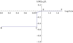
Figure 4: The graphics of $\ln x_{0}/L$ for the truncated Eigen model at infinite $L$ with $K=1/2,u=1$. The I phase (curve BC) is at $1<\ln A/u$, the second (curve DE) at $1<0.88<\ln A/u<1$ and the third (curve EF)at $0<\ln A/u<0.88$. The curve CD corresponds to the jump at the border between II and III phases. In the first phase $\ln x_{0}/L\sim O(1/L)$.

Phase	III	III	II	II	II	II	I
A	2.2	2.3	2.4	2.5	2.6	2.7	2.8
R	0.859	0.859	0.883	0.919	0.957	0.993	1.030
R th.	0.875	0.875	0.882	0.919	0.956	0.992	1.029
$x_{0}$	$4*10^{-117}$	$7*10^{-54}$	$2*10^{-24}$	$4.7*10^{-16}$	$10^{-9}$	$4.4*10^{-4}$	0.0167
$x_{0}$ th.							0.0164

Table 1: Eigen model with truncated single peak fitness landscape for $L=1000,u=1,K=1/2$. The transition between I and second phases is at $A\approx 2.778$, between II and III phases at $A\approx 2.377$.

How the phases can be identified? The fact is that the parameters $k_{0}$ and $s$ have different meanings in a statistical physics approach. This subject has been well analyzed in a series of articles by E. Baake and her co-authors. $s$ and $k_{0}$ have been identified with the transverse and longitudinal magnetizations of spins in the corresponding quantum model. We just link $s$ with the mean characteristic of the phenotype, and $k_{0}$- with the repertoire of genotypes. The consensus sequence should be determined experimentally not only via distribution $x_{i}$, but also via distribution $(x_{i})^{2}/\sum_{j=0}^{M}(x_{j})^{2}$. Consider

$$\hat{k}_{l}=\frac{N_{l}(x_{i})^{2}}{\sum_{j}(x_{j})^{2}},$$ (17)

where $x_{i}$ belongs to the phenotype class $l$ with $N_{l}$ different genotypes. Having such data, one can simply identify the phase structure.

In the appendix we solve the truncated fitness models for the general monotonic smooth function $f(x)$. The numerics confirms well our analytical results for the new phase.

V Discussion

We rigorously solved (at the infinite genome length limit) Eigen’s model for the truncated selection using the method of sh06 as well as methods of statistical mechanics, including the analogy of the error threshold to the ferromagnetic-para -magnetic transition. This analogy is a complicated critical phenomenon, presented by Leuthäusser and Tarazona leut87 ; ta92 and well analyzed by E. Baake and co-authors ba97 ; bw01 . Instead of using only one order parameter to identify the phase of the model, magnetization, it is necessary to take into account several order parameters describing the order of spins in the bulk lattice and at the surface. Recently the existence of an error threshold has been questioned su06 in the case of truncated selection. In this model the available sequence space has been shrunk to an extremely small size. Fig. 2 illustrates that the unrealistic assumption in su06 changed the relative concentration of the master type by more than 3 orders of magnitude. Nevertheless, this work was certainly useful for clarifying the concept of quasispecies: the authors first realized the intriguing features of a truncated selection landscape. We found a new evolution (intermediate) phase, when there is no successful selection via phenotype trait (the majority does not share the trait), while there is some grouping of population at genotype level. The intermediate evolution phase differs from the non-selective phase, the frequency of wild type being $\frac{1}{\sqrt{M}}$ or higher in the intermediate phase compared with $\sim\frac{1}{M}$ in the non-selective phase of Eigen model. We proposed a parameter to measure the hidden grouping of population in a genotype level, Eq. (17). Such hidden ordering could be important in case of changing environment: it is possible to force the whole population to extinction changing the fitness of a small fraction (much smaller than $1/L$, but much higher than $1/M$, M is the number of different genotypes) of viruses in the population. We recommend virologists to measure the consensus sequence not only using the the probabilities $x_{i}$, but also $x_{i}^{2}$. The evolution picture of the virus population is robust when two versions of consensus sequence are close to each other. In experiments do03 has been observed an evolution picture, qualitatively similar to the intermediate evolution phase.

How the error threshold transition is connected to the virus extinction in virus experiments, is another story. Several mechanisms are possible: an error catastrophe, as well as a critical mean fitness in order to maintain viral growth wi07 . In this work, we observed the new phase with single peak and symmetric landscapes, but this phase exists probably for any (including irregular) fitness landscape with a lethal wall in sequence space.

VI Acknowledgments

D.B. Saakian thanks the Volkswagenstiftung grant ”Quantum Thermodynamics” and the National Center for Theoretical Sciences in Taiwan and Academia Sinica (Taiwan) under Grant No. AS-95-TP-A07 for the financial support. We thank E. Domingo and M.W. Deem discussions.

Appendix A. Application of HJE for truncated symmetric landscape.

Let us apply the Hamilton-Jacobi equation (HJE) method sa07 ; sa08 to Eigen model with truncated symmetric fitness landscape. Consider a piecewise smooth, monotonic fitness function $f(m)$,

$$f(m)=f_{0}(m),m>K,$$

$$f(m)=0,m<K$$ (A.1)

Phase	III	III	II	II	II	I	I	I
c	0.5	1	1.2	1.3	1.5	1.9	2.1	3
ln(R)	-0.090	-0.016	0.0163	0.035	0.084	0.212	0.287	0.665
ln(R) th	-0.071	-0.009	0.0160	0.034	0.083	0.213	0.288	0.666
s	0.507	0.507	0.507	0.508	0.510	0.525	0.541	0.663
s th.	0.5	0.5	0.5	0.5	0.500	0.5	0.523	0.666
$-\ln(x_{0})$	223	199	185	177	160	131	120	84

Table 2: Eigen model with truncated fitness, $K=1/2,L=500,u=1,f(x)=\exp(cm^{2}/2)$. The transition between I and second phases is at $c=2$, between II and III phases at $c=1/\sqrt{1-K^{2}}\approx 1.1547$. In the I phase we have: $s=1/c,\ln(R)/u=c(1-1/c)^{2}/2$. In the II phase: $s=K,\ln(R)/u=c(1-1/c)^{2}/2$. In the III phase: $s=K,\ln(R)/u=cK^{2}/2+\sqrt{1-K^{2}}-1$.

Phase	III	III	III	II	II	II	I	I
c	0.5	1	2.2	2.4	2.5	2.6	3	4
ln(R)	-0.135	-0.016	-0.022	0.0202	0.0433	0.0676	0.172	0.459
ln(R) th	-0.11	-0.092	-0.042	0.0201	0.0435	0.0678	0.171	0.460
s	0.507	0.507	0.510	0.514	0.518	0.523	0.563	0.698
s th.	0.5	0.5	0.5	0.5	0.5	0.5	0.556	0.701
$x_{0}$	230	216	142	128	122	117	98	70

Table 3: Eigen model with truncated fitness, $K=1/2,L=500,u=1,f(x)=\exp(cm^{3})$. The transition point is at $c\approx 2.31,m_{0}=0.866$ in the model without truncation. The transition point between II,III is at $c\approx 2.79$.

Here $f_{0}(m)$ is a monotonic analytical function.

We denote by $k_{0}$ the maximum point in Eq.(6). As $s$ is defined by Eq. (7), for the monotonic fitness function we obtain

$$s\leq k_{0},$$ (A.2)

and there is only one solution of Eq. (7).

Using an ansatz

$$p_{l}=\exp[LU_{0}(m,t)],$$ (A.3)

$m=1-2l/L$, in sa07 has been derived the following equation

$$L\frac{\partial U_{0}(m,t)}{\partial t}=f_{0}(m)e^{-u}\times$$

$$\exp\{u[\cosh(2\frac{\partial U_{0}(m,t)}{\partial m})+m\sinh(2\frac{\partial U_{0}(m,t)}{\partial m})]\}$$ (A.4)

The HJE approach works for any piecewise smooth fitness functions. Eq. (A1) is such a case. To solve our truncated case we should just use different analytical solutions for the regions $-1<m<K$ and $K<m<1$.

Assuming an asymptotic $U_{0}(m,t)=\frac{R}{L}t+U(m)$, we derived sa07

$$R=f_{0}(m)e^{-u}\times$$

$$\exp\{u[\cosh(2\frac{dU(m)}{dk})+m\sinh(2\frac{dU(m)}{dm})]\},$$ (A.5)

where $R$ is derived by Eq.(6). The surplus $s$ is defined as the value of $m$ where $U(m)$ has a maximum. When $s$ is inside the region $[K,1]$, $U^{\prime}(s)=0$. At extremum points with $U^{\prime}(m)=0$ Eq.(A5) gives $f(s)=R$. As for a monotonic fitness function there is a single solution for Eq. (6), $U(x)$ has a single maximum point in this case, therefore it is a concave function and we take $U(s)=0$.

We use Eq.(A5) to define $p_{l}$ with an accuracy $O(1)$ for $\ln p_{l}$, calculating $U(m)=U(s)+\int_{s}^{m}U^{\prime}(m)dm$ for the corresponding $m=1-2l/L$. Moreover, it is possible to calculate $\ln p_{l}$ with a higher accuracy $O(1/L)$. In [18] we gave explicit formulas for the case of parallel model. It is possible to construct similar results for the Eigen model as well.

We have two branches of solutions for Eq. (A5):

$$U^{\prime}(m)=\frac{1}{2}\ln\frac{q\pm\sqrt{q^{2}-1+m^{2}}}{1+m},$$

$$q=\frac{1}{u}\ln\frac{R}{f(m)}+1$$ (A.6)

It is a principal point the choice of different solutions. We choose the proper branch assuming:

• U(m) is continuous function,

• U’(m) is continuous function,

• U(m) is a concave function for the monotonic fitness function $f(m)$.

The transition between two branches ($\pm$ solutions in Eq.(A5)) is only at the point where $q^{2}-1+m^{2}=0$ or

$$R=f(m)e^{-u+u\sqrt{1-m^{2}}}$$ (A.7)

According to Eq.(6), $R$ is the maximum of the right hand side. Thus we should choose only the branch with $"-"$ sign when $k_{0}$ is at the border, $k_{0}=K$. When k is inside the interval $[K,1]$, then we choose the $"-"$solution for the interval $[k_{0},1]$ and $"+"$ solution in the interval $[K,k_{0}]$.

For the $V(m)=\ln(\sqrt{N_{l}p_{l}})/L$ we have another equation [18],

$$R=f_{0}(m)e^{-u}\exp\{u[\cosh(2\frac{dV(m)}{dm})\sqrt{1-m^{2}}]\}$$ (A.8)

The minimum of the right hand side via $V^{\prime}$ just gives the $f(m)e^{-u+u\sqrt{1-m^{2}}}$. Thus at the maximum point $m=k_{0}$ of function $V(m)$ we have $V^{\prime}(k_{0})=0$. In this article we consider the case when Eq.(6) has a single solution $k=k_{0}$. Then $V(m)$ is a concave function.

Solution of equations (A5),(A7) are simply related,[18],

$$V(m)=U(m)+\frac{(1+m)\ln\frac{1+m}{2}}{4}+\frac{(1-m)\ln\frac{1-m}{2}}{4}$$ (A.9)

Consider now different phases of our model. The selective one with $K<k_{0}<1,K<s<1$; the non-selective one with $k_{0}=K,s=K$, and intermediate one with $K<k_{0}<1,s=K$.

Selective phase.

Now $R$ is given by Eq. (6) with a $K<k_{0}<1$. We used $"-"$ solution of Eq.(A6) for $k_{0}<m<1$ and the $"+"$ solution for $K<m<k_{0}$. The maximum points of both functions $U(m)$ and $V(m)$ are inside the interval $[K,1]$. We have $U^{\prime}(s)=0$ and $V^{\prime}(k_{0})=0$. The formulas for the steady state distributions are the same as in sa07 . We have a mean fitness

$$R=f(k_{0})e^{-u+u\sqrt{1-k_{0}^{2}}}$$ (A.10)

For the $p_{l},m=L(1-2l/L),k_{0}<m\leq 1$ we have an expression

$$p_{l}=\exp[L\int_{k_{0}}^{m}dm\frac{1}{2}\ln\frac{q-\sqrt{q^{2}-1+m^{2}}}{1+m}]$$

$$+L\int_{s}^{k_{0}}dm\frac{1}{2}\ln\frac{q+\sqrt{q^{2}-1+m^{2}}}{1+m}],$$

$$q=\frac{1}{u}\ln\frac{R}{f(m)}+1$$ (A.11)

For $m<k_{0}$ we have

$$p_{l}=\exp[L\int_{s}^{m}dm\frac{1}{2}\ln\frac{q+\sqrt{q^{2}-1+m^{2}}}{1+m}],$$

$$q=\frac{1}{u}\ln\frac{R}{f(m)}+1$$ (A.12)

Nonselective phase.

Now the maximum of Eq.(6) is at the border $k_{0}=K$, and we have

$$R=f(K)e^{-u+u\sqrt{1-K^{2}}}$$ (A.13)

We use $"-"$ solution of Eq.(A6) for the whole interval $K<m<1$. For the $p_{l},m=L(1-2l/L)$ we have an expression

$$p_{l}=\exp[L\int_{K}^{m}dm\frac{1}{2}\ln\frac{q-\sqrt{q^{2}-1+m^{2}}}{1+m}],$$

$$q=\frac{1}{u}\ln\frac{R}{f(m)}+1$$ (A.14)

and the maximum is for $p_{d}$ with $m\equiv\frac{1-2d}{L}=K$.

For the single peak fitness case ($f(1)=A$ and $f(m)=1$ for $m<1$), we have $q=\sqrt{1-K^{2}}$ and

$$x_{0}\equiv p_{0}\sim\exp[\frac{L}{2}\int_{K}^{1}dm\ln\frac{\sqrt{1-K^{2}}-\sqrt{m^{2}-K^{2}}}{1+m}]$$ (A.15)

For the $1/M$ we have an expression

$$\frac{1}{M}\sim\exp[\frac{L}{2}\int_{K}^{1}dm\ln\frac{1-m}{1+m}]$$ (A.16)

Intermediate phase. Now mean fitness is given by Eq.(6) with some $K<k_{0}<1$ and $s=K$. We used $"-"$ solution of Eq.(A6) for $k_{0}<m<1$ and $"+"$ solution for $K<m<k_{0}$. When $m>k_{0}$, we have

$$p_{l}=\exp[L\int_{K}^{k_{0}}dm\frac{1}{2}\ln\frac{q+\sqrt{q^{2}-1+m^{2}}}{1+m}+$$

$$L\int_{k_{0}}^{m}dm\frac{1}{2}\ln\frac{q-\sqrt{q^{2}-1+m^{2}}}{1+m}]$$ (A.17)

In case of $K<m<k_{0}$ we have

$$p_{l}=\exp[L\int_{K}^{m}dm\frac{1}{2}\ln\frac{q+\sqrt{q^{2}-1+m^{2}}}{1+m}]$$ (A.18)

We took $U(K)=0$, as the maximum of population is at the border with $m=K$.

For the SP case we have $q=\frac{\ln A}{u}$, and

$$x_{0}=\exp[L\int_{K}^{1}dm\frac{1}{2}\ln\frac{\frac{\ln A}{u}+\sqrt{\frac{(\ln A}{u})^{2}-1+m^{2}}}{1+m}]$$ (A.19)

Above the transition point $\ln A=\sqrt{1-K^{2}}$ Eq.(19) gives

$$x_{0}=\exp[L\int_{K}^{1}dm\frac{1}{2}\ln\frac{\sqrt{1-K^{2}}+\sqrt{m^{2}-K^{2}}}{1+m}]$$ (A.20)

We see that at the transition point there is a jump, $x_{0}$ decreases $M_{1}$ times,

$$M_{1}\sim\exp[L\int_{K}^{1}dm\frac{1}{2}\ln\frac{\sqrt{1-K^{2}}+\sqrt{m^{2}-K^{2}}}{\sqrt{1-K^{2}}-\sqrt{m^{2}-K^{2}}}]$$ (A.21)

For $K=0.5$ Eq.(A20) gives $\ln(x_{0})/L\approx-0.057$, while $\ln(M)/L\approx-0.56$. Thus above the transition point to the third phase

$$Log(x_{0})\sim\frac{1}{M^{0.1}}$$ (A.22)

Consider the case $K=0.99$. Now we have $\ln(x_{0})/L\approx-0.01$ and $\ln(M)/L\approx-0.031$. Thus

$$\ln(x_{0})\sim\frac{1}{M^{0.32}}$$ (A.23)

Consider evolution model with general fitness function $f(x)$. Assume that without truncation the error threshold transition is a discontinuous one, and there is a jump from non-zero $k_{0}>$ in selective phase to $k=0$ solution in Eq.(6) for non-selective phase. Let us introduce the truncation. Choosing $K<k_{0}$, we have three phases, see Table 3, and $x_{0}$ decreases $M_{2}$ times at the transition point between II and III phases,

$$M_{2}\sim\exp[L\int_{k_{0}}^{1}dm\frac{1}{2}\ln\frac{\sqrt{1-K^{2}}+\sqrt{m^{2}-K^{2}}}{\sqrt{1-K^{2}}-\sqrt{m^{2}-K^{2}}}]$$ (A.24)

If in the original (without truncation) model the error threshold transition is a continuous one with $k_{0}=0$, after truncation we have different expressions for $x_{0}$ in the II ($k_{0}>K,s=K$) and III ($k_{0}=K,s=K$) phases while continuous transitions $I\to II$ and $II\to III$, see Table 2. We have a similar behavior for the phase transitions in case of originally (without truncation) discontinuous error threshold transition, if the truncation parameter $K$ is chosen too large,$K>k_{0}$.

Let us derive an important constraint for the population of the class at the Hamming distance $n=L(1-k_{0})/2$. For the corresponding $V$ we have

$$V(k_{0})\equiv\frac{1}{L}\ln\frac{p_{n}}{\sqrt{N_{n}}}$$ (A.25)

As $p_{d}=1$ (the majority of population is at the border with the overlap parameter $K=(1-2d)/L$), we have

$$V(K)\equiv\frac{1}{L}\ln\frac{1}{\sqrt{M}},$$ (A.26)

as $M=N_{K}$. We proved before that $V(m)$ has a single maximum (in our case with a single solution for the maximum point $k$ in Eq. (6)). Thus

$$V(K)>V(k_{0})$$ (A.27)

which gives

$$p_{n}>\frac{\sqrt{N_{n}}}{\sqrt{M}}$$ (A.28)

The last inequality supports the choice of order parameter in Eq. (17).

For the single peak case $n=0$, and we get from Eq.(A28)

$$x_{0}>\frac{1}{\sqrt{M}}$$ (A.29)

Eqs.(A22,A23) give even higher values for $x_{0}$.

References

- (1) E. Domingo, C. K. Biebricher, M. Eigen, and J.J. Holland, Quasispecies and RNA Virus evolution: Principles and Consequences. (Landes Bioscience, Austin, TX, 2001).
- (2) M. Eigen, Proc. Natl. Acad. Sci. USA 99, 13374 (2002).
- (3) M. Eigen, Naturwissenschaften 58, 465 (1971).
- (4) C. K. Biebricher, Cold Spring Harbor Symp. Quant. Biol. 52, 299 (1987)
- (5) D.R. Mills, R. L. Peterson, and S. Spiegelman, Proc. Natl. Acad. Sci. USA 58, 217 (1967).
- (6) J. Swetina, and P. Schuster, Biophys. Chem. 16, 329 (1982).
- (7) I. Leuthäusser, J. Stat. Phys. 48, 343 (1987)
- (8) P. Schuster, and J. Swetina, Bull. Math. Biol. 50, 635 (1988).
- (9) P. Tarazona, Phys. Rev. A 45, 6038 (1992).
- (10) M. Eigen, J. S. McCaskill, and P. Schuster, Adv. Chem. Phys. 75, 149 (1989).
- (11) S. Franz, and L. Peliti, J. Phys. A 30, 4481 (1997).
- (12) E. Baake, M. Baake, and H. Wagner, Phys. Rev. Lett. 78, 559 (1997).
- (13) E. Baake, and H. Wagner, Genet. Res. 78, 93 (2001)
- (14) J. Hermisson, O. Redner, H. Wagner, and E. Baake, Theor. Pop. Biol. 62, 9 (2002)
- (15) D. B. Saakian, and C.-K. Hu, Proc. Natl. Acad. Sci. USA 103, 4935 (2006).
- (16) D. B. Saakian, E. Munoz, C.-K. Hu, and M. W. Deem, Phys. Rev. E 73, 041913 (2006).
- (17) J.-M. Park and M. W. Deem, PRL, 98, 058101(2007).
- (18) D.B. Saakian, Journal of statistical physics, 128,781(2007).
- (19) D. B. Saakian, O. Rozanova, and Andrei Akmetzhanov, Phys.Rev. E 78, 041908 (2008).
- (20) R. Sanjuan, A. Moya, and S. F. Elena, Proc. Natl. Acad. Sci. USA 101, 8396 (2004).
- (21) E. Lázaro, C. Escarmis, J. Perez-Mercader, S. C. Manrubia, and E. Domingo, Proc. Natl. Acad. Sci. USA 100, 10830 (2003).
- (22) M. Pariera, M., G. Fernandez, B. Clotet, and M. A. Martinez, Mol. Biol. Evol. 24, 382 (2007).
- (23) G. P. Wagner, and P. Krall, J. Math. Biol.32, 33 (1993).
- (24) J. Summers, and M. Litwin, J. Virol. 80, 20 (2006).
- (25) B. Drossel, Biological evolution and statistical physics Advances in Physics 50, 209 (2001).
- (26) E.V. Nimwegen, J.P.Crutchfield, and M. Huynen Proc. Natl. Acad. Sci. USA 96, 9716 (1999).
- (27) H. Woodcock and P.G. Higgs, J. Theor. Biol. 179:61-73, (1996).
- (28) N. Sourlas, Nature 339, 693 (1989).
- (29) D. B. Saakian, JETP Lett.55,2(1992).
- (30) B. Derrida, Phys. Rev. B 24, 2613 (1981).
- (31) Kimura and Maruyama. Genetics 54,1303(1966)
- (32) J. J. Bull, R. Sanjuan, and C. O. Wilke, J. Virol. 81, 2930 (2007).