Theory for wavelength-resolved photon emission statistics in single-molecule spectroscopy

Abstract

We derive the moment generating function for photon emissions from a single molecule driven by laser excitation. The frequencies of the fluoresced photons are explicitly considered. Calculations are performed for the case of a two level dye molecule, showing that measured photon statistics will display a strong and non-intuitive dependence on detector bandwidth. Moreover, it is demonstrated that the anti-bunching phenomenon, associated with negative values of Mandel’s Q-parameter, results from correlations between photons with well separated frequencies.

Single-molecule spectroscopy (SMS) Moerner and Orrit (1999) provides a detailed glimpse into our natural world. Typically, SMS experiments rely upon broadband detection of fluoresced photons to monitor molecular dynamics, however in studies of resonance energy transfer (RET) Ha et al. (1996) and semiconductor quantum dots Moreau et al. (2001) considerably more information can be obtained by resolving photon emission into two color channels. Recently Luong et al. (2005), multi-channel detection schemes have been introduced to extend the capabilities of SMS still further.

The information obtained by SMS is useful only if it can be readily interpreted. SMS has received considerable theoretical attention (see reviews Jung et al. (2002) and references within), but most of this work ignores any consideration of photon color. A notable exception is the treatment of RET, which has been considered in detail Gopich and Szabo (2005). A related treatment of “frequency resolved” photon counting, including quantum evolution of the molecule, has also been proposed by us Bel et al. (2006). However, these studies rely upon a direct correspondence between individual spectral transitions and experimental detection channels. This picture may be adequate for well resolved transitions and certain experimental conditions, but falls short of providing a complete theoretical description of emission spectroscopy at the single-molecule level.

Within the field of quantum optics, time correlations between spectrally resolved photons have been studied both experimentally Aspect et al. (1980) and theoretically Nienhuis (1993) for the case of resonance fluorescence from 2-level atoms. These studies also rely upon a direct correspondence between individual spectral transitions (in the dressed-atom picture Cohen-Tannoudji et al. (1992)) and the frequency of the emitted photons to enable elementary interpretation of experiment and simplified theoretical analysis. This letter introduces a general formalism to describe single molecule photon emission that does not presume simplifying characteristics of the molecular system or detection apparatus. Our results may be directly applied to model systems and lay the groundwork for development of controlled approximation schemes in the study of more complex condensed-phase systems.

In previous work, we Zheng and Brown (2003a) and others Cook (1981); Gopich and Szabo (2005) have introduced the generating function formalism for calculation of single-molecule photon counting statistics without spectral resolution. Such broadband photon statistics may be calculated by monitoring the number of times that spontaneous emission occurs as the molecule evolves. Within the Markovian limit for molecular dynamics, spontaneous emission is a simple rate process and these emission events may be treated purely classically, even though the underlying dynamics may involve facets of quantum evolution. Calculation of photon counting moments proceeds via introduction of the generating function for spontaneous emission events $G(s,t)\equiv\langle s^{n(t)}\rangle$ where $n(t)$ is the number of emissions in the interval $[0,t]$ and the factorial moments of this quantity follow immediately by differentiating $G$ with regard to the auxiliary variable $s$ and evaluating at $s=1$. The equations of motion for $G(s,t)$ (and by extension the factorial moments) involve only minimal complications beyond the usual quantum master equation approach used to solve for density matrix dynamics Zheng and Brown (2003a).

In contrast to the above, if the frequency of emitted photons is measured, it becomes impossible to proceed via simple classical arguments. Decay of an electronic excitation into a particular field mode or narrow subset of modes can not be monitored by simply counting instantaneous spontaneous emission “events”; such a process is fundamentally non-Markovian. However, the definition of the generating function may be generalized to allow for calculation of factorial moments with frequency resolution by explicitly introducing a quantum mechanical description of the radiation field. We take

$$G(\vec{s},t) \equiv\left\langle\exp\left[\sum_{\mathbf{k\varepsilon}}\ln(s_{\mathbf{k\varepsilon}})a^{\dagger}_{\mathbf{k\varepsilon}}(t)a_{\mathbf{k\varepsilon}}(t)\right]\right\rangle$$ (1)

$$=\left\langle\mathcal{N}\exp\left[\sum_{\mathbf{k\varepsilon}}(s_{\mathbf{k\varepsilon}}-1)a^{\dagger}_{\mathbf{k\varepsilon}}(t)a_{\mathbf{k\varepsilon}}(t)\right]\right\rangle.$$

Here, the averaging operation has its usual meaning $\langle\ldots\rangle\equiv\mathrm{Trace}\{...\rho(0)\}$ involving the initial density matrix and a full trace over both the fluorophore and radiation field degrees of freedom. Creation and annihilation operators for photons with wavevector $\mathbf{k}$ and polarization $\varepsilon$ have been introduced to express $s^{n(t)}$ from the broad-band definition as $\exp\left[\ln(s)\sum_{\mathbf{k\varepsilon}}N_{\mathbf{k\varepsilon}}(t)\right]$ with $N_{\mathbf{k\varepsilon}}(t)=a^{\dagger}_{\mathbf{k\varepsilon}}(t)a_{\mathbf{k\varepsilon}}(t)$ representing the Heisenberg picture number operator for each mode. The generalization from $s$ to $\vec{s}$ has been made to facilitate extraction of spectral information. The second equality, involving the normal ordering operator $\mathcal{N}$, follows from standard operator identities Wilcox (1967). Taylor expanding both expressions around $s_{\mathbf{k\varepsilon}}=1$ reveals that the multivariate factorial moments of the number operators $N_{\mathbf{k\varepsilon}}$ are obtainable by the traditional differentiation rule at $s_{\mathbf{k\varepsilon}}=1$ and that these moments are most conveniently expressed as a normally ordered product of creation and annihilation operators for each mode appearing in a given moment. For example, we find

$$\left.\frac{\partial^{n+m}G(\vec{s},t)}{\partial s_{\mathbf{k\varepsilon}}^{n}\partial s_{\mathbf{k^{\prime}\varepsilon^{\prime}}}^{m}}\right|_{\vec{s}=1}=\langle N_{\mathbf{k\varepsilon}}^{(n)}(t)N_{\mathbf{k^{\prime}\varepsilon^{\prime}}}^{(m)}(t)\rangle$$ (2)

$$=\langle[(a^{\dagger}_{\mathbf{k\varepsilon}})^{n}(a^{\dagger}_{\mathbf{k^{\prime}\varepsilon^{\prime}}})^{m}(a_{\mathbf{k^{\prime}\varepsilon^{\prime}}})^{m}(a_{\mathbf{k\varepsilon}})^{n}](t)\rangle$$

with the expected generalization applying to moments involving more than two modes. The above introduces the notation: $N^{(m)}\equiv N(N-1)\ldots(N-m+1)$.

To make further progress, we specify the form of the Hamiltonian governing the time evolution of the operators discussed above Cohen-Tannoudji et al. (1992).

$$H(t)=H_{s}+H_{R}+H_{I}-\left(D^{+}(\mbox{\boldmath$\mu$}_{0}\cdot\mbox{\boldmath$E$}_{L})\frac{e^{-i\omega_{L}t}}{2}+h.c.\right)$$ (3)

$H_{s}$ is the Hamiltonian for the system (atom or molecule) of interest, which will always be modeled with two electronic states (ground and excited) coupled to nuclear degrees of freedom. $H_{R}=\sum_{\mathbf{k\varepsilon}}\hbar\omega_{\mathbf{k}}a^{\dagger}_{\mathbf{k\varepsilon}}a_{\mathbf{k\varepsilon}}$ is the Hamiltonian for the quantum radiation field ($\omega_{k}=ck$ with $c$ the speed of light). The last term in parentheses reflects a semi-classical coupling between the applied laser field (assumed monochromatic with frequency $\omega_{L}$ and amplitude $E_{L}$) and the system within the dipole approximation ($\mathbf{D}\equiv\mbox{\boldmath$\mu$}_{0}(D^{+}+D^{-})$ is the dipole moment operator for the system consisting of terms that raise ($+$) and lower ($-$) the electronic state of the system) and rotating wave approximation (RWA) Cohen-Tannoudji et al. (1992). $H_{I}$ describes the interaction between the system and the modes of the quantized electromagnetic field, also within the RWA and dipole approximation

$$H_{I}=\gamma\sum_{\mathbf{k\varepsilon}}\left(-i(\mbox{\boldmath$\varepsilon$}\cdot\mbox{\boldmath$\mu$}_{0})D^{+}a_{\mathbf{k\varepsilon}}+h.c.\right).$$ (4)

In the above $\gamma=\sqrt{\frac{\hbar\omega_{0}}{2\epsilon V}}$ where $\omega_{0}$ is the transition frequency between excited and ground electronic states not , $\epsilon$ is the permittivity and $V$ is the volume of the cubic box used to quantize the field ($V\rightarrow\infty$ below and does not appear in any final results).

The Heisenberg equations of motion for the creation and annihilation operators evolving with dynamics dictated by eq. 3 may be formally integrated to yield Cohen-Tannoudji et al. (1992)

$$a_{\mathbf{k\varepsilon}}\left(t\right)=e^{-i\omega_{k}t}\left[a_{\mathbf{k\varepsilon}}\left(0\right)+\frac{\gamma}{\hbar}\int_{0}^{t}(\mbox{\boldmath$\varepsilon$}\cdot\mbox{\boldmath$\mu$}_{0})\widetilde{D}^{-}\left(\tau\right)e^{i\omega_{kL}\tau}d\tau\right].$$ (5)

and the conjugate expression for $a^{\dagger}_{\mathbf{k\varepsilon}}(t)$. For later convenience, we have introduced the slowly varying rotating frame operators $\widetilde{D}^{\pm}(t)\equiv D^{\pm}(t)e^{\mp i\omega_{L}t}$ and have set $\omega_{kL}=\omega_{k}-\omega_{L}$. From this, it is readily seen that $a_{\mathbf{k\varepsilon}}(t)$ commutes with $\dot{a}_{\mathbf{k\varepsilon}}(t)$ and similarly for $a_{\mathbf{k\varepsilon}}^{\dagger}(t)$ and $\dot{a}_{\mathbf{k\varepsilon}}^{\dagger}(t)$. This fact, along with the assumption that the initial time total (system and radiation field) density matrix is a direct product between the system and the vacuum state for the field ( i.e. $\rho(0)=\sigma_{s}(0)\bigotimes|0\rangle\langle 0|$) allows us to reformulate eq. 1 as Bel and Brown

$$G\left(t,\overrightarrow{s}\right)=\left\langle\mathcal{T}_{\mathcal{N}}\exp\left({\displaystyle\frac{\gamma^{2}}{\hbar^{2}}\sum_{\mathbf{k\varepsilon}}(s_{\mathbf{k\varepsilon}}-1){\displaystyle\int\limits_{0}^{t}}{\displaystyle\int\limits_{0}^{t}}(\mbox{\boldmath$\varepsilon$}\cdot\mbox{\boldmath$\mu$}_{0})^{2}\widetilde{D}^{+}\left(u\right)\widetilde{D}^{-}\left(v\right)e^{-i\omega_{kL}\left(u-v\right)}dudv}\right)\right\rangle.$$ (6)

The operator $\mathcal{T_{N}}$ acts on all operators to the right of it by first arranging all “+” operators to the left of all “-” operators and subsequently placing all “-” operators in standard time order (latest times at the left) and all “+” operators in reversed time order (latest times at the right). The advantage of eq. 6 over either expression in eq. 1 is that the generating function is now defined solely in terms of the evolution of the system, which allows us to pursue actual calculations as detailed below.

Eq. 1 provides a theoretical route toward arbitrary photon counting moments. For simplicity and to make connection with possible experiments, we specialize to the case that photon detection is insensitive to propagation direction and polarization of the emitted photons and also assume that the detectors have finite resolution, registering the arrival of all photons within a window of width $\Delta$ around a central frequency $\omega$. We define a number operator for photons within this window

$$N_{(\omega,\Delta)}=\sum\limits_{\mathbf{k\varepsilon}:(\omega-\Delta/2)\leq\omega_{k}\leq(\omega+\Delta/2)}N_{\mathbf{k\varepsilon}}$$ (7)

Combining the above definition with eqs. 2 and 6 and proceeding to the continuum limit ($V\rightarrow\infty$) leads to the conclusion that

$$\langle N^{(m)}_{(\omega,\Delta)}(t)\rangle=$$ (8)

$$\left\langle\mathcal{T_{N}}\left(\frac{\Gamma_{0}}{2\pi}\int\limits_{\omega-\Delta/2}^{\omega+\Delta/2}d\omega_{1}\int\limits_{0}^{t}\int\limits_{0}^{t}\widetilde{D}^{+}\left(u\right)\widetilde{D}^{-}\left(v\right)e^{-i\omega_{1L}\left(u-v\right)}dudv\right)^{m}\right\rangle$$

where $\Gamma_{0}\equiv\frac{\omega_{0}^{3}\left|\mu_{0}\right|^{2}}{3\pi\epsilon\hbar c^{3}}$. Eq. 8 applied to the case $m=1$ counts, on average, the number of photons within a given frequency window emitted in time $t$ by the externally excited molecule. The time derivative of this quantity evaluated in the $t\rightarrow\infty$ limit reproduces the usual expression Mollow (1969); Cohen-Tannoudji et al. (1992) for the spectrum of fluoresced radiation. Also, in the limit that $\Delta\rightarrow\infty$, eq. 8 reduces to Mandel’s expression Mandel (1979) for the factorial moments of photon emission as detected in broadband measurements (i.e. no frequency resolution).

The $\mathcal{T_{N}}$ operator in eq. 8 insures that all correlation functions appearing in $\langle N^{(m)}_{(\omega,\Delta)}(t)\rangle$ are of the form

$$\langle\widetilde{D}^{+}(u_{1})\ldots\widetilde{D}^{+}(u_{m})\widetilde{D}^{-}(v_{m})\ldots\widetilde{D}^{-}(v_{1})\rangle$$ (9)

with $u_{m}\geq u_{m-1}\geq\ldots u_{1}$ and $v_{m}\geq v_{m-1}\geq\ldots v_{1}$. Correlation functions with such time ordering may be calculated within in the Markov limit for system dynamics Cohen-Tannoudji et al. (1992) via an extension of the quantum regression theorem Gardiner (1991).

It follows that the explicit calculation of moments in eq. 8 is straightforward in principle, involving only diagonalization of the rotating-frame evolution operator for system dynamics and elementary integrals over time and frequency. In practice, however, the procedure is complicated and will be specified in detail elsewhere Bel and Brown .

For concreteness, we present predictions for the low temperature spectroscopy of a single 2-level dye molecule. The 2-level molecule is specified by $H_{s}=\left(\hbar\omega_{0}/2\right)\left(|e\rangle\langle e|-|g\rangle\langle g|\right)$ and $D^{+}=|e\rangle\langle g|$ ($D^{-}=|g\rangle\langle e|$) with $e$ and $g$ designating the excited and ground states. Traditionally, the spontaneous emission rate from the excited state $\Gamma_{0}$ and the Rabi frequency $\Omega=\mbox{\boldmath$E$}_{L}\cdot\mbox{\boldmath$\mu$}_{0}/\hbar$ Cohen-Tannoudji et al. (1992) are specified in lieu of $\mbox{\boldmath$\mu$}_{0}$ and $E_{L}$ and we follow this convention here. We take $\Gamma_{0}/2\pi=40MHz$ in all that follows to model the organic dye terrylene in a hexadecane Shpol’skii matrix at $1.7^{\circ}$ K, a prototypical 2-level SMS system MPI (1994). The following calculations assume various values of $\Delta$, ranging from 0.2 MHz to 200 MHz. Resolution down to 2 MHz is possible using a Fabry-Perot interferometer Grove (1977). Theoretically, it should be possible to measure most of the reported quantities.

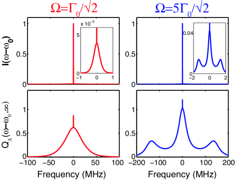
Figure 1: Predicted normalized line shape (top panes) and $Q_{\Delta}(\omega-\omega_{0},t=\infty)$ (bottom panes) for a 2-level dye with $\Gamma_{0}/2\pi=40MHz$ and two different Rabi frequencies $\Omega$ as indicated. $\Delta=0.2\;\mathrm{MHz}$. Insets truncate the y-axis to fully display the lineshape outside the vicinity of the high coherent peak at $\omega=\omega_{0}$.

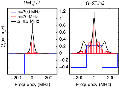
Figure 2: $Q_{\Delta}(\omega,t=\infty)$ for different values of $\Delta$ and the same cases as in fig. 1. The bar graph format is used to emphasize the size of and location of the frequency bins, but is absent at the finest discretization for clarity.

A traditional measure of broadband photon statistics is Mandel’s Q parameter Mandel (1979), which is defined as the ratio of the second factorial cumulant of $N_{(\omega,\infty)}(t)\equiv N(t)$ to the first factorial cumulant (i.e the average) of $N(t)$. $Q\left(t\right)\equiv\left[\langle N^{2}(t)\rangle-\langle N(t)\rangle^{2}-\langle N(t)\rangle\right]/\langle N(t)\rangle$. We introduce a generalization of this quantity appropriate to photon counting within a finite size frequency window

$$Q_{\Delta}(\omega,t) = \frac{\langle N^{(2)}_{(\omega,\Delta)}(t)\rangle-\langle N_{(\omega,\Delta)}(t)\rangle^{2}}{\langle N_{(\omega,\Delta)}(t)\rangle}$$

$$= \frac{\langle N^{2}_{(\omega,\Delta)}(t)\rangle-\langle N_{(\omega,\Delta)}(t)\rangle^{2}-\langle N_{(\omega,\Delta)}(t)\rangle}{\langle N_{(\omega,\Delta)}(t)\rangle}$$

and $Q_{\infty}\left(\omega,t\right)=Q\left(t\right)$. Fig. 1 plots both the emission lineshape (with finite resolution) $I(\omega-\omega_{0})\equiv\lim_{t\rightarrow\infty}\frac{d}{dt}\langle N_{(\omega,\Delta)}(t)\rangle$ and $Q_{\Delta}(\omega,\infty)$ for resonant excitation conditions $(\omega_{L}=\omega_{0})$ and $\Delta=\Gamma_{0}/400\pi=0.2\;\mathrm{MHz}$. Two different values of the Rabi frequency are considered: $\Omega=\Gamma_{0}/\sqrt{2}$ and $\Omega=5\Gamma_{0}/\sqrt{2}$. The effect of frequency binning is barely discernible in the lineshape when $\Delta$ is chosen so small. Our results are essentially identical to the classical emission spectrum of Mollow Mollow (1969), excepting the delta function “coherent” Mollow (1969); Cohen-Tannoudji et al. (1992) contribution at $\omega=\omega_{L}$, which adopts a finite height after frequency binning. Plots for $Q_{\Delta}\left(\omega,\infty\right)$ have not been reported previously, and at first sight our results appear surprising. The values selected for $\Omega$ in the chosen examples both yield sizable negative values for the traditional broadband $Q$ parameter ($-3/4$ and $-0.11$ for $\Omega=\Gamma_{0}/\sqrt{2}$ and $\Omega=5\Gamma_{0}/\sqrt{2}$ respectively), however $Q_{\Delta}(\omega,\infty)$ is seen to be positive over the entire frequency axis. The implication is that the antibunching phenomenon associated with $Q<0$ is due to correlations between photons of different frequencies. To make this point more explicitly, we plot $Q_{\Delta}(\omega,\infty)$ for different choices of $\Delta$ in fig. 2. $Q_{\Delta}(\omega,\infty)$ is seen to become negative over portions of the frequency axis as $\Delta$ approaches the width of the peaks in the spectrum. Related behavior has been predicted for the intensity correlation function ($g2$) of photons originating from a single well-resolved sideband in the Mollow triplet Aspect et al. (1980); Nienhuis (1993); Cohen-Tannoudji et al. (1992). In that case, antibunching may be explained via the allowed sequence of photon emissions in the radiative cascade predicted by the dressed atom picture Cohen-Tannoudji et al. (1992). Interestingly, narrowband bunching has previously been attributed to properties of the detector Nienhuis (1993), but we find the same effect in our observables that focus solely on photon emission.

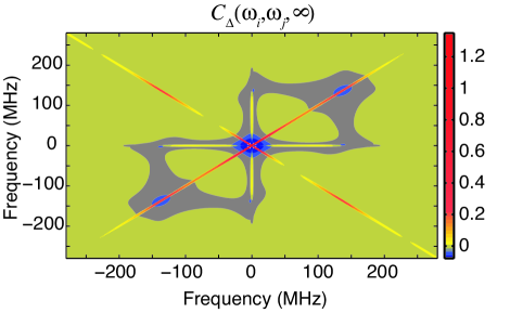
Figure 3: Contour plot of the normalized factorial covariance function (see eq. 11). We consider the $\Omega=5\Gamma/\sqrt{2}$ case of figs. 1 and 2 and have set $\Delta=2\;\mathrm{MHz}$.

Eq. 8 is easily generalized to calculate correlations between photons at different frequencies. We define a normalized photon covariance function as:

$$C_{\Delta}(\omega_{i},\omega_{j},t)=$$ (11)

$$\frac{\langle N_{(\omega_{i},\Delta)}(t)N_{(\omega_{j},\Delta)}(t)\rangle-\langle N_{(\omega_{i},\Delta)}(t)\rangle\langle N_{(\omega_{j},\Delta)}(t)\rangle}{\sqrt{\langle N_{(\omega_{i},\Delta)}(t)\rangle\langle N_{(\omega_{j},\Delta)}(t)\rangle}}-\delta_{\omega_{i},\omega_{j}}.$$

A discretized version of this correlation function in the limit $t\rightarrow\infty$ is plotted in fig. 3, where $\omega_{i(j)}$ have been chosen to follow $\omega_{i}=\omega_{0}+r\Delta$, where $r$ is any integer. When $\omega_{i}=\omega_{j}$, $C_{\Delta}(\omega_{i},\omega_{i},t)=Q_{\Delta}(\omega_{i},t)$. Otherwise, $C_{\Delta}(\omega_{i},\omega_{j},t)$ simply represents the covariance in photon number, normalized so as to give a finite result in the long time limit. Fig. 3 demonstrates that although $Q_{\Delta=\Gamma_{0}/40\pi}(\omega_{i},\infty)\geq 0$, the total $Q$ parameter is dominated by negative contributions from photons that are well separated in frequency; broadband measurement of $Q$ contains important contributions from correlations spanning the entire spectrally active region of the transition. The positive inter-sideband peaks in fig. 3 reflect the correlated emission of photons from opposite sidebands. This is in qualitative agreement with the inter-sideband bunching expected for a 2-level system excited far from resonance Aspect et al. (1980). The phenomenon is attributable to the necessary paring of photons from the two sidebands in order to maintain total energy conservation as photons of energy $\hbar\omega_{L}$ are absorbed by the molecule.

Our treatment of photon emission statistics is general and relies on no approximations beyond the RWA and Markov assumption for system dynamics. It is valid for arbitrary field strengths and does not assume particular physical regimes for the molecular system. Moreover, the present approach provides photon correlations between all possible frequency pairs, which enables calculation for any possible detector bandwidth and a quantitative demonstration of how seemingly inconsistent broadband versus narrowband statistics can arise from the same physical phenomena. This framework should prove valuable in the interpretation of future SMS experiments where moments higher than 1 will be measured and in understanding the molecular dynamics that such measurements probe. Several multi-state dye models are discussed in ref. Bel et al. (2006) and will be treated in a future study Bel and Brown .

This work was supported by the NSF (CHE-0349196). F. B. is an Alfred P. Sloan Research Fellow and a Camille Dreyfus Techer-Scholar.

References

- Moerner and Orrit (1999) W. E. Moerner and M. Orrit, Science 283, 1670 (1999). T. Plakhotnik, E. A. Donley, and U. P. Wild, Ann. Rev. Phys. Chem. 49, 181 (1997). X. S. Xie, J. Chem. Phys. 117, 11024 (2002). X. Zhuang et al, Science 288, 2048 (2000). S. Weiss, Science 283, 1676 (1999).
- Ha et al. (1996) T. Ha et al., Proc. Natl. Acad. Sci. U. S. A. 93, 6264 (1996).
- Moreau et al. (2001) E. Moreau et al., Phys. Rev. Lett 87, 183601 (2001).
- Luong et al. (2005) A. K. Luong et al., J. Phys. Chem. B 109, 15691 (2005).
- Jung et al. (2002) Y. Jung, E. Barkai, and R. J. Silbey, J. Chem. Phys. 117, 10980 (2002). E. Barkai, Y. J. Jung, and R. Silbey, Annual Review of Physical Chemistry 55, 457 (2004). M. Lippitz, F. Kulzer, and M. Orrit, ChemPhysChem 6, 770 (2005).
- Gopich and Szabo (2005) I. Gopich and A. Szabo, J. Chem. Phys. 122, 014707 (2005).
- Bel et al. (2006) G. Bel, Y. Zheng, and F. L. H. Brown, J. Phys. Chem. B 110, 19066 (2006).
- Aspect et al. (1980) A. Aspect et al., Phys. Rev. Lett. 45, 617 (1980).
- Nienhuis (1993) G. Nienhuis, Phys. Rev. A 47, 510 (1993).
- Cohen-Tannoudji et al. (1992) C. Cohen-Tannoudji, J. Dupont-Roc, and G. Grynberg, Atom-Photon Interactions (Wiley-Interscience, New York, 1992).
- Zheng and Brown (2003a) Y. Zheng and F. L. H. Brown, Phys. Rev. Lett. 90, 238305 (2003a). F. L. H. Brown, Accounts of Chemical Research 39, 363 (2006). Y. Zheng and F. L. H. Brown, J. Chem. Phys. 119, 11814 (2003b).
- Cook (1981) R. J. Cook, Phys. Rev. A 23, 1243 (1981). S. Mukamel, Phys. Rev. A 68, 063821 (2003).
- Wilcox (1967) R. M. Wilcox, J. Math. Phys. 8, 962 (1967).
- (14) We assume the electronic splitting far exceeds any nuclear energy scales in the system, and have replaced within the standard expression for with . Our assumptions (dipole operator completely non-diagonal in the electronic space and large electronic splitting) insure that for all relevant photons.
- (15) G. Bel and F. L. H. Brown, in preparation.
- Mollow (1969) B. R. Mollow, Phys. Rev. 188, 1969 (1969).
- Mandel (1979) L. Mandel, Opt. Lett. 4, 205 (1979).
- Gardiner (1991) C. W. Gardiner, Quantum Noise (Springer-Verlag, Berlin, 1991), p. 155.
- MPI (1994) W. E. Moerner et. al., J. Phys. Chem. 98, 7382 (1994).
- Grove (1977) R. E. Grove et. al., Phys. Rev. A 15, 227 (1977).