Large isotope effect on $T_{c}$ in cuprates despite of a small electron-phonon coupling

Abstract

We calculate the isotope coefficients $\alpha$ and $\alpha^{\ast}$ for the superconducting critical temperature $T_{c}$ and the pseudogap temperature $T^{\ast}$ in a mean-field treatment of the $t$-$J$ model including phonons. The pseudogap phase is identified with the $d$-charge-density wave ($d$-CDW) phase in this model. Using the small electron-phonon coupling constant $\lambda_{d}\sim 0.02$ obtained previously in LDA calculations in YBa₂Cu₃O₇, $\alpha^{\ast}$ is negative but negligible small whereas $\alpha$ increases from about 0.03 at optimal doping to values around 1 at small dopings in agreement with the general trend observed in many cuprates. Using a simple phase fluctuation model where the $d$-CDW has only short-range correlations it is shown that the large increase of $\alpha$ at low dopings is rather universal and does not depend on the existence of sharp peaks in the density of states in the pseudogap state or on specific values of the phonon cutoff. It rather is caused by the large depletion of spectral weight at low frequencies by the $d$-CDW and thus should also occur in other realizations of the pseudogap.

I Introduction

An open and rather controversially discussed topic in high-$T_{c}$ superconductivity is the role played by phonons for the low-energy electronic properties and, in particular, the high transition temperatures $T_{c}$. A direct way to show the involvement of the lattice in electronic properties is the study of the isotope effect on $T_{c}$. Franck Experimentally, the corresponding isotope coefficient $\alpha$ is very small in high-$T_{c}$ cuprates near optimal doping but increases strongly in the underdoped region attaining values being comparable or even larger than those in conventional phonon-mediated superconductors. It is often argued that these large observed isotope effects in the underdoped region give direct evidence for a large electron-phonon coupling in the cuprates. Franck ; Keller ; Bornemann It even has been suggested that it is so large that Eliashberg theory breaks down and that non-adiabatic and polaronic features play an important role in these systems. Alexandrov ; Buss ; Alexandrov1 ; Jarrell Other approaches have suggested that large isotope effects may occur in the presence of a pseudogap. Williams ; Dahm

Below we show that the essential features of the isotope experiments on T_c can be explained within a mean-field approximation of the $t$-$J$ model Morse ; Hsu ; Cappelluti ; Benfatto using very small values for the electron-phonon coupling. The pure $t$-$J$ model exhibits in mean-field approximation a competition of $d$-wave superconductivity and a $d$-CDW with transition temperatures $T_{c}$ and $T^{\ast}$, respectively. The observed pseudogap can be identified with the $d$-CDW phase in this model. Cappelluti ; Chakravarty Whereas many experiments support the idea of two competing phases Tacon ; Lee ; Wen ; Kondo ; Yu ; Mook ; Liu the nature of the additional phase remains unclear and many proposals besides of the $d$-CDW have been considered. Norman Experiments suggest that its order parameter has $d$-wave symmetry like that of the superconducting phase. This favors an unconventional charge- or spin density wave state with internal $d$-wave symmetry rather than a conventional one with (anisotropic) $s$-wave symmetry. The $t$-$J$ model yields at large $N$ ($N$ is the number of spin components) such a $d$-CDW but its relevance for the physical case $N=2$, for instance in form of a phase without long-range but strong $d$-wave short-range order, remains unclear. Leung ; Macridin ; Oles

In section II we introduce our model, its phase diagram and numerical results for the competing superconducting and CDW order parameters, and the corresponding transition temperatures $T_{c}$ and $T^{\ast}$. We then add phonons assuming always that the electron-phonon interaction is very small so that they can be treated in the weak-coupling approximation. Explicit formulas for the isotope coefficients $\alpha$ and $\alpha^{\ast}$ related to $T_{c}$ and $T^{\ast}$ will be given. In section III we present numerical results for the doping dependence of $\alpha$ and $\alpha^{\ast}$. In section IV we extend our treatment by including off-diagonal fluctuations in the $d$-CDW state using the method of Refs. Lee1 ; Bartosch ; Kuchinskii . In this way the pseudogap phase is treated more realistically because the long-range order is removed and self-energy effects are included. Our conclusions are found in section V.

II Theoretical framework

We consider the $t$-$J$ model Ogata with the Hamiltonian $H$,

$$H=-t\sum_{\langle i,j\rangle,\sigma}c^{\dagger}_{i\sigma}c_{j\sigma}-t^{\prime}\sum_{\langle i,j\rangle^{\prime},\sigma}c^{\dagger}_{i\sigma}c_{j\sigma}$$

$$+\frac{J}{2}\sum_{\langle i,j\rangle}{\bf S}_{i}{\bf S}_{j}-\frac{1}{4}(J-2V_{C})\sum_{\langle i,j\rangle}n_{i}n_{j}.$$ (1)

$c^{\dagger}_{i\sigma},c_{i\sigma}$ are creation and annihilation operators, respectively, for electrons at site $i$ and spin projection $\sigma$ subject to the condition that double occupancies of sites are excluded. The sums include nearest neighbor $\langle i,j\rangle$ and next nearest neighbor $\langle i,j\rangle^{\prime}$ sites on a 2D square lattice, the corresponding hopping elements are $t$ and $t^{\prime}$, respectively. ${\bf S}_{i}$ and $n_{i}$ are spin and site occupation operators, $J$ the Heisenberg coupling constant, and $V_{C}$ a Coulomb interaction between nearest neighbors.

One way to obtain a mean-field approximation for $H$ is to introduce $N$ spin components in Eq. (1), scale the coupling constants as $t\rightarrow 2t/N$, $t^{\prime}\rightarrow 2t^{\prime}/N$, $J\rightarrow 2J/N$ etc., and to consider the large $N$ limit. comment As a result $t$ and $t^{\prime}$ are renormalized yielding the quasi-particle dispersion $\epsilon({\bf k})$. At the same time the fermionic operators can be treated as usual creation and annihilation operators. Explicitly, one obtains $\epsilon({\bf k})=-2(\delta t+rJ)(\cos(k_{x})+\cos(k_{y}))-4t^{\prime}\delta\cos(k_{x})\cos(k_{y})-\mu$, with $r=1/N_{c}\sum_{\bf q}\cos({q_{x}})f(\epsilon({\bf q}))$. $f$ is the Fermi function, $\delta$ the doping away from half-filling, and $\mu$ a renormalized chemical potential. Here and in the following we use the lattice constant $a$ of the square lattice as length unit. As previously discussed Cappelluti ; Greco the relevant order parameters for our mean-field treatment of the $t$-$J$ model is a CDW order parameter

$$\Phi({\bf k})=-\frac{i}{N_{c}}\sum_{\bf q}J({\bf k}-{\bf q})\langle c^{\dagger}_{{\bf q}\uparrow}c_{{\bf q}+{\bf Q}{\uparrow}}\rangle,$$ (2)

with $J({\bf k})=2J(\cos k_{x}+\cos k_{y})$, and a superconducting (SC) order parameter

$$\Delta({\bf k})=\frac{1}{N_{c}}\sum_{\bf q}(J({\bf k}-{\bf q})-V_{C}({\bf k}-{\bf q}))\langle c_{{\bf q}\uparrow}c_{{-\bf q}\downarrow}\rangle.$$ (3)

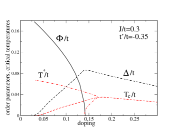
Figure 1: (Color online) Zero temperature order parameters $\Phi$ and $\Delta$ and the critical temperatures $T^{\star}$ and $T_{c}$ as a function of doping.

$N_{c}$ is the number of primitive cells, $\langle...\rangle$ denotes an expectation value, ${\bf Q}=(\pi,\pi)$ is the wave vector of the $d$-CDW, and $V_{C}({\bf k})=2V_{C}(\cos k_{x}+\cos k_{y})$. The Coulomb interaction $V_{C}({\bf k})$ between nearest neighbors has been introduced to prevent an instability of the $d$-CDW with respect to phase separation in some region of phase space. Cappelluti From the self-consistency condition for the self-energy one obtains coupled equations for $\Phi$, $\Delta$, the chemical potential and a renormalization contribution $r$ to the band dispersion due to $J$. Cappelluti ; Greco Their most stable solutions have $d$-wave symmetries in the interesting doping region, i.e., $\Phi({\bf k})=\Phi\gamma({\bf k})$ and $\Delta({\bf k})=\Delta\gamma({\bf k})$ with $\gamma({\bf k})=(\cos k_{x}-\cos k_{y})/2$.

A similar mean-field approximation as above is obtained by using a slave-boson representation for $H$ in Eq.(1), enforcing the constraint on the average, using usual mean-field decouplings for the third and fourth term in $H$, and dropping the antiferromagnetic order parameter. The above expression for $\epsilon({\bf k})$ as well as Eq.(3) are in this way exactly reproduced, Eq.(2) with $J/2+V_{C}$ instead of $J$.

Fig. 1 shows the doping dependence of $\Phi$ and $\Delta$ at zero temperature, calculated fully self-consistently for $t^{\prime}/t=-0.35$, $J/t=0.3$, and $V_{C}/J=0.2$. In the overdoped region $\delta\geq\delta_{c}\sim 0.14$ $\Phi$ is zero. In the underdoped region $\delta\leq\delta_{c}$ $\Phi$ is non-zero and coexists with $\Delta$. $\Delta$ shows a maximum near $\delta_{c}$ and decays approximately linearly in $\delta$ towards lower and higher dopings. The two order parameters compete with each other which causes the strong decay of $\Delta$ with decreasing doping in the underdoped region. Also shown in Fig. 1 is $T^{\star}$ (dash-dotted line) and $T_{c}$ (dashed line) where $\Phi$ and $\Delta$, respectively, vanish. $T^{\star}$ shows near $\delta_{c}$ a reentrant behavior which has a simple explanation: The piece of the $T^{\star}$ line above the $T_{c}$ curve is unaffected by superconductivity. Discarding superconductivity the $T^{\star}$ line would continue to the right decreasing slowly and reaching the $x$ axis only at around $\delta\sim 0.25$. Taking superconductivity into account $T^{\star}$ and also $\Phi$ are suppressed by the presence of a finite $\Delta$, i.e., below the $T_{c}$ curve. Since $\Delta$ increases rapidly with decreasing temperature $T^{\star}$ even bends back due to the strong repulsion and reaches the critical doping $\delta_{c}$ at zero temperature where $\Phi$ becomes nonzero. The reentrant behavior thus reflects the strong competition of the CDW and SC order parameters. The occurrence of a large coexistence region of $\Delta$ and $\Phi$, which extends down to $\delta=0$, is plausible because the Fermi surface consists in the $d$-CDW state of arcs around the nodal direction Greco which are unstable against the formation of a BCS gap $\Delta$.

In order to discuss the isotope effect we consider a phonon-induced electronic density-density coupling between nearest neighbors and on the same atom. Approximating its frequency dependence by a rectangular form, as is often done in approximate solutions of the Eliashberg equation,Carbotte this effective electron-electron interaction has in the $d$-wave channel the form,

$$v({\bf q},i\omega_{n})=-2Vn_{d}({\bf q},i\omega_{n})n_{d}({\bf-q},-i\omega_{n}),$$ (4)

$$n_{d}({\bf q},i\omega_{n})=\frac{1}{N_{c}}\sum_{{\bf k},\sigma=1,2}\gamma({\bf k})\Theta_{n}c^{\dagger}_{{\bf k}+{\bf q}{\sigma}}c_{{\bf k}{\sigma}}.$$ (5)

Similarly, we have in the isotropic $s$-wave channel,

$$w({\bf q},i\omega_{n})=-\frac{W}{2}n({\bf q},i\omega_{n})n({\bf-q},-i\omega_{n}),$$ (6)

$$n({\bf q},i\omega_{n})=\frac{1}{N_{c}}\sum_{{\bf k},\sigma=1,2}\Theta_{n}c^{\dagger}_{{\bf k}+{\bf q}{\sigma}}c_{{\bf k}{\sigma}}.$$ (7)

$V$ and $W$ are electron-phonon (EP) coupling constants in the $d$ and $s$-wave channels, respectively, $\Theta_{n}$ the cutoff function $\Theta(\omega_{D}-|\omega_{n}|)$, $\omega_{n}$ the bosonic Matsubara frequency $\omega_{n}=2n\pi T$, and $\omega_{D}$ the phonon cutoff frequency. $n_{d}({\bf q},i\omega_{n})$ and $n({\bf q},i\omega_{n})$ are electronic density operators with $d$ and $s$-wave symmetry, respectively. Effects due to a small EP interaction can be taken into account in the curves of Fig. 1 by adding the electronic self-energy due to $v({\bf q},i\omega_{n})$ and $w({\bf q},i\omega_{n})$ in the form of a Fock diagram. The resulting self-consistent equations lead to an equation for the renormalization function $Z({\bf k},i\omega_{n})$ due to $W$. At $T=T_{c}$ this equation can be solved directly yielding $Z({\bf k},i\omega_{n})\equiv Z=1+\lambda_{s}$ where $\lambda_{s}$ is the product of $W$ and the electronic density at the Fermi energy and $T=T_{c}$, i.e., it refers in general to the $d$-CDW state. A second equation is obtained which determines the SC order parameter $\Delta({\bf k},i\omega_{n})$,

$$\Delta({\bf k},i\omega_{n})=-4\tilde{J}\gamma({\bf k})\frac{T}{N_{c}}\sum_{{\bf k}^{\prime}n^{\prime}}\gamma({\bf k}^{\prime})g_{12}({\bf k}^{\prime},i\omega_{n^{\prime}})-$$

$$-4V\gamma({\bf k})\Theta_{n}\frac{T}{N_{c}}\sum_{{\bf k}^{\prime}n^{\prime}}\gamma({\bf k}^{\prime})\Theta_{n^{\prime}}g_{12}({\bf k}^{\prime},i\omega_{n^{\prime}}).$$ (8)

$\tilde{J}$ is equal to $J-V_{C}$. $g_{12}$ is the 12-element of the 4$\times$4 matrix Green’s function $g$. Its inverse $g^{-1}({\bf k},i\omega_{n})$ is given by,

$$\left(\begin{array}[]{c c c c}i\omega_{n}Z-\epsilon({\bf k})&-\Delta({\bf k},i\omega_{n})&-i\Phi({\bf k},i\omega_{n})&0\\ -\Delta({\bf k},i\omega_{n})&i\omega_{n}Z+\epsilon({\bf k})&0&i\Phi({\bf\bar{k}},i\omega_{n})\\ i\Phi({\bf k},i\omega_{n})&0&i\omega_{n}Z-\epsilon({\bf\bar{k}})&-\Delta({\bf\bar{k}},i\omega_{n})\\ 0&-i\Phi({\bf\bar{k}},i\omega_{n})&-\Delta({\bf\bar{k}},i\omega_{n})&i\omega_{n}Z+\epsilon({\bf\bar{k}})\end{array}\right)$$ (9)

with the abbreviation $\bf{\bar{k}}={\bf k-Q}$. $\Phi({\bf k},i\omega_{n})$ is the $d$-CDW order parameter renormalized by the phonons and given by,

$$i\Phi({\bf k},i\omega_{n})=-4J\gamma({\bf k})\frac{T}{N_{c}}\sum_{{\bf k^{\prime}}n^{\prime}}\gamma({\bf k^{\prime}})g_{13}({\bf k^{\prime}},i\omega_{n^{\prime}})$$

$$+2V\gamma({\bf k})\Theta_{n}\frac{T}{N_{c}}\sum_{{\bf k^{\prime}}n^{\prime}}\Theta_{n^{\prime}}\gamma({\bf k^{\prime}})g_{13}({\bf k^{\prime}},i\omega_{n^{\prime}}),$$ (10)

where $g_{13}$ is the 13-element of the Green’s function matrix $g$.

For the calculation of $T_{c}$ it is sufficient to linearize the right-hand side of Eq. (8) with respect to $\Delta({\bf k},i\omega_{n})$. Furthermore, we may neglect the phonon renormalization for $\Phi$ in this case: Below we will be interested only in a small EP constant $V$ yielding also only a small renormalization. Moreover, as will be shown below, this small renormalization is practically independent of the ionic mass $M$ and thus may be neglected in calculating the isotope effect on $T_{c}$. We therefore have solved Eq. (10) using only the first term on the right-hand side and use the solution in Eq. (9) to obtain $g_{12}$. Eq. (8) represents an integral equation with two separable kernels which can easily be solved. Writing Eq.(8) as a condition for $T_{c}$ we find,

$$(1+F_{11})(1+F_{22})-F_{12}^{2}=0,$$ (11)

with

$$F_{11}=-2{\tilde{J}}\int_{0}^{\infty}d\omega\frac{N_{d}(Z\omega)}{Z\omega}tanh(\frac{\omega}{2T_{c}}),$$ (12)

$$F_{12}=-2\sqrt{V{\tilde{J}}}\int_{0}^{\infty}d\omega\frac{N_{d}(Z\omega)}{Z\omega}\frac{2}{\pi}\Im[\psi(\frac{1}{2}+{\frac{i\omega}{2\pi T_{c}}})$$

$$-\psi({\frac{\omega_{D}}{2\pi T_{c}}}+1+{\frac{i\omega}{2\pi T_{c}}})],$$ (13)

and $F_{22}=\sqrt{V/{\tilde{J}}}F_{12}$. $\psi$ is the digamma function and $\Im$ denotes the imaginary part. $N_{d}({\omega})$ is given by

$$N_{d}(\omega)=\frac{2\omega}{\pi N_{c}}\sum_{\bf k}\gamma^{2}({\bf k})\Im[G({\bf k},\omega-i\eta)],$$ (14)

where $\eta$ is a positive infinitesimal quantity,

$$G({\bf k},z)=\frac{z^{2}-\epsilon^{2}({\bf\bar{k}})-\Phi^{2}({\bf k})}{(z^{2}-\lambda_{1}^{2}({\bf k}))(z^{2}-\lambda_{2}^{2}({\bf k}))},$$ (15)

and

$$\lambda_{1,2}=\frac{\epsilon({\bf k})+\epsilon({\bf\bar{k}})}{2}\pm\frac{1}{2}\sqrt{(\epsilon({\bf k})-\epsilon({\bf\bar{k}}))^{2}+4\Phi^{2}({\bf k})}.$$ (16)

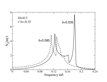
Figure 2: Weighted density $N_{d}(\omega)$ of electronic states for two dopings $\delta$.

$N_{d}(\omega)$ represents a weighted density of electronic states at $T_{c}$ and is shown in Fig. 2 for two different dopings. It consists of a sharp peak near the energy $\Phi$ due to excitations across the $d$-CDW gap and a structure at lower energies related to the van Hove singularity. It is convenient to characterize $V$ by a dimensionless EP coupling constant,

$$\lambda_{d}=VN_{d}(0).$$ (17)

According to the above equations phonons affect $T_{c}$ in a two-fold way, namely, via $V=\lambda_{d}/N_{d}(0)$ and via $Z=1+\lambda_{s}$. $\lambda_{d}$ and $\lambda_{s}$ characterize the phonon-induced pairing interaction of $d$-wave and $s$-wave symmetry, respectively. Putting $\lambda_{s}$ to zero $V$ increases $T_{c}$. To see this we rewrite Eq. (11) in the form $1+\hat{F}_{11}=0$. $\hat{F}_{11}$ is given by Eq. (12) if one makes there the change ${\tilde{J}}\rightarrow{\tilde{J}}/(1-F_{12}^{2}/(1+F_{22}))$. This means that $V$ increases ${\tilde{J}}$ and thus increases $T_{c}$. On the other hand, if we put $V=0$ Eq. (11) reduces to $1+\hat{F}_{11}=0$ with $\hat{F}_{11}$ given by Eq. (12) modified by ${\tilde{J}}\rightarrow{\tilde{J}}/Z$ and $T_{c}\rightarrow T_{c}Z$. Each of these two changes diminishes $T_{c}$. Thus phonons may lower or may increase $T_{c}$ depending which of the above two effects is larger. Numerical calculations indicate that generically the second effect dominates and that $T_{c}$ decreases if one couples to phonons. Macridin1 Most important for us is, however, the following observation. Our aim is not to determine the change in $T_{c}$ when the electron-phonon coupling is turned on but when the ionic mass $M$ is changed. It is well known that $\lambda_{s}$ is independent of the ionic mass $M$, thus there will be no change in $Z$ by isotope substitutions and $\alpha$ will always be positive. For small EP couplings we may even put $Z=1$ and keep only the linear term in $V$ in the calculation of the isotope coefficient $\alpha=-d\ln T_{c}/d\ln M$. From Eq. (11) one finds for $\alpha$ in this limit,

$$\alpha=\frac{\omega_{D}}{T_{c}}F_{12}\Bigl{(}\frac{\partial F_{12}}{\partial\omega_{D}}\Bigr{)}\Bigl{(}\frac{\partial F_{11}}{\partial T_{c}}\Bigr{)}^{-1},$$ (18)

where the derivatives in Eq. (18) are to be taken at the $T_{c}$ without phonons and we also assumed $\omega_{D}\sim M^{-0.5}$.

III Results for the isotope coefficients

In deriving the above formulas we assumed that the phonon-induced interaction $V$ affects only $\Delta$ but not $\Phi$ and thus also not $T^{\ast}$. To check this approximation we have calculated the isotope coefficient $\alpha^{\star}$ related to $T^{\star}$ and defined by $\alpha^{\ast}=-d\ln T^{\ast}/d\ln M$. The calculation of $\alpha^{\ast}$ is very similar to that of $\alpha$.

Table 1: Isotope coefficient $\alpha^{\ast}$ for different dopings $\delta$

$\delta$	0.028	0.048	0.064	0.090	0.115	0.139	0.164
$100\cdot\alpha^{\ast}$	$-0.20$	$-0.24$	$-0.27$	$-0.34$	$-0.42$	$-0.53$	$-0.66$

Numerical values for $\alpha^{\ast}$ as a function of doping throughout the underdoped regime are given in TABLE I for $V/t=0.04$ and $\omega_{D}/t=0.1$. All values for $\alpha^{\ast}$ are negative, i.e., $\alpha^{\ast}$ shows an inverse isotope effect. However, this isotope effect is two orders of magnitude smaller than the usual BCS value of 1/2 and thus tiny. Furthermore, the absolute value of $\alpha^{\ast}$ decreases with decreasing doping quite in contrast to $\alpha$ as will be shown below. The negligible isotope effect on $T^{\ast}$ which we found is in agreement with the experiment Williams though there exist also data which have been interpreted in terms of a large isotope coefficient $\alpha^{\ast}$. Rubio Strictly speaking in our calculation of $\alpha$ the renormalized $d$-CDW order parameter at $T=T_{c}$ enters the density of states function $N_{d}(\omega)$, Eq. (12). Since we have shown that $T^{\ast}$ is independent of the ionic mass $M$ we may conclude that the $d$-CDW order parameter at $T=T_{c}$ has also only a negligible isotope effect justifying the above procedure to calculate $\alpha$.

Fig. 3 shows $\alpha$ as a function of doping for $V/t=0.04$ and two phonon cutoffs $\omega_{D}$ corresponding to the buckling and half-breathing phonon modes in YBa₂Cu₃O₇. Pintschovius In the overdoped region $\alpha$ is nearly independent of $\omega_{D}$ and $\delta$ and about 0.03, i.e., very small. In the underdoped region $\alpha$ monotonically increases with decreasing $\delta$ and reaches appreciable values, for instance, 1/4 at a $T_{c}$ which is only reduced by a factor 2 from its maximum value.

To understand the increase of $\alpha$ at low dopings better one can rewrite Eq. (18) approximately as $\langle N_{d}(\omega)\rangle/N_{d}(0)(-F_{22})$, using a low $T_{c}$ approximation in the denominator.

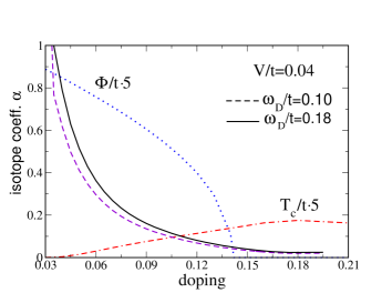
Figure 3: (Color online) Isotope coefficient $\alpha$ as a function of doping for two phonon cutoffs $\omega_{D}$. Also shown are the curves for $\Phi$ and $T_{c}$ from Fig. 1

.

$\langle N_{d}(\omega)\rangle$ is an average of $N_{d}(\omega)$ around the phonon frequency $\omega_{D}$ over an energy interval of about $\omega_{D}$. This interval is determined by the functions $\psi$ in Eq. (13) and caused by the sharp cutoff in Matsubara frequencies. According to Fig. 2 $N_{d}(0)$ decreases rapidly with decreasing $\delta$ reflecting the fact that $N_{d}(0)$ is due to the arcs left over from the Fermi line after formation of the $d$-CDW gap. The length of the arcs, however, decreases strongly with decreasing $\delta$. From Fig. 2 it is clear that for most phonon frequencies the large spectral weight near the $d$-CDW gap will substantially contribute to this average. As a result $\langle N_{d}(\omega)\rangle/N_{d}(0)\gg 1$ and, since $-F_{22}$ is a slowly increasing function with decreasing $\delta$, a large enhancement of $\alpha$ results at low dopings. A sharp cutoff for real frequencies, usually used in BCS-theory, would yield $\langle N_{d}(\omega)\rangle=N_{d}(\omega_{D})$. Consequently $\alpha$ would exhibit strong resonances for $\omega_{D}\sim\Phi$ or, more generally, if $\omega_{D}$ is near well-pronounced peaks in $N_{d}(\omega)$. Implementing the phonon cutoff in terms of Matsubara frequencies, as we did, corresponds to a rather soft cutoff in real frequencies. Such a procedure is closer to an exact solution of Eliashberg equations, yields a finite phonon contribution to $Z$ and is also free of the above unphysical resonances in $\alpha$ if $\omega_{D}$ and the gap energy $\Phi$ are of similar magnitude. Another advantage of our procedure is that $\alpha$ depends only weakly on $\omega_{D}$, also for $\delta\leq\delta_{c}$. If there is no pseudogap $N_{d}(\omega)$ is rather constant in the phonon energy region which means that the above density ratio $\langle N_{d}(\omega)\rangle/N_{d}(0)$ is one and $\alpha$ very small for all dopings.

Qualitatively, the curves for $\alpha$ in Fig. 3 are similar to those in Refs. Williams ; Dahm where phenomenological pseudogaps were used and the problem of resonances was avoided either by considering only the limit $\omega_{D}\gg\Phi$ or by a non-states-conserving pseudogap. This as well as the above approximate expression for $\alpha$ in terms of the density ratio $\langle N_{d}(\omega)\rangle/N_{d}(0)$ suggests that the above curves for $\alpha$ are rather independent of the specific features of our model ($d$-CDW with long-range order) but rather generic for underdoped cuprates with a pseudogap.

Very remarkable in Fig. 3 is the fact that the tiny value of 0.04 for the effective EP coupling $V/t$ is able to produce large values for $\alpha$ comparable to those seen in experiment in the underdoped region. The LDA yields $\lambda_{d}\sim 0.022$ in YBa₂Cu₃O₇, Heid which is roughly one order of magnitude smaller than $\lambda_{s}$. Heid1 ; Cohen (For a different view on the magnitude of the EP coupling constants in cuprates, see Ref. Reznik ). Using the LDA value $N_{d}(0)=1.108/eV$ from Ref. Heid , the relation Eq.(17) and $t=0.5eV$ we get in the LDA $V/t\sim 0.04$ which is the value used in our calculation. This shows that the large experimental values for $\alpha$ in the underdoped region do not contradict, at least in our competing model, the small LDA values for the EP coupling. The case of overdoped samples is presently less clear because of conflicting experimental results. Franck ; Pringle An isotope coefficient $\alpha$ which is small throughout the overdoped region Pringle would agree with our Fig. 3.

IV Extension to finite correlation lengths of the $d$-CDW

In the previous sections our employed mean field treatment yielded a $d$-CDW with long-range order and excitations with infinite long lifetimes. Such idealizations are certainly not realized in the cuprates and one may wonder to what degree our previous results depend on them. Generally speaking we do not expect drastic modifications because the strong increase of $\alpha$ with decreasing doping was due to the rearrangement of spectral weight due to the $d$-CDW gap. This shift of spectral weight should not be seriously affected by fluctuations or the loss of long-range order as long as the correlation length is sufficiently large. In this section we will investigate this expectation on a more quantitative level. To this end we will employ a modelLee1 ; Bartosch ; Kuchinskii which allows to treat exactly a certain class of semiclassical fluctuations of the off-diagonal order parameter.

First we consider only the $d$-CDW part of $g^{-1}$, i.e., the first and third rows and columns of Eq.(9) where we may put $Z=1$ considering again the weak-coupling case. Transforming the part induced by the variation of the order parameter into $\bf r$-space we get,

$$g_{CDW}^{-1}({\bf k}-i\nabla,i\omega_{n})=$$

$$\left(\begin{array}[]{c c }i\omega_{n}-\epsilon({\bf k}-i\nabla)&-i\gamma({\bf k})\Phi_{0}e^{i\beta}\\ i\gamma({\bf k})\Phi_{0}e^{-i\beta}&i\omega_{n}-\epsilon({\bf\bar{k}}-i\nabla)\end{array}\right),$$ (21)

with $\beta={\bf p}{\bf x}+\phi$ and ${\bf{\bar{k}}}={\bf k}-{\bf Q}$. ${\bf p}$ is a random variable with cartesian components distributed according to a Lorentzian. $\phi$ is a random phase which will not enter our final expressions and thus its distribution function has not to be specified. We apply now the unitary transformation

$$U_{1}({\bf x})=e^{i\beta\sigma_{3}/2},$$ (22)

to Eq.(21), where $\sigma_{3}$ is a Pauli matrix. After some algebra we find,

$$\tilde{g}_{CDW}^{-1} ( {\bf k}-i\nabla,i\omega_{n})=U^{\dagger}_{1}({\bf x})g_{CDW}^{-1}({\bf k}-i\nabla,i\omega_{n})U_{1}({\bf x})$$ (25)

$$= \left(\begin{array}[]{c c }i\omega_{n}-\epsilon({\bf k})+\epsilon_{1}&-i\gamma({\bf k})\Phi_{0}\\ i\gamma({\bf k})\Phi_{0}&i\omega_{n}-\epsilon({\bf\bar{k}})+\epsilon_{2}\end{array}\right),$$

with the abbreviations $\epsilon_{1}={\bf v}({\bf k}){\bf p}/2$ and $\epsilon_{2}=-{\bf v}({\bf{\bar{k}}}){\bf p}/2$. $v_{x,y}({\bf k})$ are given by $\partial\epsilon({\bf k})/\partial{k_{x,y}}$. In deriving Eq.(LABEL:matrix2) we also expanded $\epsilon({\bf k}-i\nabla)$ up to first order in $\nabla$ assuming that the changes in one-particle energies induced by the variation of the order parameter vary slowly in space. To simplify the following we will take $\epsilon_{1}=\epsilon_{2}=\epsilon$ which holds exactly for the case $t^{\prime}=0$.

The matrix in Eq.(LABEL:matrix2) can be diagonalized by a second unitary transformation $U_{2}$ yielding,

$$U_{2}^{\dagger}({\bf k})\tilde{g}_{CDW}^{-1}({\bf k},i\omega_{n})U_{2}({\bf k})=$$

$$\left(\begin{array}[]{c c }i\omega_{n}-\lambda_{1}({\bf k})+\epsilon&0\\ 0&i\omega_{n}-\lambda_{2}({\bf k})+\epsilon\end{array}\right),$$ (29)

with the eigenvalues $\lambda_{1,2}({\bf k})$ of the unperturbed $d$-CDW, given by Eq.(16). Taking also superconductivity into account we note that the Heisenberg interaction is invariant under the gauge transformation $U_{1}$. Applying the second unitary transformation $U_{2}$ to the Heisenberg interaction and using the BCS factorization the transformed matrix $g^{-1}$ splits into two 2x2 matrices and the resulting gap equation can easily be calculated. Adding also phonons one finds that Eqs.(11)-(13) still hold if the density $N_{d}(\omega)$ of Eq.(14) is replaced by the expression,

$$\frac{\omega}{\pi N_{c}}\sum_{{\bf k},\beta}\gamma({\bf k})^{2}\Im\frac{1}{(\omega-i\eta+\epsilon)^{2}-\lambda_{\beta}^{2}({\bf k})}.$$ (30)

Finally,

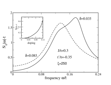
Figure 4: Weighted density of electronic states $\bar{N}_{d}(\omega)$ for two dopings $\delta$ for a correlation length $\xi=250$. The inset shows $\bar{N}_{d}(0)$ at low dopings.

Eqs.(11)-(13) have to be averaged over the distribution function $P({\bf p})$,

$$P({\bf p})=\frac{\kappa^{2}}{\pi^{2}(p_{x}^{2}+\kappa^{2})(p_{y}^{2}+\kappa^{2})},$$ (31)

where $\kappa=1/\xi$ and $\xi$ is the correlation length of the off-diagonal order parameter fluctuations. According to Eq.(21) $\Phi_{0}$ is the equilibrium $d$-CDW order parameter after omitting the factor $\gamma({\bf k})$. It thus varies in $\bf r$-space with the momentum $\bf Q$ because it connects electron states with momenta $\bf k$ and $\bar{\bf k}$. The random variable $\bf p$ modulates the equilibrium total momentum $\bf Q$ of the $d$-CDW in an additive way and it is distributed according to a Lorentzian. It is sufficient to apply the necessary average over $\bf p$ just to the expression of Eq.(30) yielding,

$$\bar{N}_{d}(\omega)=\frac{\omega}{\pi N_{c}}\sum_{{\bf k},\beta}\gamma({\bf k})^{2}$$

$$\Im\frac{1}{(\omega-i/(2\xi)(|v_{x}({\bf k})|+|v_{y}({\bf k})|))^{2}-\lambda_{\beta}^{2}({\bf k})}.$$ (32)

It is easy to see that the above expression can formally be obtained from $N_{d}(\omega)$ if one replaces there the infinitesimal $\eta$ by the finite, $\bf k$-dependent imaginary part $(|v_{x}({\bf k})|+|v_{y}({\bf k})|)/(2\xi)$. The latter quantity is in Eq.(32) averaged over the Fermi line in the pure $d$-CDW state, i.e., for $\beta=1$ over the arc around the nodal line and for $\beta=2$ over the remaining small piece near the antinodal point which however, vanishes for our two considered dopings. Thus the $\beta=2$ contribution in Eq.(32) is negligible small. In the $\beta=1$ contribution $(|v_{x}({\bf k})|+|v_{y}({\bf k})|)/(2\xi)$ varies only little along the arc so we may replace this quantity by its average over the arc and obtain for $\delta=0.085$ the value $1.15v_{F}/\xi$ where $v_{F}\sim 4.6t$ is the square root of the Fermi surface average of ${\bf v}^{2}({\bf k})$ in the normal state. This allows to describe phase correlations with a finite correlation length $\xi$ as an inverse life time effect with energy $\Gamma/t=1.15v_{F}/(t\xi)$.

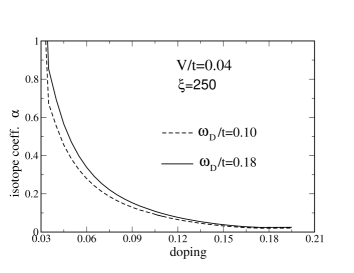
Figure 5: Isotope coefficient $\alpha$ as a function of doping for two phonon cutoffs $\omega_{D}$ calculated in the presence of short-ranged correlated phase fluctuations with correlation length $\xi=250$.

Fig. 4 shows $\bar{N}_{d}(\omega)$ for the two dopings of Fig. 2 and for the case of a correlation length $\xi=250$, corresponding to an inverse lifetime of about $0.02t$. Though such a large correlation length may seem to simulate a rather well-ordered state most of the fine structures in Fig. 2 are wiped out by phase fluctuations. In particular, the two peaks seen in Fig. 2 have merged into one broad and rather structureless peak. At low frequencies the changes introduced by phase fluctuations are rather minor. In the inset in Fig. 4 the static value $\bar{N}_{d}(0)$ is plotted as a function of doping showing the pronounced decrease of $\bar{N}_{d}(0)$ with decreasing $\delta$ similar as in the case without phase fluctuations in Fig. 2. This behavior for the density is rather robust as function of $\xi$ as long as $\xi\gg 1$ holds.

Fig. 5 shows the doping dependence of the isotope coefficient $\alpha$ using the same parameter as in Fig. 3 but $\bar{N}_{d}(\omega)$ instead of $N_{d}(\omega)$. Comparing Figs. 3 and 5 reveals that this change of densities does hardly affects $\alpha$ so that corresponding curves in these two figures are practically identical. This demonstrates that the steep increase of $\alpha$ with decreasing doping is not related or even caused by the sharp peaks present in $N_{d}(\omega)$ or by special values for the phonon cutoff $\omega_{D}$. Instead, it is a rather universal property caused by the large shift of spectral weight towards higher frequency due to the pseudogap. If the correlation length $\xi$ is decreased from large to small values of the order of the lattice constant the depletion in the density $\bar{N}_{d}(0)$ at low energies becomes smaller and smaller. In accordance with the decreasing shift of spectral weight from low to high energies the isotope coefficient $\alpha$ also decreases approaching a similar small value as in the absence of a pseudogap, i.e., in the overdoped region.

Fig. 5 can qualitatively be understood in a simple way considering our previously approximate expression $\langle N_{d}(\omega)\rangle/{N_{d}(0)}$ for $\alpha$. The numerator is essentially given by the area under the density curve in Figs. 2 and 4. Its value thus is independent of the shape of the density curve, i.e., whether it has sharp or broad peaks, as long as the area below the curve is constant. This area is practically the same in Figs. 2 and 4. On the other hand the $\omega=0$ values of the densities both decrease strongly and in a similar way with decreasing $\delta$. As a result $\alpha$ should be of similar magnitude in both cases and, in particular, show a strong increase towards low dopings in agreement with Fig. 5. The above approximate expression for $\alpha$ may also explain why the calculated values for $\alpha$ of Ref. Jarrell are for our electron-phonon coupling $V$ much smaller than ours: Their density of state function at $\lambda_{d}=0$, plotted in their Fig. 4, is large at $\omega=0$ compared to the modulation due to the pseudogap which implies only a small redistribution of spectral weight by the pseudogap.

V Conclusions

We have shown that a mean-field treatment of the $t$-$J$ model which identifies the pseudogap with the gap of a $d$-CDW state is able to explain the large isotope effect in underdoped cuprates. Interestingly, a very small EP coupling constant $V/t\sim 0.04$ is sufficient to explain the experimental data. This value is very close to that calculated for YBa₂Cu₃O₇ within the LDA. This shows that the large values for $\alpha$ of order 1 found in the underdoped region are, at least in our competing model, compatible with the small EP coupling constants predicted by the LDA. The obtained huge increase of the isotope coefficient $\alpha$ with decreasing doping is rather independent of the phonon cutoff frequency $\omega_{D}$ and the spectral properties of the excitations in the pseudogap state. The latter information is obtained by considering a simple phase fluctuation model where the $d$-CDW state has only short-range correlations.

Most important for the large increase of $\alpha$ with decreasing doping is in our calculation the large depletion of spectral weight at low frequencies and its shift to high energies by the pseudogap. Because of this we conjecture that our results are not specific to the employed $d$-CDW providing the pseudogap but also hold for other order parameters such as the antiferromagnet order parameter as long as they lead to a strong depletion of spectral weight at low frequencies. Our calculation shows, in particular, that it is not necessary to assume a large EP interaction in cuprates or extrinsic effects such as pairbreaking due to impurities Tallon ; Bill to explain the observed isotope effect of $T_{c}$.

The authors thank O. Gunnarsson for discussions and A.M. Oleś for a critical reading of the manuscript.

References

- (1) J.P. Franck, in Physical Properties of High Temperature Superconductors IV, edited by D.M. Ginsberg (World Scientific, Singapore, 1994), p. 189, and references therein.
- (2) H. Keller, Superconductivity in Complex Systems, Structure and Bonding (Springer-Verlag, Berlin, 2005), Vol. 114, p. 143.
- (3) H.J. Bornemann and D.E. Morris, Phys. Rev. B 44, 5322 (1991).
- (4) P.E. Kornilovitch and A.S. Alexandrov, Phys. Rev. B 70, 224511 (2004) and references therein.
- (5) A. Macridin and M. Jarrell, Phys. Rev. B 79, 104517 (2009).
- (6) A. Bussmann-Holder, H. Keller, A. R. Bishop, A. Simon, R. Micnas, and K. A. Müller, Europh. Lett. 72, 423 (2005).
- (7) A.S. Alexandrov and G.M. Zhao, arXiv:0807.3856.
- (8) G. V. M. Williams, J. L. Tallon, J. W. Quilty, H. J. Trodahl, and N. E. Flower, Phys. Rev. Lett. 80, 377 (1998).
- (9) T. Dahm, Phys. Rev. B 61, 6381 (2000).
- (10) D.C. Morse and T.C. Lubensky, Phys. Rev. B 43, 10436 (1991).
- (11) T.C. Hsu, J.B. Marston, and I. Affleck, Phys. Rev. B 43, 2866 (1991).
- (12) E. Cappelluti and R. Zeyher, Phys. Rev. B 59, 6475 (1999).
- (13) L. Benfatto, S. Caprara, C. Di Castro, Eur. Phys. J B17, 95 (2000).
- (14) S. Chakravarty, R.B. Laughlin, D.K. Morr, and C. Nayak, Phys. Rev. B 63, 94503 (2001).
- (15) M. Le Tacon, A. Sacuto, A. Georges, G. Kotliar, Y. Gallais, D. Colson, and A. Forget, Nature Physics 2, 537 (2006).
- (16) W. S. Lee, I. M. Vishik, K. Tanaka, D. H. Lu, T. Sasagawa, N. Nagaosa, T. P. Devereaux, Z. Hussain, and Z.-X. Shen, Nature 450, 81 (2007).
- (17) Hai-Hu Wen and Xiao-Gang Wen, Physica C 460, 28 (2007).
- (18) Takeshi Kondo, Tsunehiro Takeuchi, Adam Kaminski, Syunsuke Tsuda, and Shik Shin, Phys. Rev. Lett. 98, 267004 (2007).
- (19) Li Yu, D. Munzar, A. V. Boris, P. Yordanov, J. Chaloupka, Th. Wolf, C. T. Lin, B. Keimer, and C. Bernhard, Phys. Rev. Lett. 100, 177004 (2008).
- (20) H. A. Mook, Y. Sidis, B. Fauqu, V. Baldent, and P. Bourges, Phys. Rev. B 78, 020506(R) (2008).
- (21) Y. H. Liu, Y. Toda, K. Shimatake, N. Momono, M. Oda, and M. Ido, Phys. Rev. Lett. 101, 137003 (2008).
- (22) M.R. Norman, D. Pines and C. Kallin, Adv. Phys. 54, 715 (2005).
- (23) P.W. Leung, Phys. Rev. B 62, R6112 (2000), Phys. Rev. B 63, 94503 (2001).
- (24) A. Macridin, M. Jarrell, and Th. Maier, Phys. Rev. B 70, 113105 (2004).
- (25) M. Raczkowski, D. Poilblanc, R. Frésard, and A.M. Oleś, Phys. Rev. B 75, 094505 (2007).
- (26) P.A. Lee, T.M. Rice, and P.W. Anderson, Phys. Rev. Lett. 31, 462 (1973).
- (27) L. Bartosch and P. Kopietz, Eur. J. Phys. B 17, 555 (2000).
- (28) E.Z. Kuchinskii, M.V. Sadovskii, JETP 94, 654 (2002).
- (29) For a recent review, see M. Ogata and H. Fukuyama, Rep. Prog. Phys. 71, 036501 (2008).
- (30) In most treatments, for instance in Refs. Grilli ; Greco , the prefactor 2 in the scaling of coupling constants is omitted. The physical Hamiltonian is thus for reproduced only with an overall prefactor 1/2 causing additional prefactors of 1/2 in front of every coupling constant in subsequent equations.
- (31) M. Grilli and G. Kotliar, Phys. Rev. Lett. 64, 1170 (1990).
- (32) A. Greco and R. Zeyher, Phys. Rev. B 70, 024518 (2004).
- (33) J.P. Carbotte, Rev. of Mod. Physics 62, 1027 (1990).
- (34) A. Macridin, B. Moritz, M. Jarrell, and T. Maier, Phys. Rev. Lett. 97, 056402 (2006).
- (35) D. Rubio Temprano, K. Conder, A. Furrer, H. Mutka, V. Trounov, and K. A. Müller, Phys. Rev. B 66, 184506 (2002).
- (36) L. Pintschovius, physica status solidi (b) 242, 30 (2005).
- (37) R. Heid, R. Zeyher, D. Manske, and K.-P. Bohnen, Phys. Rev. B 80, 024507 (2009).
- (38) R. Heid, K.-P. Bohnen, R. Zeyher, and D. Manske, Phys. Rev. Lett. 100, 137001 (2008).
- (39) F. Giustino, M.L. Cohen and S.G. Louie, Nature 452, 975 (2008).
- (40) D. Reznik, G. Sangiovanni, O. Gunnarsson, and T.P. Devereaux, Nature 455, E6 (2008).
- (41) D.J. Pringle, G.V.M. Williams, and J.L. Tallon, Phys. Rev. B 62, 12527 (2000).
- (42) J.L. Tallon, R.S. Islam, J. Storey, G.V.M. Williams, and J.R. Cooper, Phys. Rev. Lett. 94, 237002 (2005).
- (43) A. Bill, V.Z. Kresin, and S.A. Wolf, in Pair Correlations in Many-Body Systems, ed. by V.Z. Kresin, Plenum Press, New York (1998), p. 25.