11institutetext: Delft University of Technology, Mekelweg 4, 2628 CD Delft , The Netherlands22institutetext: Polymer IRC and School of Physics & Astronomy, University of Leeds, Leeds LS2 9JT, United Kingdom

Two-dimensional perturbations in a scalar model for shear-banding

Johan L.A. Dubbeldam 11    P.D. Olmsted 22 j.l.a.dubbeldam@ewi.tudelft.nl
(Received:/ Revised version: date)
Abstract

We present an analytical study of a toy model for shear banding, without normal stresses, which uses a piecewise linear approximation to the flow curve (shear stress as a function of shear rate). This model exhibits multiple stationary states, one of which is linearly stable against general two-dimensional perturbations. This is in contrast to analogous results for the Johnson-Segalman model, which includes normal stresses, and which has been reported to be linearly unstable for general two-dimensional perturbations. This strongly suggests that the linear instabilities found in the Johnson-Segalman can be attributed to normal stress effects.

pacs:
47.50.-dNon-Newtonian fluid flows and 47.20.-kFlow instabilities and 47.57.NgPolymers and polymer solutions
offprints: Johan L.A. Dubbeldam

1 Introduction

Shear-banding phenomena have received a lot of attention during the last decade. In shear banding the material splits into different spatial regions, or bands, that flow at different shear rates γ˙˙𝛾\dot{\gamma}. This phenomenon has been observed in granular media cohen2006sya and in viscoelastic living polymer systems such as wormlike micelle solutions Schm+94 . Theoretically, shear banding is fairly well understood at the level of a stable one dimensional (1D) banding profile radulescu99b ; SYC96 ; LOB00 , which connects two shear rates that are stable at a given selected total shear stress ΣΣ\Sigma. Wormlike micelles, polymer melts, and liquid crystals naturally give rise to such bistable constitutive relations doiedwards ; SDO88 ; Cate96 . However, the stability of bands in two or three dimensions (i.e. with respect to capillary-like fluctuations of the interface) is not well understood, despite a frequent interpretation in terms of a simple stable flat interface between coexisting states. It has been experimentally observed that the interface between the two phases is not necessarily flat, but can exhibit strong undulations and erratic fluctuations Lopez-Gonzalez.Holmes.ea04 ; LerDecBer00 ; Becu.Manneville.ea04 . Theoretical calculations have shown that in shear banding flows, chaotic motion of shear bands can occur CatHeaAjd02 ; Aradian.Cates05 ; fielding04 . Such chaotic motion has also been inferred experimentally in recent works by Sood and co-workers Ganapathy.Sood06 ; Ganapathy.Sood06*1 ; chaos2000 .

A recent numerical calculation in two dimensions, which was first performed by Fielding SMF2005 and whose results were later confirmed in Refs. SMF2005 ; fielding06 ; WilsonFielding2006 , demonstrated that, for the Johnson-Segalman model the interface between the low and high shear rate phases is linearly unstable to undulations. In this case the unstable mode involved normal stresses; however, it is still not known whether normal stresses are carried by an instability inherent in the two-dimensional (2D) nature of the fluctuation, or whether normal stresses trigger the instability WilsonFielding2006 . Hence, in this paper we consider a simple general toy model without normal stresses SYC96 ; fielding04 . We show that for a wide class of multivalued flow curves, a linear instability can never occur. Our findings imply that the coupling between convective terms and perturbations in shear stress cannot lead to a linear instability, which suggests that an instability requires other degrees of freedom, such as normal stresses.

This paper is organised as follows. In Section 2 we introduce the model and study stationary solutions for general constitutive equations in which the shear rate is multivalued for a range of stresses. 2D perturbations are introduced in the model in Section 3 and a linear stability analysis is carried out, from which we conclude that linear instability does not occur for our system. This strongly suggests that normal stresses are responsible for the linear instability observed in Refs. SMF2005 . The results are discussed and summarized in Section 4.

2 Model Description

We consider planar Couette shear flow between flat plates separated by a distance hh, for which the velocity field is v=γ˙yx^𝑣˙𝛾𝑦^𝑥\vec{v}=\dot{\gamma}y\hat{\vec{x}}. In the very low Reynolds number limit, which applies to the complex fluids of interest, the total shear stress ΣΣ\Sigma is uniform in space. We assume that ΣΣ{\Sigma} comprises two terms,

Σ=σp(y)+ηγ˙(y),Σsubscript𝜎𝑝𝑦𝜂˙𝛾𝑦{\Sigma}={\sigma}_{p}(y)+\eta{\dot{\gamma}}(y), (2.1)

where the second term is the Newtonian stress of the solvent and σpsubscript𝜎𝑝{\sigma}_{p} is the polymer stress. In this paper, we only consider the shear component of the stress tensor, but take the 2D nature of the perturbations in the flow field into account. Following fielding04 ; radulescu99b ; SYC96 , we consider the following governing equation for the polymer shear stress:

(t+𝐯)σp=σpτ+Gτg(γ˙τ)+D2σp,subscript𝑡𝐯subscript𝜎𝑝subscript𝜎𝑝𝜏𝐺𝜏𝑔˙𝛾𝜏𝐷superscript2subscript𝜎𝑝\left(\partial_{t}+{\bf v}\cdot\nabla\right)\sigma_{p}\!=\!-\frac{\sigma_{p}}{\tau}+\frac{G}{\tau}g({\dot{\gamma}}\tau)+D\nabla^{2}\sigma_{p}, (2.2)

where τ𝜏\tau is the relaxation time of the polymer stress, D𝐷D is the stress diffusion coefficient, and G𝐺G is the plateau modulus. The function g𝑔g is nonmonotonic, and in Refs. SYC96 ; fielding04 was taken to be

g(ξ)=ξ1+ξ2.𝑔𝜉𝜉1superscript𝜉2g(\xi)=\frac{\xi}{1+\xi^{2}}. (2.3)

Stress diffusion is necessary to define a uniquely selected stress ΣsuperscriptΣ\Sigma^{\ast} LOB00 , as is usually found in experiments under controlled shear rate conditions. Moreover, it is natural that spatial gradients in the microstructure should be penalized, no matter how weakly.

We next make all quantities dimensionless, as noted by a carat, by expressing stress relative to G𝐺G, length relative to the plate separation hh, and time relative to the relaxation time τ𝜏\tau:

σ^psubscript^𝜎𝑝\displaystyle\hat{\sigma}_{p} =σ/Gabsent𝜎𝐺\displaystyle=\sigma/G Σ^^Σ\displaystyle\widehat{\Sigma} =Σ/GabsentΣ𝐺\displaystyle=\Sigma/G (2.4)
γ˙^^˙𝛾\displaystyle\hat{\dot{\gamma}} =τγ˙absent𝜏˙𝛾\displaystyle=\tau\dot{\gamma} D^^𝐷\displaystyle\hat{D} =Dτ/h2absent𝐷𝜏superscript2\displaystyle=D\tau/h^{2} (2.5)
y^^𝑦\displaystyle\hat{y} =y/habsent𝑦\displaystyle=y/h x^^𝑥\displaystyle\hat{x} =x/habsent𝑥\displaystyle=x/h (2.6)
t^^𝑡\displaystyle\hat{t} =t/τabsent𝑡𝜏\displaystyle=t/\tau v^^𝑣\displaystyle\hat{v} =vτ/habsent𝑣𝜏\displaystyle=v\tau/h (2.7)

The total stress is a nonmonotonic function of shear rate γ˙^^˙𝛾\hat{\dot{\gamma}}. For an average shear rate γ˙^delimited-⟨⟩^˙𝛾\langle{\hat{\dot{\gamma}}}\rangle imposed on the unstable portion of the flow curve, with negative slope Σ^/γ˙^<0^Σ^˙𝛾0\partial\widehat{\Sigma}/\partial\hat{\dot{\gamma}}<0, the system will break up into two bands, and hence a spatial variation along y^^𝑦\hat{y}. Upon integrating Eq. (2.1) over the vertical distance between the plates we find

Σ^=σ^p+1αγ˙^,^Σdelimited-⟨⟩subscript^𝜎𝑝1𝛼delimited-⟨⟩^˙𝛾\widehat{\Sigma}=\langle\hat{\sigma}_{p}\rangle+\frac{1}{\alpha}\langle{\hat{\dot{\gamma}}}\rangle, (2.8)

where spatial averages are defined by

𝒪=01𝒪(y^)𝑑y^delimited-⟨⟩𝒪superscriptsubscript01𝒪^𝑦differential-d^𝑦\langle{\cal{O}}\rangle=\int_{0}^{1}{\cal O}(\hat{y})\,d\hat{y} (2.9)

and we have introduced the dimensionless parameter where αGτ/η𝛼𝐺𝜏𝜂\alpha\equiv G\tau/\eta. For an inhomogeneous steady state, the polymer stress equation, Eq. (2.2), leads to

σ^p+g(α(Σ^σ^p))+D^σ^p′′=0,subscript^𝜎𝑝𝑔𝛼^Σsubscript^𝜎𝑝^𝐷superscriptsubscript^𝜎𝑝′′0-\hat{\sigma}_{p}+g(\alpha(\widehat{\Sigma}-\hat{\sigma}_{p}))+\hat{D}\hat{\sigma}_{p}^{\prime\prime}=0, (2.10)

where the strain rate has been eliminated using Eq. (2.1) and the prime denotes a y^^𝑦\hat{y}-derivative, σ^p=σ^p/y^superscriptsubscript^𝜎𝑝subscript^𝜎𝑝^𝑦\hat{\sigma}_{p}^{\prime}=\partial{\hat{\sigma}_{p}}/{\partial\hat{y}}. As in SMF2005 ; olmsted99a , we impose Neumann boundary conditions, σ^p(y^=0)=σ^p(y^=1)=0superscriptsubscript^𝜎𝑝^𝑦0superscriptsubscript^𝜎𝑝^𝑦10\hat{\sigma}_{p}^{\prime}(\hat{y}=0)=\hat{\sigma}_{p}^{\prime}(\hat{y}=1)=0, for which Eq. (2.10) can be solved numerically for a given stress Σ^^Σ\widehat{\Sigma}.

The selected stress Σ^superscript^Σ\widehat{\Sigma}^{\ast} is determined by the constraint of fixed average shear rate γ˙^delimited-⟨⟩^˙𝛾\langle\hat{\dot{\gamma}}\rangle. We thus eliminate Σ^^Σ\widehat{\Sigma} from the stationary condition, Eq. (2.10), using Eq. (2.8) leading to

σ^p+g[α(σ^pσ^p)+γ˙^]+D^σ^p′′=0.subscript^𝜎𝑝𝑔delimited-[]𝛼delimited-⟨⟩subscript^𝜎𝑝subscript^𝜎𝑝delimited-⟨⟩^˙𝛾^𝐷superscriptsubscript^𝜎𝑝′′0-\hat{\sigma}_{p}+g\left[\alpha\left(\langle\hat{\sigma}_{p}\rangle-\hat{\sigma}_{p}\right)+\langle\hat{\dot{\gamma}}\rangle\right]+\hat{D}\hat{\sigma}_{p}^{\prime\prime}=0. (2.11)

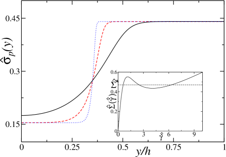
We numerically solve this integro-differential equation using a semi-implicit Crank-Nicolson algorithm numC . Once a solution is found, the selected stress Σ^superscript^Σ\widehat{\Sigma}^{\ast} is obtained using Eq. (2.8). Fig. 1 shows banding profiles σ^p(y^)subscript^𝜎𝑝^𝑦\hat{\sigma}_{p}(\hat{y}) for the function g(ξ)𝑔𝜉g(\xi) given by Eq. (2.3).

Refer to caption
Figure 1: The polymer stress σpsubscript𝜎𝑝\sigma_{p} as a function of the distance y^=y/h^𝑦𝑦\hat{y}=y/h from the lower plate for D^=0.0001^𝐷0.0001\hat{D}=0.0001 (dotted), D^=0.001^𝐷0.001\hat{D}=0.001 (dashed) and D^=0.01^𝐷0.01\hat{D}=0.01 (solid), for α=20𝛼20\alpha=20 and average shear rate γ~=2.60delimited-⟨⟩~𝛾2.60\langle\tilde{{\gamma}}\rangle=2.60. The selected stress is Σ^=0.470superscript^Σ0.470\widehat{\Sigma}^{\ast}=0.470 for D^=0.001^𝐷0.001\hat{D}=0.001 and D^=0.0001^𝐷0.0001\hat{D}=0.0001; and Σ^=0.471superscript^Σ0.471\widehat{\Sigma}^{\ast}=0.471 for D^=0.01^𝐷0.01\hat{D}=0.01. The inset shows the corresponding constitutive curve, shear stress Σ^^Σ\widehat{\Sigma} as a function of γ˙^^˙𝛾\hat{\dot{\gamma}}, for α=20𝛼20\alpha=20.
Refer to caption
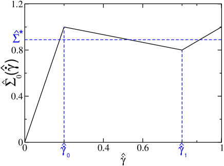
Figure 2: The selected stress Σ^superscript^Σ\widehat{\Sigma}^{\ast} and the piecewise linear function Σ^0(γ˙^)subscript^Σ0^˙𝛾\widehat{\Sigma}_{0}(\hat{\dot{\gamma}}) as a function of γ˙^^˙𝛾\hat{\dot{\gamma}} for γ˙^0=0.2subscript^˙𝛾00.2\hat{\dot{\gamma}}_{0}=0.2, γ˙^1=0.8subscript^˙𝛾10.8\hat{\dot{\gamma}}_{1}=0.8, Ac=5subscript𝐴𝑐5A_{c}=5; the selected stress is Σ^=0.891superscript^Σ0.891\widehat{\Sigma}^{\ast}=0.891.
Refer to caption
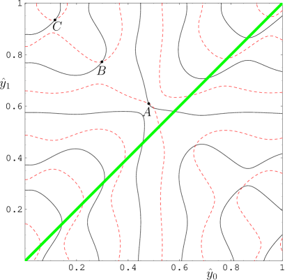
Figure 3: The solutions A𝐴A, B𝐵B, C𝐶C, for y^0subscript^𝑦0\hat{y}_{0} and y^1subscript^𝑦1\hat{y}_{1}, for the parameter values: Ac=5,α=1,γ˙^=0.50,γ˙^0=0.2,γ˙^1=0.8formulae-sequencesubscript𝐴𝑐5formulae-sequence𝛼1formulae-sequencedelimited-⟨⟩^˙𝛾0.50formulae-sequencesubscript^˙𝛾00.2subscript^˙𝛾10.8A_{c}=5,\alpha=1,\langle{\hat{\dot{\gamma}}}\rangle=0.50,\hat{\dot{\gamma}}_{0}=0.2,\hat{\dot{\gamma}}_{1}=0.8, and D^=0.001^𝐷0.001\hat{D}=0.001. The dashed curves correspond to Eq. (2.17) and the solid ones to Eq. (2.18). The physical range of solutions is in the upper left triangle, 0<y0<y1<10subscript𝑦0subscript𝑦110<y_{0}<y_{1}<1.
Refer to caption
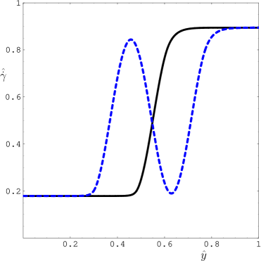
Figure 4: Two stationary solutions corresponding to A𝐴A (solid curve) and B𝐵B (dashed curve). An additional third solution with one more oscillation is not shown.

To better understand stress selection we will generalize g(ξ)𝑔𝜉g(\xi) to a function that allows explicit analytic calculations, but is sufficiently general to describe shear banding. The calculations discussed in the main text concern this general model. However, for comparison we also reproduce the calculations for the function g𝑔g defined in Eq. (2.3), in Appendix C. The most essential characteristic of g𝑔g is that it vanishes for small and large shear rates, so that the function Σ^(x)=x/α+g(x)^Σ𝑥𝑥𝛼𝑔𝑥\widehat{\Sigma}(x)=x/\alpha+g(x) is nonmonotonic with a maximum and a minimum. A simple piecewise linear function showing this behavior is

Σ^0(γ˙^)={Acγ˙^α(γ˙^<γ˙^0)[Acγ˙^0γ˙^1γ˙^0γ˙^1](γ˙^γ˙^0)α+Acγ˙^0α(γ˙^0<γ˙^<γ˙^1)γ˙^α(γ˙^>γ˙^1),subscript^Σ0^˙𝛾casessubscript𝐴𝑐^˙𝛾𝛼^˙𝛾subscript^˙𝛾0delimited-[]subscript𝐴𝑐subscript^˙𝛾0subscript^˙𝛾1subscript^˙𝛾0subscript^˙𝛾1^˙𝛾subscript^˙𝛾0𝛼subscript𝐴𝑐subscript^˙𝛾0𝛼subscript^˙𝛾0^˙𝛾subscript^˙𝛾1^˙𝛾𝛼^˙𝛾subscript^˙𝛾1\displaystyle\widehat{\Sigma}_{0}(\hat{\dot{\gamma}})=\begin{cases}\displaystyle\frac{A_{c}\hat{\dot{\gamma}}}{\alpha}&(\hat{\dot{\gamma}}<\hat{\dot{\gamma}}_{0})\\[10.0pt] \displaystyle\left[\frac{A_{c}\hat{\dot{\gamma}}_{0}-\hat{\dot{\gamma}}_{1}}{\hat{\dot{\gamma}}_{0}-\hat{\dot{\gamma}}_{1}}\right]\frac{(\hat{\dot{\gamma}}-\hat{\dot{\gamma}}_{0})}{\alpha}+\frac{A_{c}\hat{\dot{\gamma}}_{0}}{\alpha}&(\hat{\dot{\gamma}}_{0}<\hat{\dot{\gamma}}<\hat{\dot{\gamma}}_{1})\\[10.0pt] \displaystyle\frac{\hat{\dot{\gamma}}}{\alpha}&(\hat{\dot{\gamma}}>\hat{\dot{\gamma}}_{1}),\end{cases} (2.12)

where Acγ˙^0>γ˙^1subscript𝐴𝑐subscript^˙𝛾0subscript^˙𝛾1A_{c}\hat{\dot{\gamma}}_{0}>\hat{\dot{\gamma}}_{1}. The form of Σ^0(γ˙^)subscript^Σ0^˙𝛾\widehat{\Sigma}_{0}(\hat{\dot{\gamma}}) is completely specified by the three parameters γ˙^0subscript^˙𝛾0\hat{\dot{\gamma}}_{0}, γ˙^1subscript^˙𝛾1\hat{\dot{\gamma}}_{1}, and Acsubscript𝐴𝑐A_{c}.

Using Σ^0(γ˙^)γ˙^/αsubscript^Σ0^˙𝛾^˙𝛾𝛼\widehat{\Sigma}_{0}(\hat{\dot{\gamma}})-\hat{\dot{\gamma}}/\alpha instead of g𝑔g in the equation of motion for σ^psubscript^𝜎𝑝\hat{\sigma}_{p}, and eliminating σ^psubscript^𝜎𝑝\hat{\sigma}_{p} using Eq. (2.1), the steady state condition for γ˙^^˙𝛾\hat{\dot{\gamma}} is given by

D^γ˙^′′+αΣ^=αΣ^0(γ˙^).^𝐷superscript^˙𝛾′′𝛼^Σ𝛼subscript^Σ0^˙𝛾\hat{D}\hat{\dot{\gamma}}^{\prime\prime}+\alpha\widehat{\Sigma}=\alpha\widehat{\Sigma}_{0}(\hat{\dot{\gamma}}). (2.13)

This is solved with Neumann boundary conditions for the stress at y^=0^𝑦0\hat{y}=0 and y^=1^𝑦1\hat{y}=1, leading to

γ˙^I(y^)subscript^˙𝛾𝐼^𝑦\displaystyle\hat{\dot{\gamma}}_{I}(\hat{y}) =c1cosh(AcD^y^)+αΣ^Acabsentsubscript𝑐1subscript𝐴𝑐^𝐷^𝑦𝛼^Σsubscript𝐴𝑐\displaystyle=c_{1}\cosh\left(\sqrt{\frac{A_{c}}{\hat{D}}}\hat{y}\right)+\alpha\frac{\widehat{\Sigma}}{A_{c}} (0<y^<y^0)0^𝑦subscript^𝑦0\displaystyle(0<\hat{y}<\hat{y}_{0}) (2.14a)
γ˙^II(y^)subscript^˙𝛾𝐼𝐼^𝑦\displaystyle\hat{\dot{\gamma}}_{II}(\hat{y}) =d1cos(zD^y^)+d2sin(zD^y^)+γ˙^0(Acγ˙^0αΣ^)Acγ˙^0γ˙^1(γ˙^0γ˙^1)absentsubscript𝑑1𝑧^𝐷^𝑦subscript𝑑2𝑧^𝐷^𝑦subscript^˙𝛾0subscript𝐴𝑐subscript^˙𝛾0𝛼^Σsubscript𝐴𝑐subscript^˙𝛾0subscript^˙𝛾1subscript^˙𝛾0subscript^˙𝛾1\displaystyle=d_{1}\cos\left(\sqrt{\frac{z}{\hat{D}}}{\hat{y}}\right)+d_{2}\sin\left(\sqrt{\frac{z}{\hat{D}}}{\hat{y}}\right)+\hat{\dot{\gamma}}_{0}-\frac{(A_{c}\hat{\dot{\gamma}}_{0}-\alpha\widehat{\Sigma})}{A_{c}\hat{\dot{\gamma}}_{0}-\hat{\dot{\gamma}}_{1}}(\hat{\dot{\gamma}}_{0}-\hat{\dot{\gamma}}_{1}) (y^0<y^<y^1)subscript^𝑦0^𝑦subscript^𝑦1\displaystyle(\hat{y}_{0}<\hat{y}<\hat{y}_{1}) (2.14b)
γ˙^III(y^)subscript^˙𝛾𝐼𝐼𝐼^𝑦\displaystyle\hat{\dot{\gamma}}_{III}(\hat{y}) =αΣ^+c2cosh(y^1D^)absent𝛼^Σsubscript𝑐2^𝑦1^𝐷\displaystyle=\alpha\widehat{\Sigma}+c_{2}\cosh\left(\frac{\hat{y}-1}{\sqrt{\hat{D}}}\right) (y^1<y^<1)subscript^𝑦1^𝑦1\displaystyle(\hat{y}_{1}<\hat{y}<1) (2.14c)

where z(Acγ˙^0γ˙^1)/(γ˙^1γ˙^0)𝑧subscript𝐴𝑐subscript^˙𝛾0subscript^˙𝛾1subscript^˙𝛾1subscript^˙𝛾0z\equiv(A_{c}\hat{\dot{\gamma}}_{0}-\hat{\dot{\gamma}}_{1})/(\hat{\dot{\gamma}}_{1}-\hat{\dot{\gamma}}_{0}), which can be recognized as the negative of the slope of the function Σ^0(γ˙^)subscript^Σ0^˙𝛾\widehat{\Sigma}_{0}(\hat{\dot{\gamma}}) between γ˙^0subscript^˙𝛾0\hat{\dot{\gamma}}_{0} and γ˙^1subscript^˙𝛾1\hat{\dot{\gamma}}_{1}. The profile obeys the following continuity conditions:

γ˙^I(y^0)subscript^˙𝛾𝐼subscript^𝑦0\displaystyle\hat{\dot{\gamma}}_{I}(\hat{y}_{0}) =γ˙^II(y^0)=γ˙^0absentsubscript^˙𝛾𝐼𝐼subscript^𝑦0subscript^˙𝛾0\displaystyle=\hat{\dot{\gamma}}_{II}(\hat{y}_{0})=\hat{\dot{\gamma}}_{0} (2.15)
γ˙^II(y^1)subscript^˙𝛾𝐼𝐼subscript^𝑦1\displaystyle\hat{\dot{\gamma}}_{II}(\hat{y}_{1}) =γ˙^III(y^1)=γ˙^1absentsubscript^˙𝛾𝐼𝐼𝐼subscript^𝑦1subscript^˙𝛾1\displaystyle=\hat{\dot{\gamma}}_{III}(\hat{y}_{1})=\hat{\dot{\gamma}}_{1} (2.16)
γ˙^I(y^0)superscriptsubscript^˙𝛾𝐼subscript^𝑦0\displaystyle\hat{\dot{\gamma}}_{I}^{\prime}(\hat{y}_{0}) =γ˙^II(y^0)absentsubscriptsuperscript^˙𝛾𝐼𝐼subscript^𝑦0\displaystyle=\hat{\dot{\gamma}}^{\prime}_{II}(\hat{y}_{0}) (2.17)
γ˙^II(y^1)superscriptsubscript^˙𝛾𝐼𝐼subscript^𝑦1\displaystyle\hat{\dot{\gamma}}_{II}^{\prime}(\hat{y}_{1}) =γ˙^III(y^1),absentsubscriptsuperscript^˙𝛾𝐼𝐼𝐼subscript^𝑦1\displaystyle=\hat{\dot{\gamma}}^{\prime}_{III}(\hat{y}_{1}), (2.18)

where again the prime denotes a y𝑦y-derivative, γ˙^=γ˙^/y^superscript^˙𝛾^˙𝛾^𝑦\hat{\dot{\gamma}}^{\prime}=\partial\hat{\dot{\gamma}}/\partial\hat{y}. These six conditions guarantee a smooth solution for the shear rate and stress and from them the four constants c1subscript𝑐1c_{1}, c2subscript𝑐2c_{2}, d1subscript𝑑1d_{1}, d2subscript𝑑2d_{2} and the locations y^0subscript^𝑦0\hat{y}_{0} and y^1subscript^𝑦1\hat{y}_{1} where the function Σ^0(γ˙^)subscript^Σ0^˙𝛾\widehat{\Sigma}_{0}(\hat{\dot{\gamma}}) switches from one piece to the next, can be determined. Appendix A contains expressions for the constants c1subscript𝑐1c_{1}, c2subscript𝑐2c_{2}, and d1subscript𝑑1d_{1}, d2subscript𝑑2d_{2} as functions of y^0subscript^𝑦0\hat{y}_{0} and y^1subscript^𝑦1\hat{y}_{1}. d1subscript𝑑1d_{1} and d2subscript𝑑2d_{2} are found by combining Eqs. (2.15) and (2.17). Eqs. (2.16) and (2.18) are then used to determine the values of y^0subscript^𝑦0\hat{y}_{0} and y^1subscript^𝑦1\hat{y}_{1}. The selected stress Σ^superscript^Σ\widehat{\Sigma}^{\ast} is determined by the constraint of an applied average shear rate γ˙^delimited-⟨⟩^˙𝛾\langle{\hat{\dot{\gamma}}}\rangle, which is given by Eq. (A.2). In a shear banding state the selected stress Σ^superscript^Σ\widehat{\Sigma}^{\ast} satisfies γ˙^1<Σ^<Acγ˙^0subscript^˙𝛾1superscript^Σsubscript𝐴𝑐subscript^˙𝛾0\hat{\dot{\gamma}}_{1}<\widehat{\Sigma}^{\ast}<A_{c}\hat{\dot{\gamma}}_{0}, and we must have γ˙^>0^˙𝛾0\hat{\dot{\gamma}}>0 on the interval y^[0,1]^𝑦01\hat{y}\in[0,1].

A graphical solution for y^0subscript^𝑦0\hat{y}_{0} and y^1subscript^𝑦1\hat{y}_{1}, for the case D^=0.001^𝐷0.001\hat{D}=0.001, Ac=5subscript𝐴𝑐5A_{c}=5 and γ˙^=0.5delimited-⟨⟩^˙𝛾0.5\langle\hat{\dot{\gamma}}\rangle=0.5, is depicted in Fig. 3, as the intersections of the contour plots of Eqs. (2.17) (dashed line) and (2.18) (solid line), which should simultaneously be obeyed by y^0subscript^𝑦0\hat{y}_{0} and y^1subscript^𝑦1\hat{y}_{1}. To solve these equations the expressions for the constants c1,c2,d1,d2subscript𝑐1subscript𝑐2subscript𝑑1subscript𝑑2c_{1},c_{2},d_{1},d_{2} from Appendix A are used, Eqs. (A.1), as well as expression (A.2) for the selected stress. The physical range of Fig. 3 is the upper left hand triangle 0<y^0<y^1<10subscript^𝑦0subscript^𝑦110<\hat{y}_{0}<\hat{y}_{1}<1, to the left of the diagonal line in Fig. 3.

Fig. 3 shows three intersection points corresponding to stationary solutions, denoted by A=(0.4806,0.6101)𝐴0.48060.6101A=(0.4806,0.6101), B=(0.2984,0.7726)𝐵0.29840.7726B=(0.2984,0.7726), and C=(0.1160,0.9345)𝐶0.11600.9345C=(0.1160,0.9345). The values of the selected stress Σ^superscript^Σ\widehat{\Sigma}^{\ast} associated with these solutions are 0.89440.89440.8944 for A𝐴A, 0.89460.89460.8946 for B𝐵B and 0.89490.89490.8949 for C𝐶C. The fourth intersection point (the companion of A𝐴A, with the unphysical value of Σ^=4.8superscript^Σ4.8\widehat{\Sigma}^{\ast}=4.8) is ignored, as it violates the condition γ˙^1<Σ^<Acγ˙^0subscript^˙𝛾1^Σsubscript𝐴𝑐subscript^˙𝛾0\hat{\dot{\gamma}}_{1}<\widehat{\Sigma}<A_{c}\hat{\dot{\gamma}}_{0}.

The first solution A𝐴A corresponds to the common shear rate profile depicted as a solid curve in Fig. 4. The stationary solution B𝐵B (shown dashed) has an extra oscillation in the interface region (Fig. 4), while the third solution C𝐶C has two oscillations (not shown). The selected stress changes monotonically as a function of an increasing number of oscillations in the resulting solution. The existence of multiple solutions for small diffusion constants is well-known in the context of pattern formation in reaction-diffusion models grindrod . Multiple solutions occur in our model when D^102less-than-or-similar-to^𝐷superscript102\hat{D}\lesssim 10^{-2}, with the multiplicity increasing for decreasing D^^𝐷\hat{D}. Having obtained the stationary solutions we next examine their stability by performing a linear perturbation analysis.

3 Linear stability analysis

3.1 Governing Equations and Matching Conditions

We study the linear stability of the piecewise linear model by introducing small perturbations to the stationary 1D solutions,

σ^p(x^,y^)subscript^𝜎𝑝^𝑥^𝑦\displaystyle\hat{\sigma}_{p}(\hat{x},\hat{y}) =σ^p1D(y^)+δσ^p(x^,y^)absentsuperscriptsubscript^𝜎𝑝1𝐷^𝑦𝛿subscript^𝜎𝑝^𝑥^𝑦\displaystyle=\hat{\sigma}_{p}^{1D}(\hat{y})+\delta\hat{\sigma}_{p}(\hat{x},\hat{y}) (3.1)
Σ^(x^)^Σ^𝑥\displaystyle\widehat{\Sigma}(\hat{x}) =Σ^1D+δΣ^(x^)absentsuperscript^Σ1𝐷𝛿^Σ^𝑥\displaystyle=\widehat{\Sigma}^{1D}+\delta\widehat{\Sigma}(\hat{x}) (3.2)
γ˙^(x^,y^)^˙𝛾^𝑥^𝑦\displaystyle\hat{\dot{\gamma}}(\hat{x},\hat{y}) =γ˙^1D(y^)+δγ˙^(x^,y^)absentsuperscript^˙𝛾1𝐷^𝑦𝛿^˙𝛾^𝑥^𝑦\displaystyle=\hat{\dot{\gamma}}^{1D}(\hat{y})+\delta\hat{\dot{\gamma}}(\hat{x},\hat{y}) (3.3)
𝒗^^𝒗\displaystyle\hat{\boldsymbol{v}} =(v^1D(y^)+δv^x^(x^,y^),δv^y^(x^,y^)),absentsuperscript^𝑣1𝐷^𝑦𝛿subscript^𝑣^𝑥^𝑥^𝑦𝛿subscript^𝑣^𝑦^𝑥^𝑦\displaystyle=(\hat{v}^{1D}(\hat{y})+\delta\hat{v}_{\hat{x}}(\hat{x},\hat{y}),\delta\hat{v}_{\hat{y}}(\hat{x},\hat{y})), (3.4)

where the superscript 1D denotes the stationary 1D solution. Perturbations in the shear rate, polymer stress and total stress are related by δΣ^=δσ^p+γ˙^/α𝛿^Σ𝛿subscript^𝜎𝑝^˙𝛾𝛼\delta\widehat{\Sigma}=\delta\hat{\sigma}_{p}+\hat{\dot{\gamma}}/\alpha, which can be recast as

δσ^p=δσ^p+δγ˙^/αdelimited-⟨⟩𝛿subscript^𝜎𝑝𝛿subscript^𝜎𝑝𝛿^˙𝛾𝛼\langle\delta\hat{\sigma}_{p}\rangle=\delta\hat{\sigma}_{p}+\delta\hat{\dot{\gamma}}/\alpha (3.5)

by averaging and using δγ˙^=0delimited-⟨⟩𝛿^˙𝛾0\langle\delta\hat{\dot{\gamma}}\rangle=0. Note that δγ˙^=0delimited-⟨⟩𝛿^˙𝛾0\langle\delta\hat{\dot{\gamma}}\rangle=0 implies that the average perturbation in the polymer stress δσ^pdelimited-⟨⟩𝛿subscript^𝜎𝑝\langle\delta\hat{\sigma}_{p}\rangle equals the perturbation in the total stress δΣ^𝛿^Σ\delta\widehat{\Sigma}, for γ˙^=α(δΣ^δσ^p)^˙𝛾𝛼𝛿^Σ𝛿subscript^𝜎𝑝\hat{\dot{\gamma}}=\alpha(\delta\widehat{\Sigma}-\delta\hat{\sigma}_{p}). The shear rate is given by γ˙^(x,y)=y^(v^1D(y^)+δv^x(x^,y^))^˙𝛾𝑥𝑦subscript^𝑦superscript^𝑣1𝐷^𝑦𝛿subscript^𝑣𝑥^𝑥^𝑦\hat{\dot{\gamma}}(x,y)=\partial_{{\hat{y}}}(\hat{v}^{1D}(\hat{y})+\delta\hat{v}_{x}(\hat{x},\hat{y})), so that δγ˙^(x^,y^)=y^δvx^(x^,y^)𝛿^˙𝛾^𝑥^𝑦subscript^𝑦𝛿subscript𝑣^𝑥^𝑥^𝑦\delta\hat{\dot{\gamma}}(\hat{x},\hat{y})=\partial_{\hat{y}}\delta v_{\hat{x}}(\hat{x},\hat{y}). Because the flow is incompressible, a variation of the velocity in the x𝑥x-direction must be accompanied by a compensating variation of the velocity in the y𝑦y-direction, which obeys

y^δv^y(x^,y^)=x^δv^x(x^,y^).subscript^𝑦𝛿subscript^𝑣𝑦^𝑥^𝑦subscript^𝑥𝛿subscript^𝑣𝑥^𝑥^𝑦\partial_{\hat{y}}\delta\hat{v}_{y}(\hat{x},\hat{y})=-\partial_{\hat{x}}\delta\hat{v}_{x}(\hat{x},\hat{y}). (3.6)

We recall that the equation of motion of the polymer stress is given by

(t^+𝐯^)σ^p=Σ^0(γ˙^)Σ^+D^2σ^p.subscript^𝑡^𝐯subscript^𝜎𝑝subscript^Σ0^˙𝛾^Σ^𝐷superscript2subscript^𝜎𝑝(\partial_{\hat{t}}+\hat{\bf{v}}\cdot\nabla)\hat{\sigma}_{p}=\widehat{\Sigma}_{0}(\hat{\dot{\gamma}})-\widehat{\Sigma}+\hat{D}\nabla^{2}\hat{\sigma}_{p}. (3.7)

This equation can be recast in a differential equation for the shear rate γ˙^^˙𝛾\hat{\dot{\gamma}}, by using δσ^p=δΣ^δγ˙^/α𝛿subscript^𝜎𝑝𝛿^Σ𝛿^˙𝛾𝛼\delta\hat{\sigma}_{p}=\delta\widehat{\Sigma}-\delta\hat{\dot{\gamma}}/\alpha, from which we find to first order in all perturbations

t^δγ˙^+v^1D(y^)x^δγ˙^+δv^y^y^γ˙^1D(y^)=(t^+v^x^1Dx^)αδΣ^+D^[x^x^+y^y^]δγ˙^D^x^x^αδΣ^αΣ^0(γ˙^1D+δγ˙^)+αΣ^0(γ˙^1D),subscript^𝑡𝛿^˙𝛾superscript^𝑣1𝐷^𝑦subscript^𝑥𝛿^˙𝛾𝛿subscript^𝑣^𝑦subscript^𝑦superscript^˙𝛾1𝐷^𝑦subscript^𝑡superscriptsubscript^𝑣^𝑥1𝐷subscript^𝑥𝛼𝛿^Σ^𝐷delimited-[]subscript^𝑥^𝑥subscript^𝑦^𝑦𝛿^˙𝛾^𝐷subscript^𝑥^𝑥𝛼𝛿^Σ𝛼subscript^Σ0superscript^˙𝛾1𝐷𝛿^˙𝛾𝛼subscript^Σ0superscript^˙𝛾1𝐷\partial_{\hat{t}}\delta\hat{\dot{\gamma}}+\hat{v}^{1D}(\hat{y})\partial_{{\hat{x}}}\delta\hat{\dot{\gamma}}+\delta\hat{v}_{\hat{y}}\partial_{{\hat{y}}}\hat{\dot{\gamma}}^{1D}(\hat{y})=(\partial_{\hat{t}}+\hat{v}_{\hat{x}}^{1D}\partial_{\hat{x}})\alpha\delta\widehat{\Sigma}\\ +\hat{D}\left[\partial_{\hat{x}\hat{x}}+\partial_{\hat{y}\hat{y}}\right]\delta\hat{\dot{\gamma}}-\hat{D}\partial_{\hat{x}\hat{x}}\alpha\delta\widehat{\Sigma}-\alpha\widehat{\Sigma}_{0}(\hat{\dot{\gamma}}^{1D}+\delta\hat{\dot{\gamma}})+\alpha\widehat{\Sigma}_{0}(\hat{\dot{\gamma}}^{1D}), (3.8)

where we explicitly kept Σ^0(γ˙^1D+δγ˙^)subscript^Σ0superscript^˙𝛾1𝐷𝛿^˙𝛾\widehat{\Sigma}_{0}(\hat{\dot{\gamma}}^{1D}+\delta\hat{\dot{\gamma}}) and Σ^0(γ˙^1D)subscript^Σ0superscript^˙𝛾1𝐷\widehat{\Sigma}_{0}(\hat{\dot{\gamma}}^{1D}) in order to avoid differentiating the function Σ^0subscript^Σ0\widehat{\Sigma}_{0} with respect to γ˙^^˙𝛾\hat{\dot{\gamma}}. This was done as the function Σ^0subscript^Σ0\widehat{\Sigma}_{0} is continuous for all γ˙^^˙𝛾\hat{\dot{\gamma}}, but non-differentiable in the turning points of the stress at γ˙^0,γ˙^1subscript^˙𝛾0subscript^˙𝛾1\hat{\dot{\gamma}}_{0},\hat{\dot{\gamma}}_{1}.

Using Eqs. (3.5) and (3.6) we can easily express the perturbed velocities δv^x(x^,y^)𝛿subscript^𝑣𝑥^𝑥^𝑦\delta\hat{v}_{x}(\hat{x},\hat{y}) and δv^y(x^,y^)𝛿subscript^𝑣𝑦^𝑥^𝑦\delta\hat{v}_{y}(\hat{x},\hat{y}) in terms of δγ˙^𝛿^˙𝛾\delta\hat{\dot{\gamma}}. Starting from the identity δvx^(x^,y^,t^)y^=δγ˙^𝛿subscript𝑣^𝑥^𝑥^𝑦^𝑡^𝑦𝛿^˙𝛾\frac{\partial\delta v_{\hat{x}}(\hat{x},\hat{y},\hat{t})}{\partial\hat{y}}=\delta\hat{\dot{\gamma}}, we integrate from 00 to y^^𝑦\hat{y} and use the no slip boundary condition at y^=0^𝑦0\hat{y}=0, which yields

δv^x(x^,y^)=0y^δγ˙^(x^,y)𝑑y.𝛿subscript^𝑣𝑥^𝑥^𝑦superscriptsubscript0^𝑦𝛿^˙𝛾^𝑥superscript𝑦differential-dsuperscript𝑦\displaystyle\delta\hat{v}_{x}(\hat{x},\hat{y})=\int_{0}^{\hat{y}}\delta\hat{\dot{\gamma}}(\hat{x},y^{\prime})dy^{\prime}. (3.9)

If one next differentiates δv^x(x^,y^)𝛿subscript^𝑣𝑥^𝑥^𝑦\delta\hat{v}_{x}(\hat{x},\hat{y}) with respect to x^^𝑥\hat{x} and substitutes the resulting expression in Eq. (3.6), only one integration with respect to y^^𝑦\hat{y} (again starting from 00 and using no slip boundary conditions) is necessary to obtain the perturbed velocity in the y^^𝑦\hat{y} direction

δv^y(x^,y^)=𝛿subscript^𝑣𝑦^𝑥^𝑦absent\displaystyle\delta\hat{v}_{y}(\hat{x},\hat{y})= 0y^[0yx^δγ˙^(x^,y′′)dy′′]𝑑y.superscriptsubscript0^𝑦delimited-[]superscriptsubscript0superscript𝑦subscript^𝑥𝛿^˙𝛾^𝑥superscript𝑦′′𝑑superscript𝑦′′differential-dsuperscript𝑦\displaystyle-\int_{0}^{\hat{y}}\left[\int_{0}^{y^{\prime}}\partial_{\hat{x}}\delta\hat{\dot{\gamma}}(\hat{x},y^{\prime\prime})dy^{\prime\prime}\right]\,dy^{\prime}. (3.10)

Hence the equation for the shear rate perturbation δγ˙^𝛿^˙𝛾\delta\hat{\dot{\gamma}} (3.8) can be expressed entirely in terms of δγ˙^𝛿^˙𝛾\delta\hat{\dot{\gamma}}, integrals over δγ˙^𝛿^˙𝛾\delta\hat{\dot{\gamma}} and δΣ^𝛿^Σ\delta\widehat{\Sigma}. Perturbations in the shear rate must be continuous across the matching points of the bands, which are yet to be found. These follow from demanding

(γ˙^1D+δγ˙^)|y^0+δy^0=γ˙^0,(γ˙^1D+δγ˙^)|y^1+δy^1=γ˙^1,formulae-sequenceevaluated-atsuperscript^˙𝛾1𝐷𝛿^˙𝛾subscript^𝑦0𝛿subscript^𝑦0subscript^˙𝛾0evaluated-atsuperscript^˙𝛾1𝐷𝛿^˙𝛾subscript^𝑦1𝛿subscript^𝑦1subscript^˙𝛾1\displaystyle\left.\left(\widehat{\dot{\gamma}}^{1D}+\delta\widehat{\dot{\gamma}}\right)\right|_{\hat{y}_{0}+\delta{\hat{y}_{0}}}=\widehat{\dot{\gamma}}_{0},\,\,\,\,\,\,\,\left.\left(\widehat{\dot{\gamma}}^{1D}+\delta\widehat{\dot{\gamma}}\right)\right|_{\hat{y}_{1}+\delta{\hat{y}_{1}}}=\widehat{\dot{\gamma}}_{1}, (3.11)

that is, the matching points are shifted by perturbations δy^𝛿^𝑦\delta\hat{y} needed to bring the local shear rate to the matching points in the constitutive relation Σ0(γ˙^)subscriptΣ0^˙𝛾\Sigma_{0}(\hat{\dot{\gamma}}). Hence we split the interval [0,1]01[0,1] into three parts: (I)𝐼(I), y[0,y~0]𝑦0subscript~𝑦0y\in[0,\tilde{y}_{0}]; (II)𝐼𝐼(II), y[y~0,y~1]𝑦subscript~𝑦0subscript~𝑦1y\in[\tilde{y}_{0},\tilde{y}_{1}], and (III)𝐼𝐼𝐼(III), y[y~1,1]𝑦subscript~𝑦11y\in[\tilde{y}_{1},1], where y~i=y^i+δy^i(x^,t^),i=1,2formulae-sequencesubscript~𝑦𝑖subscript^𝑦𝑖𝛿subscript^𝑦𝑖^𝑥^𝑡𝑖12\tilde{y}_{i}=\hat{y}_{i}+\delta\hat{y}_{i}(\hat{x},\hat{t}),i=1,2. The equations of motion for the perturbations in the polymer stress are, from Eq. (3.8)

t^δγ˙^Isubscript^𝑡𝛿superscript^˙𝛾𝐼\displaystyle\partial_{\hat{t}}\delta\hat{\dot{\gamma}}^{I} =D^2δγ˙^Iv^x^1D(y^)x^δγ˙^Iδv^y^(x^,y^)y^γ˙^1DAcδγ˙^I+F(αδΣ^,t^)absent^𝐷superscript2𝛿superscript^˙𝛾𝐼superscriptsubscript^𝑣^𝑥1𝐷^𝑦subscript^𝑥𝛿superscript^˙𝛾𝐼𝛿subscript^𝑣^𝑦^𝑥^𝑦subscript^𝑦superscript^˙𝛾1𝐷subscript𝐴𝑐𝛿superscript^˙𝛾𝐼𝐹𝛼𝛿^Σ^𝑡\displaystyle=\hat{D}\nabla^{2}\delta\hat{\dot{\gamma}}^{I}-\hat{v}_{\hat{x}}^{1D}(\hat{y})\partial_{\hat{x}}\delta\hat{\dot{\gamma}}^{I}-\delta\hat{v}_{\hat{y}}(\hat{x},\hat{y})\partial_{\hat{y}}\hat{\dot{\gamma}}^{1D}-A_{c}\delta\hat{\dot{\gamma}}^{I}+F(\alpha\delta\widehat{\Sigma},\hat{t}) (3.12a)
t^δγ˙^IIsubscript^𝑡𝛿superscript^˙𝛾𝐼𝐼\displaystyle\partial_{\hat{t}}\delta\hat{\dot{\gamma}}^{II} =D^2δγ˙^IIv^x^1D(y^)x^δγ˙^IIδv^y^(x^,y^)y^γ˙^1D+zδγ˙^II+F(αδΣ^,t^)absent^𝐷superscript2𝛿superscript^˙𝛾𝐼𝐼superscriptsubscript^𝑣^𝑥1𝐷^𝑦subscript^𝑥𝛿superscript^˙𝛾𝐼𝐼𝛿subscript^𝑣^𝑦^𝑥^𝑦subscript^𝑦superscript^˙𝛾1𝐷𝑧𝛿superscript^˙𝛾𝐼𝐼𝐹𝛼𝛿^Σ^𝑡\displaystyle=\hat{D}\nabla^{2}\delta\hat{\dot{\gamma}}^{II}-\hat{v}_{\hat{x}}^{1D}(\hat{y})\partial_{\hat{x}}\delta\hat{\dot{\gamma}}^{II}-\delta\hat{v}_{\hat{y}}(\hat{x},\hat{y})\partial_{\hat{y}}\hat{\dot{\gamma}}^{1D}+z\delta\hat{\dot{\gamma}}^{II}+F(\alpha\delta\widehat{\Sigma},\hat{t}) (3.12b)
t^δγ˙^IIIsubscript^𝑡𝛿superscript^˙𝛾𝐼𝐼𝐼\displaystyle\partial_{\hat{t}}\delta\hat{\dot{\gamma}}^{III} =D^2δγ˙^IIIv^x^1D(y^)x^δγ˙^IIIδv^y^(x^,y^)y^γ˙^1Dδγ˙^III+F(αδΣ^,t^)absent^𝐷superscript2𝛿superscript^˙𝛾𝐼𝐼𝐼superscriptsubscript^𝑣^𝑥1𝐷^𝑦subscript^𝑥𝛿superscript^˙𝛾𝐼𝐼𝐼𝛿subscript^𝑣^𝑦^𝑥^𝑦subscript^𝑦superscript^˙𝛾1𝐷𝛿superscript^˙𝛾𝐼𝐼𝐼𝐹𝛼𝛿^Σ^𝑡\displaystyle=\hat{D}\nabla^{2}\delta\hat{\dot{\gamma}}^{III}-\hat{v}_{\hat{x}}^{1D}(\hat{y})\partial_{\hat{x}}\delta\hat{\dot{\gamma}}^{III}-\delta\hat{v}_{\hat{y}}(\hat{x},\hat{y})\partial_{\hat{y}}\hat{\dot{\gamma}}^{1D}-\delta\hat{\dot{\gamma}}^{III}+F(\alpha\delta\widehat{\Sigma},\hat{t}) (3.12c)

where we defined F(αδΣ^,t^)=(t^+v^x^1Dx^D^x^x^)αδΣ^(x^,t^)𝐹𝛼𝛿^Σ^𝑡subscript^𝑡superscriptsubscript^𝑣^𝑥1𝐷subscript^𝑥^𝐷subscript^𝑥^𝑥𝛼𝛿^Σ^𝑥^𝑡F(\alpha\delta\widehat{\Sigma},\hat{t})=(\partial_{\hat{t}}+\hat{v}_{\hat{x}}^{1D}\partial_{\hat{x}}-\hat{D}\partial_{\hat{x}\hat{x}})\alpha\delta\widehat{\Sigma}(\hat{x},\hat{t}). Eqs. (3.12) must be supplemented with boundary conditions the matching points. At y^=y~0^𝑦subscript~𝑦0\hat{y}=\tilde{y}_{0} this condition can be found from Eq. (3.11),

γ˙^1D(y^0+δy^0(x^,t^))+δγ˙^(y^0+δy^0(x^,t^))=γ˙^0,superscript^˙𝛾1𝐷subscript^𝑦0𝛿subscript^𝑦0^𝑥^𝑡𝛿^˙𝛾subscript^𝑦0𝛿subscript^𝑦0^𝑥^𝑡subscript^˙𝛾0\displaystyle\hat{\dot{\gamma}}^{1D}(\hat{y}_{0}+\delta\hat{y}_{0}(\hat{x},\hat{t}))+\delta\hat{\dot{\gamma}}(\hat{y}_{0}+\delta\hat{y}_{0}(\hat{x},\hat{t}))=\hat{\dot{\gamma}}_{0}, (3.13)

which leads, to first order in the perturbed quantities, to

δγ˙^(y^0,x^,t^)=(γ˙^1Dy^)y^0δy^0(x^,t^).𝛿^˙𝛾subscript^𝑦0^𝑥^𝑡subscriptsuperscript^˙𝛾1𝐷^𝑦subscript^𝑦0𝛿subscript^𝑦0^𝑥^𝑡\displaystyle\delta\hat{\dot{\gamma}}(\hat{y}_{0},\hat{x},\hat{t})=-\left(\frac{\partial\hat{\dot{\gamma}}^{1D}}{\partial\hat{y}}\right)_{\hat{y}_{0}}\delta\hat{y}_{0}(\hat{x},\hat{t}). (3.14)

Eq. (3.14) relates the change in the shear rate to a shift in the interface position. The boundary condition at y^=y~1^𝑦subscript~𝑦1\hat{y}=\tilde{y}_{1} is derived similarly. From Eq. (3.14) we immediately retrieve the shift in the value of y0subscript𝑦0y_{0}, and hence the new position of the two shear bands, once δγ˙^𝛿^˙𝛾\delta\hat{\dot{\gamma}} is known. To deal with the inhomogeneous (time dependent) boundary conditions in region (II)𝐼𝐼(II) we define a new function q(x^,y^,t^)𝑞^𝑥^𝑦^𝑡q(\hat{x},\hat{y},\hat{t}) by

q(x^,y^,t^)𝑞^𝑥^𝑦^𝑡\displaystyle q(\hat{x},\hat{y},\hat{t}) =δγ˙^II(x^,y^,t^)+(y^y^1)δγ˙^(y^0,x^,t^)y^1y^0(y^y^0)δγ˙^(y^1,x^,t^)y^1y^0δγ˙^II(x^,y^,t^)+G(x^,y^,t^),absent𝛿superscript^˙𝛾𝐼𝐼^𝑥^𝑦^𝑡^𝑦subscript^𝑦1𝛿^˙𝛾subscript^𝑦0^𝑥^𝑡subscript^𝑦1subscript^𝑦0^𝑦subscript^𝑦0𝛿^˙𝛾subscript^𝑦1^𝑥^𝑡subscript^𝑦1subscript^𝑦0𝛿superscript^˙𝛾𝐼𝐼^𝑥^𝑦^𝑡𝐺^𝑥^𝑦^𝑡\displaystyle=\delta\hat{\dot{\gamma}}^{II}(\hat{x},\hat{y},\hat{t})+\frac{(\hat{y}-\hat{y}_{1})\delta\hat{\dot{\gamma}}(\hat{y}_{0},\hat{x},\hat{t})}{\hat{y}_{1}-\hat{y}_{0}}-\frac{(\hat{y}-\hat{y}_{0})\delta\hat{\dot{\gamma}}(\hat{y}_{1},\hat{x},\hat{t})}{\hat{y}_{1}-\hat{y}_{0}}\,{\equiv}\,\delta\hat{\dot{\gamma}}^{II}(\hat{x},\hat{y},\hat{t})+G(\hat{x},\hat{y},\hat{t}), (3.15)

which satisfies continuity at the matching points. Hence, the function q(x^,y^,t^)𝑞^𝑥^𝑦^𝑡q(\hat{x},\hat{y},\hat{t}) vanishes at the boundary points by construction. In Eq. (3.15) we introduced the function G(x^,y^,t^)𝐺^𝑥^𝑦^𝑡G(\hat{x},\hat{y},\hat{t}) for notational convenience. Using Eq. (3.12b), we find the following differential equation for q𝑞q:

t^q=zq+D^2qzG+F(αδΣ^,t^)+F(G,t^)v^x^1D(y^)x^qδv^y^(x^,y^)y^γ˙^1D.subscript^𝑡𝑞𝑧𝑞^𝐷superscript2𝑞𝑧𝐺𝐹𝛼𝛿^Σ^𝑡𝐹𝐺^𝑡superscriptsubscript^𝑣^𝑥1𝐷^𝑦subscript^𝑥𝑞𝛿subscript^𝑣^𝑦^𝑥^𝑦subscript^𝑦superscript^˙𝛾1𝐷\displaystyle\partial_{\hat{t}}q=zq+\hat{D}\nabla^{2}q-zG+F(\alpha\delta\widehat{\Sigma},\hat{t})+F(G,\hat{t})-\hat{v}_{\hat{x}}^{1D}(\hat{y})\partial_{\hat{x}}q-\delta\hat{v}_{\hat{y}}(\hat{x},\hat{y})\partial_{\hat{y}}\hat{\dot{\gamma}}^{1D}. (3.16)

Now that we have derived the governing equations for the perturbations, we study their stability properties by employing a Fourier expansion in spatial coordinates.

3.2 Fourier Expansion

We next expand the shear rate perturbation δγ˙^𝛿^˙𝛾\delta\hat{\dot{\gamma}} in Fourier modes, within the three regions, consistent with the boundary conditions γ˙^=0superscript^˙𝛾0\hat{\dot{\gamma}}^{\prime}=0 at y^=0^𝑦0\hat{y}=0 and y^=1^𝑦1\hat{y}=1. This results in a continuous but non-smooth function δγ˙^𝛿^˙𝛾\delta\hat{\dot{\gamma}} over the entire interval [0,1]01[0,1]:

δγ˙^I(x^,y^,t^)𝛿superscript^˙𝛾𝐼^𝑥^𝑦^𝑡\displaystyle\delta\hat{\dot{\gamma}}^{I}(\hat{x},\hat{y},\hat{t}) =n=0cos(πy^(2n+1)2y~0)An(x^,t^)+δγ˙^(y^0,x^,t^)absentsuperscriptsubscript𝑛0𝜋^𝑦2𝑛12subscript~𝑦0subscript𝐴𝑛^𝑥^𝑡𝛿^˙𝛾subscript^𝑦0^𝑥^𝑡\displaystyle=\sum_{n=0}^{\infty}\cos\left(\frac{\pi\hat{y}(2n+1)}{2\tilde{y}_{0}}\right)A_{n}(\hat{x},\hat{t})+\delta\hat{\dot{\gamma}}(\hat{y}_{0},\hat{x},\hat{t}) (0<y^<y~0)0^𝑦subscript~𝑦0\displaystyle(0<\hat{y}<\tilde{y}_{0}) (3.17a)
q(x^,y^,t^)𝑞^𝑥^𝑦^𝑡\displaystyle q(\hat{x},\hat{y},\hat{t}) =n=1Bn(x^,t^)sin(πn(y^y^0)y^1y^0)absentsuperscriptsubscript𝑛1subscript𝐵𝑛^𝑥^𝑡𝜋𝑛^𝑦subscript^𝑦0subscript^𝑦1subscript^𝑦0\displaystyle=\sum_{n=1}^{\infty}B_{n}(\hat{x},\hat{t})\sin\left(\frac{\pi n(\hat{y}-\hat{y}_{0})}{\hat{y}_{1}-\hat{y}_{0}}\right) (y~0<y^<y~1)subscript~𝑦0^𝑦subscript~𝑦1\displaystyle(\tilde{y}_{0}<\hat{y}<\tilde{y}_{1}) (3.17b)
δγ˙^III(x^,y^,t^)𝛿superscript^˙𝛾𝐼𝐼𝐼^𝑥^𝑦^𝑡\displaystyle\delta\hat{\dot{\gamma}}^{III}(\hat{x},\hat{y},\hat{t}) =n=0cos(π(y^1)(2n+1)2(1y~1))Dn(x^,t^)+δγ˙^(y^1,x^,t^)absentsuperscriptsubscript𝑛0𝜋^𝑦12𝑛121subscript~𝑦1subscript𝐷𝑛^𝑥^𝑡𝛿^˙𝛾subscript^𝑦1^𝑥^𝑡\displaystyle=\sum_{n=0}^{\infty}\cos\left(\frac{\pi(\hat{y}-1)(2n+1)}{2(1-\tilde{y}_{1})}\right)D_{n}(\hat{x},\hat{t})+\delta\hat{\dot{\gamma}}(\hat{y}_{1},\hat{x},\hat{t}) (y~1<y^<1).subscript~𝑦1^𝑦1\displaystyle(\tilde{y}_{1}<\hat{y}<1). (3.17c)

Only odd cosine modes contribute in regions I𝐼I and III𝐼𝐼𝐼III because we require zero derivatives at the ends of the interval [0,1]01[0,1] and a matching condition at the right, respectively left, ends of the intervals [0,y~0]0subscript~𝑦0[0,\tilde{y}_{0}] and [y~1,1]subscript~𝑦11[\tilde{y}_{1},1]. If one substitutes y^=y^0^𝑦subscript^𝑦0\hat{y}=\hat{y}_{0} in Eq. (3.17a) one finds δγ˙^I=δγ˙^(y^0,x^,t^)𝛿superscript^˙𝛾𝐼𝛿^˙𝛾subscript^𝑦0^𝑥^𝑡\delta\hat{\dot{\gamma}}^{I}=\delta\hat{\dot{\gamma}}(\hat{y}_{0},\hat{x},\hat{t}), which coincides with the boundary value of δγ˙^𝛿^˙𝛾\delta\hat{\dot{\gamma}} in y^0subscript^𝑦0\hat{y}_{0}, derived above in Eq. (3.11), which guarantees continuity of δγ˙^(x^,y^,t^)𝛿^˙𝛾^𝑥^𝑦^𝑡\delta\hat{\dot{\gamma}}(\hat{x},\hat{y},\hat{t}) throughout the interval [0,1]01[0,1]

One can easily demonstrate that the solution of Eqs. (3.17) is non-smooth, by trying to match the derivatives at y^=y^0,y^1^𝑦subscript^𝑦0subscript^𝑦1\hat{y}=\hat{y}_{0},\,\hat{y}_{1} using Eqs. (3.17). We will not reproduce these calculation here, but only note that the narrower the interface, that is the smaller y^1y^0subscript^𝑦1subscript^𝑦0\hat{y}_{1}-\hat{y}_{0}, the closer the matching at the the interface points y^0subscript^𝑦0\hat{y}_{0} and y^1subscript^𝑦1\hat{y}_{1}. The piecewise linear model will in this limit approach the smooth model defined by Eq. (2.3).

We therefore conclude that the perturbations are in general only continuous. To obtain an equation linking δγ˙^(y^0,x^,t^)𝛿^˙𝛾subscript^𝑦0^𝑥^𝑡\delta\hat{\dot{\gamma}}(\hat{y}_{0},\hat{x},\hat{t}) and δγ˙^(y^1,x^,t^)𝛿^˙𝛾subscript^𝑦1^𝑥^𝑡\delta\hat{\dot{\gamma}}(\hat{y}_{1},\hat{x},\hat{t}) we invoke the constraint δ^γ˙=0delimited-⟨⟩^𝛿˙𝛾0\langle\hat{\delta}{\dot{\gamma}}\rangle=0, from which we find

δγ˙^(y^0,x^,t^)2(y^0+y^1)+δγ˙^(y^1,x^,t^)2(2y^1y^0)=n=0An(1)n2y0(2n+1)πn=02(1y^1)Dn(1)n(2n+1)π(y1^y^0)n=1Bn(1(1)n)nπ.𝛿^˙𝛾subscript^𝑦0^𝑥^𝑡2subscript^𝑦0subscript^𝑦1𝛿^˙𝛾subscript^𝑦1^𝑥^𝑡22subscript^𝑦1subscript^𝑦0superscriptsubscript𝑛0subscript𝐴𝑛superscript1𝑛2subscript𝑦02𝑛1𝜋superscriptsubscript𝑛021subscript^𝑦1subscript𝐷𝑛superscript1𝑛2𝑛1𝜋^subscript𝑦1subscript^𝑦0superscriptsubscript𝑛1subscript𝐵𝑛1superscript1𝑛𝑛𝜋\displaystyle\frac{\delta\hat{\dot{\gamma}}(\hat{y}_{0},\hat{x},\hat{t})}{2}\left(\hat{y}_{0}+\hat{y}_{1}\right)+\frac{\delta\hat{\dot{\gamma}}(\hat{y}_{1},\hat{x},\hat{t})}{2}\left(2-\hat{y}_{1}-\hat{y}_{0}\right)=-\sum_{n=0}^{\infty}\frac{A_{n}(-1)^{n}2y_{0}}{(2n+1)\pi}-\sum_{n=0}^{\infty}\frac{2(1-\hat{y}_{1})D_{n}(-1)^{n}}{(2n+1)\pi}-\!(\hat{y_{1}}-\hat{y}_{0})\sum_{n=1}^{\infty}\frac{B_{n}(1-(-1)^{n})}{n\pi}. (3.18)

Eq. (3.18) constitutes the final equation needed to close the system, in a way which is similar to the method we used in section 2 to deduce the value of Σ^^Σ\widehat{\Sigma}, as we will now demonstrate.

The general idea is to find the governing equation for the amplitudes Ansubscript𝐴𝑛A_{n}, Bnsubscript𝐵𝑛B_{n}, Dnsubscript𝐷𝑛D_{n} from Eqs. (3.12) by projecting out the cosine (for Ansubscript𝐴𝑛A_{n} and Dnsubscript𝐷𝑛D_{n}) and sine modes (for Bnsubscript𝐵𝑛B_{n}). The evolution for δγ˙^(y^1,x^,t^)𝛿^˙𝛾subscript^𝑦1^𝑥^𝑡\delta\hat{\dot{\gamma}}(\hat{y}_{1},\hat{x},\hat{t}) and δγ˙^(y^0,x^,t^)𝛿^˙𝛾subscript^𝑦0^𝑥^𝑡\delta\hat{\dot{\gamma}}(\hat{y}_{0},\hat{x},\hat{t}) can be obtained by integrating Eqs. (3.12a) and (3.12c) over their respective intervals. This is most easily done in the Fourier domain, so we expand An(x^,t^)subscript𝐴𝑛^𝑥^𝑡A_{n}(\hat{x},\hat{t}), Bn(x^,t^)subscript𝐵𝑛^𝑥^𝑡B_{n}(\hat{x},\hat{t}), Dn(x^,t^)subscript𝐷𝑛^𝑥^𝑡D_{n}(\hat{x},\hat{t}), δΣ^(x^,t^)𝛿^Σ^𝑥^𝑡\delta\widehat{\Sigma}(\hat{x},\hat{t}), and δγ˙^(y^0,x^,t^)𝛿^˙𝛾subscript^𝑦0^𝑥^𝑡\delta\hat{\dot{\gamma}}(\hat{y}_{0},\hat{x},\hat{t}) and δγ˙^(y^1,x^,t^)𝛿^˙𝛾subscript^𝑦1^𝑥^𝑡\delta\hat{\dot{\gamma}}(\hat{y}_{1},\hat{x},\hat{t}) in Fourier transforms:

An(x^,t^)subscript𝐴𝑛^𝑥^𝑡\displaystyle A_{n}(\hat{x},\hat{t}) =an(k,t^)eikx^𝑑k,absentsuperscriptsubscriptsubscript𝑎𝑛𝑘^𝑡superscript𝑒𝑖𝑘^𝑥differential-d𝑘\displaystyle=\int_{-\infty}^{\infty}a_{n}(k,\hat{t})e^{ik\hat{x}}\,dk, Bn(x^,t^)subscript𝐵𝑛^𝑥^𝑡\displaystyle B_{n}(\hat{x},\hat{t}) =bn(k,t^)eikx^𝑑k,absentsuperscriptsubscriptsubscript𝑏𝑛𝑘^𝑡superscript𝑒𝑖𝑘^𝑥differential-d𝑘\displaystyle=\int_{-\infty}^{\infty}b_{n}(k,\hat{t})e^{ik\hat{x}}\,dk, Dn(x^,t^)subscript𝐷𝑛^𝑥^𝑡\displaystyle D_{n}(\hat{x},\hat{t}) =dn(k,t^)eikx^𝑑k,absentsuperscriptsubscriptsubscript𝑑𝑛𝑘^𝑡superscript𝑒𝑖𝑘^𝑥differential-d𝑘\displaystyle=\int_{-\infty}^{\infty}d_{n}(k,\hat{t})e^{ik\hat{x}}\,dk,
δΣ^(x^,t^)𝛿^Σ^𝑥^𝑡\displaystyle\delta\widehat{\Sigma}(\hat{x},\hat{t}) =δΣ^(k,t^)eikx^𝑑k,absentsuperscriptsubscript𝛿^Σ𝑘^𝑡superscript𝑒𝑖𝑘^𝑥differential-d𝑘\displaystyle=\int_{-\infty}^{\infty}\delta\widehat{\Sigma}(k,\hat{t})e^{ik\hat{x}}\,dk, δγ˙^(y^0,x^,t^)𝛿^˙𝛾subscript^𝑦0^𝑥^𝑡\displaystyle\delta\hat{\dot{\gamma}}(\hat{y}_{0},\hat{x},\hat{t}) =δγ˙^(y^0,k^,t^)eikx^𝑑k,absentsuperscriptsubscript𝛿^˙𝛾subscript^𝑦0^𝑘^𝑡superscript𝑒𝑖𝑘^𝑥differential-d𝑘\displaystyle=\int_{-\infty}^{\infty}\delta\hat{\dot{\gamma}}(\hat{y}_{0},\hat{k},\hat{t})e^{ik\hat{x}}\,dk, δγ˙^(y^1,x^,t^)𝛿^˙𝛾subscript^𝑦1^𝑥^𝑡\displaystyle\delta\hat{\dot{\gamma}}(\hat{y}_{1},\hat{x},\hat{t}) =δγ˙^(y^1,k^,t^)eikx^𝑑k.absentsuperscriptsubscript𝛿^˙𝛾subscript^𝑦1^𝑘^𝑡superscript𝑒𝑖𝑘^𝑥differential-d𝑘\displaystyle=\int_{-\infty}^{\infty}\delta\hat{\dot{\gamma}}(\hat{y}_{1},\hat{k},\hat{t})e^{ik\hat{x}}\,dk. (3.19)

From Eqs. (3.12a) and (3.17a) we then obtain the following evolution equation for the amplitudes an(k,t^)subscript𝑎𝑛𝑘^𝑡a_{n}(k,\hat{t}) and δγ˙^(y^0,k,t^)𝛿^˙𝛾subscript^𝑦0𝑘^𝑡\delta\hat{\dot{\gamma}}(\hat{y}_{0},k,\hat{t}) The amplitudes an(k,t^)subscript𝑎𝑛𝑘^𝑡a_{n}(k,\hat{t}) can be extracted from this equation by projecting out the different cosine modes, whereas direct integration gives the evolution equation for δγ˙^(y^0,k,t^)𝛿^˙𝛾subscript^𝑦0𝑘^𝑡\delta\hat{\dot{\gamma}}(\hat{y}_{0},k,\hat{t}). We can perform the same calculations on δγ˙^III𝛿superscript^˙𝛾𝐼𝐼𝐼\delta\hat{\dot{\gamma}}^{III}, and q𝑞q which leads to similar expressions involving dn(k,t^)subscript𝑑𝑛𝑘^𝑡d_{n}(k,\hat{t}), δγ˙^(y^1,k,t^)𝛿^˙𝛾subscript^𝑦1𝑘^𝑡\delta\hat{\dot{\gamma}}(\hat{y}_{1},k,\hat{t}), and bn(k,t^)subscript𝑏𝑛𝑘^𝑡b_{n}(k,\hat{t}), which are derived in Appendix B. It turns out that the introduction of scaled amplitudes (αnsubscript𝛼𝑛\alpha_{n}, βnsubscript𝛽𝑛\beta_{n}, δnsubscript𝛿𝑛\delta_{n}) is beneficial for numerical and notational reasons; they and related to (ansubscript𝑎𝑛a_{n}, bnsubscript𝑏𝑛b_{n}, dnsubscript𝑑𝑛d_{n}) according to

αn=an(1)n(2n+1)π4,subscript𝛼𝑛subscript𝑎𝑛superscript1𝑛2𝑛1𝜋4\displaystyle\alpha_{n}=\frac{a_{n}(-1)^{n}(2n+1)\pi}{4}, βn=bnnπ4,subscript𝛽𝑛subscript𝑏𝑛𝑛𝜋4\displaystyle\hskip 34.1433pt\beta_{n}=\frac{b_{n}n\pi}{4}, δn=dn(1)n(2n+1)π4.subscript𝛿𝑛subscript𝑑𝑛superscript1𝑛2𝑛1𝜋4\displaystyle\delta_{n}=\frac{d_{n}(-1)^{n}(2n+1)\pi}{4}. (3.20)

To show the form of the evolution equation of the amplitudes, we reproduce the governing equation for the scaled amplitudes αn(k,t^)subscript𝛼𝑛𝑘^𝑡\alpha_{n}(k,\hat{t})

dαmdt^(γ˙^1Dy^)y^0t^δy^0(k,t^)t^αδΣ^(k,t^)=(Ac+D^k2)(γ˙^1Dy^)y^0δy^0(k,t^)(Ac+D^k2+D^(π(2m+1)2y^0)2)αm𝑑subscript𝛼𝑚𝑑^𝑡subscriptsuperscript^˙𝛾1𝐷^𝑦subscript^𝑦0subscript^𝑡𝛿subscript^𝑦0𝑘^𝑡subscript^𝑡𝛼𝛿^Σ𝑘^𝑡subscript𝐴𝑐^𝐷superscript𝑘2subscriptsuperscript^˙𝛾1𝐷^𝑦subscript^𝑦0𝛿subscript^𝑦0𝑘^𝑡subscript𝐴𝑐^𝐷superscript𝑘2^𝐷superscript𝜋2𝑚12subscript^𝑦02subscript𝛼𝑚\displaystyle\frac{d\alpha_{m}}{d\hat{t}}-\left(\frac{\partial\hat{\dot{\gamma}}^{1D}}{\partial\hat{y}}\right)_{\hat{y}_{0}}\partial_{\hat{t}}\delta\hat{y}_{0}(k,\hat{t})-\partial_{\hat{t}}\alpha\delta\widehat{\Sigma}(k,\hat{t})=(A_{c}+\hat{D}k^{2})\left(\frac{\partial\hat{\dot{\gamma}}^{1D}}{\partial\hat{y}}\right)_{\hat{y}_{0}}\delta\hat{y}_{0}(k,\hat{t})-\left(A_{c}+\hat{D}k^{2}+\hat{D}\left(\frac{\pi(2m+1)}{2\hat{y}_{0}}\right)^{2}\right)\alpha_{m}
+D^k2αΣ^(k,t^)ik(1)m(2m+1)π2y^0[n=1αn(1)n16y^02(2n+1)3π3[RmnATmA]+(γ˙^1Dy^0)y^0δy^0(k,t^)FmA\displaystyle+\hat{D}k^{2}\alpha\widehat{\Sigma}(k,\hat{t})-\frac{ik(-1)^{m}(2m+1)\pi}{2\hat{y}_{0}}\left[\sum_{n=1}^{\infty}\alpha_{n}(-1)^{n}\frac{16\hat{y}_{0}^{2}}{(2n+1)^{3}\pi^{3}}\left[R^{A}_{mn}-T^{A}_{m}\right]+\left(\frac{\partial\hat{\dot{\gamma}}^{1D}}{\partial\hat{y}_{0}}\right)_{\hat{y}_{0}}\delta\hat{y}_{0}(k,\hat{t})F^{A}_{m}\right.
+n=1[LmnA+DAcRmnA]4αn(1)n(2n+1)π(JmA+D^AcTmA)[αδΣ^+(γ˙^1Dy^)y^0δy^0(k,t^)]].\displaystyle+\left.\sum_{n=1}^{\infty}\left[L^{A}_{mn}+\frac{D}{A_{c}}R^{A}_{mn}\right]\frac{4\alpha_{n}(-1)^{n}}{(2n+1)\pi}-\left(J^{A}_{m}+\frac{\hat{D}}{A_{c}}T^{A}_{m}\right)\left[\alpha\delta\widehat{\Sigma}+\left(\frac{\partial\hat{\dot{\gamma}}^{1D}}{\partial\hat{y}}\right)_{\hat{y}_{0}}\delta\hat{y}_{0}(k,\hat{t})\right]\right].

The quantities FmAsubscriptsuperscript𝐹𝐴𝑚F^{A}_{m}, RmnAsubscriptsuperscript𝑅𝐴𝑚𝑛R^{A}_{mn}, TmAsubscriptsuperscript𝑇𝐴𝑚T^{A}_{m}, LmnAsubscriptsuperscript𝐿𝐴𝑚𝑛L^{A}_{mn}, JmAsubscriptsuperscript𝐽𝐴𝑚J^{A}_{m} are defined in terms of integrals over the interval [0,y^0]0subscript^𝑦0[0,\hat{y}_{0}]. Their precise definitions can be found in Appendix B, Eqs. (B.3).

Finally, we need one further differential equation for the evolution of δΣ^(x^,t^)𝛿^Σ^𝑥^𝑡\delta\widehat{\Sigma}(\hat{x},\hat{t}). This equation is found by differentiating the identity (3.18) with respect to time and subsequently substituting the expressions for t^δγ˙^(y^0,k,t^)subscript^𝑡𝛿^˙𝛾subscript^𝑦0𝑘^𝑡\partial_{\hat{t}}\delta\hat{\dot{\gamma}}(\hat{y}_{0},k,\hat{t}) (Eq. (B)) and t^δγ˙^(y^1,k,t^)subscript^𝑡𝛿^˙𝛾subscript^𝑦1𝑘^𝑡\partial_{\hat{t}}\delta\hat{\dot{\gamma}}(\hat{y}_{1},k,\hat{t}) (Eq. (B). This yields

αt^δΣ^4(y^1y^0)n=0dαndt1(2n+1)2π24(y^1y^0)n=0dδndt1(2n+1)2π2+8(y^1y^0)n=0dβ2n+1dt^1(2n+1)2π2=𝛼subscript^𝑡𝛿^Σ4subscript^𝑦1subscript^𝑦0superscriptsubscript𝑛0𝑑subscript𝛼𝑛𝑑𝑡1superscript2𝑛12superscript𝜋24subscript^𝑦1subscript^𝑦0superscriptsubscript𝑛0𝑑subscript𝛿𝑛𝑑𝑡1superscript2𝑛12superscript𝜋28subscript^𝑦1subscript^𝑦0superscriptsubscript𝑛0𝑑subscript𝛽2𝑛1𝑑^𝑡1superscript2𝑛12superscript𝜋2absent\displaystyle\alpha\partial_{\hat{t}}\delta\widehat{\Sigma}-4(\hat{y}_{1}-\hat{y}_{0})\sum_{n=0}^{\infty}\frac{d\alpha_{n}}{dt}\frac{1}{(2n+1)^{2}\pi^{2}}-4(\hat{y}_{1}-\hat{y}_{0})\sum_{n=0}^{\infty}\frac{d\delta_{n}}{dt}\frac{1}{(2n+1)^{2}\pi^{2}}+8(\hat{y}_{1}-\hat{y}_{0})\sum_{n=0}^{\infty}\frac{d\beta_{2n+1}}{d\hat{t}}\frac{1}{(2n+1)^{2}\pi^{2}}=
+4(1+D^k2)(2y^1y^0)n=0δn(2n+1)2π2+4(Ac+D^k2)(y^1+y^0)n=0αn(2n+1)2π2+D^(y^0+y^1)y^02n=0αn(2n+1)2π241^𝐷superscript𝑘22subscript^𝑦1subscript^𝑦0superscriptsubscript𝑛0subscript𝛿𝑛superscript2𝑛12superscript𝜋24subscript𝐴𝑐^𝐷superscript𝑘2subscript^𝑦1subscript^𝑦0superscriptsubscript𝑛0subscript𝛼𝑛superscript2𝑛12superscript𝜋2^𝐷subscript^𝑦0subscript^𝑦1superscriptsubscript^𝑦02superscriptsubscript𝑛0subscript𝛼𝑛superscript2𝑛12superscript𝜋2\displaystyle+4(1+\hat{D}k^{2})(2-\hat{y}_{1}-\hat{y}_{0})\sum_{n=0}^{\infty}\frac{\delta_{n}}{(2n+1)^{2}\pi^{2}}+4(A_{c}+\hat{D}k^{2})(\hat{y}_{1}+\hat{y}_{0})\sum_{n=0}^{\infty}\frac{\alpha_{n}}{(2n+1)^{2}\pi^{2}}+\frac{\hat{D}(\hat{y}_{0}+\hat{y}_{1})}{\hat{y}_{0}^{2}}\sum_{n=0}^{\infty}\frac{\alpha_{n}}{(2n+1)^{2}\pi^{2}}
+D^(2y^0y^1)(1y^1)2n=0δn(2n+1)2π2+(1+D^k2)(2y^1y^0)δγ^12+(Ac+D^k2)(y^1+y^0)δγ^02αD^k2δΣ^+ikΠ(k,t^),^𝐷2subscript^𝑦0subscript^𝑦1superscript1subscript^𝑦12superscriptsubscript𝑛0subscript𝛿𝑛superscript2𝑛12superscript𝜋21^𝐷superscript𝑘22subscript^𝑦1subscript^𝑦0𝛿subscript^𝛾12subscript𝐴𝑐^𝐷superscript𝑘2subscript^𝑦1subscript^𝑦0𝛿subscript^𝛾02𝛼^𝐷superscript𝑘2𝛿^Σ𝑖𝑘Π𝑘^𝑡\displaystyle+\frac{\hat{D}(2-\hat{y}_{0}-\hat{y}_{1})}{(1-\hat{y}_{1})^{2}}\sum_{n=0}^{\infty}\frac{\delta_{n}}{(2n+1)^{2}\pi^{2}}+(1+\hat{D}k^{2})(2-\hat{y}_{1}-\hat{y}_{0})\frac{\delta\hat{\gamma}_{1}}{2}+(A_{c}+\hat{D}k^{2})(\hat{y}_{1}+\hat{y}_{0})\frac{\delta\hat{\gamma}_{0}}{2}-\alpha\hat{D}k^{2}\delta\widehat{\Sigma}+ik\Pi(k,\hat{t}), (3.22)

where Π(k,t^)Π𝑘^𝑡\Pi(k,\hat{t}) contains the imaginary contribution to (3.2), whose exact form can be found in Appendix B.

To summarize, the linear stability of the shear banding states to undulating perturbation is investigated by analyzing the evolution of the amplitudes αn(k,t^)subscript𝛼𝑛𝑘^𝑡\alpha_{n}(k,\hat{t}), βn(k,t^)subscript𝛽𝑛𝑘^𝑡\beta_{n}(k,\hat{t}), δn(k,t^)subscript𝛿𝑛𝑘^𝑡\delta_{n}(k,\hat{t}), δΣ^(k,t^)𝛿^Σ𝑘^𝑡\delta\widehat{\Sigma}(k,\hat{t}) and δγ˙^(y^0,x^,t^)𝛿^˙𝛾subscript^𝑦0^𝑥^𝑡\delta\hat{\dot{\gamma}}(\hat{y}_{0},\hat{x},\hat{t}), δγ˙^(y^1,x^,t^)𝛿^˙𝛾subscript^𝑦1^𝑥^𝑡\delta\hat{\dot{\gamma}}(\hat{y}_{1},\hat{x},\hat{t}) governed by Eqs. (3.2), (B), (B), (B), (B) and (3.2). The profile, and hence the interface, is stable only if all these amplitudes decay with time.

3.3 Non-undulating perturbations for D^0^𝐷0\hat{D}{\to}0

Before turning to the general case, we will examine the limit of vanishing D^^𝐷\hat{D} and k=0𝑘0k=0. This special case was investigated for the Johnson-Segalman model in fielding04 and was also explored in yih . The conclusion in both cases was that the shear bands in the system are neutrally stable in the absence of diffusion terms.
Refer to caption
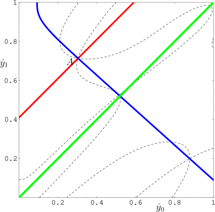
Figure 5: Comparison of the analytical solution for y^0subscript^𝑦0\hat{y}_{0} and y^1subscript^𝑦1\hat{y}_{1}, depicted by the intersection of the two solid curves given by (Eq. (3.27)) and (Eq. (3.24)), with the solution obtained by the method of section 2, which are printed dashed. The parameter values are Ac=5.0subscript𝐴𝑐5.0A_{c}=5.0, γ˙^0=0.2subscript^˙𝛾00.2\hat{\dot{\gamma}}_{0}=0.2, γ˙^1=0.8subscript^˙𝛾10.8\hat{\dot{\gamma}}_{1}=0.8, γ˙^=0.5delimited-⟨⟩^˙𝛾0.5\langle\hat{\dot{\gamma}}\rangle=0.5 and D^=0.01^𝐷0.01\hat{D}=0.01. The diagonal curve indicates the line y^1=y^0subscript^𝑦1subscript^𝑦0\hat{y}_{1}=\hat{y}_{0} and physical solutions are in the upper left triangle. The intersection point A𝐴A between the two dashed curves is practically on top of the intersection point of the solid curves (y^0=0.3033subscript^𝑦00.3033\hat{y}_{0}=0.3033,y^1=0.7130subscript^𝑦10.7130\hat{y}_{1}=0.7130).
Refer to caption
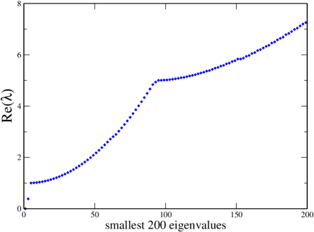
Figure 6: Real parts of the 200 eigenvalues with smallest real parts of the system of equations (3.28) for non-undulating perturbations. The parameter values are Ac=5,y^0=0.4806,y^1=0.6101,γ˙^=0.5,γ˙^0=0.2,γ˙^1=0.8formulae-sequencesubscript𝐴𝑐5formulae-sequencesubscript^𝑦00.4806formulae-sequencesubscript^𝑦10.6101formulae-sequencedelimited-⟨⟩^˙𝛾0.5formulae-sequencesubscript^˙𝛾00.2subscript^˙𝛾10.8A_{c}=5,\hat{y}_{0}=0.4806,\hat{y}_{1}=0.6101,\langle\hat{\dot{\gamma}}\rangle=0.5,\hat{\dot{\gamma}}_{0}=0.2,\hat{\dot{\gamma}}_{1}=0.8, and D^=105^𝐷superscript105\hat{D}=10^{-5}. The smallest eigenvalue is 00, demonstrating that the system is neutrally stable. Eigenvalues are more concentrated around λ=1𝜆1\lambda=1 and λ=5𝜆5\lambda=5 in agreement with the analytical asymptotic result.The first eigenvalue λ=0𝜆0\lambda=0 is related to δΣ^𝛿^Σ\delta\widehat{\Sigma}, the second with λ 0.1𝜆0.1\lambda\,\approx\,0.1 to β1subscript𝛽1\beta_{1} and all eigenvalues λ=1𝜆1\lambda=1 to αnsubscript𝛼𝑛\alpha_{n}, and λ=Ac=5𝜆subscript𝐴𝑐5\lambda=A_{c}=5 to δnsubscript𝛿𝑛\delta_{n}.

In section 2 we demonstrated how to find the stationary state(s) of system defined by Eq. (2.2) graphically as the intersection point(s) of two families of curves, defined by Eqs. (2.17) and (2.18). For the case D^0^𝐷0\hat{D}\to 0, we can actually find an excellent analytic approximation to the stationary solution(s) which is remarkably close to stationary solutions found by the graphical method. In the limit D^0^𝐷0\hat{D}\to 0 equations (2.16) and (2.18) reduce to

αΣ^Acγ˙^0zcos(zD^(y^1y^0))+(γ˙^0αΣ^Ac)Aczsin(zD^(y^1y^0))𝛼^Σsubscript𝐴𝑐subscript^˙𝛾0𝑧𝑧^𝐷subscript^𝑦1subscript^𝑦0subscript^˙𝛾0𝛼^Σsubscript𝐴𝑐subscript𝐴𝑐𝑧𝑧^𝐷subscript^𝑦1subscript^𝑦0\displaystyle\frac{\alpha\widehat{\Sigma}-A_{c}\hat{\dot{\gamma}}_{0}}{z}\cos\left(\sqrt{\frac{z}{\hat{D}}}(\hat{y}_{1}-\hat{y}_{0})\right)+\left(\hat{\dot{\gamma}}_{0}-\frac{\alpha\widehat{\Sigma}}{A_{c}}\right)\sqrt{\frac{A_{c}}{z}}\sin\left(\sqrt{\frac{z}{\hat{D}}}(\hat{y}_{1}-\hat{y}_{0})\right) =(1+αΣ^Acγ˙^0Acγ˙^0γ˙^1)(γ˙^1γ˙^0)absent1𝛼^Σsubscript𝐴𝑐subscript^˙𝛾0subscript𝐴𝑐subscript^˙𝛾0subscript^˙𝛾1subscript^˙𝛾1subscript^˙𝛾0\displaystyle=\left(1+\frac{\alpha\widehat{\Sigma}-A_{c}\hat{\dot{\gamma}}_{0}}{A_{c}\hat{\dot{\gamma}}_{0}-\hat{\dot{\gamma}}_{1}}\right)(\hat{\dot{\gamma}}_{1}-\hat{\dot{\gamma}}_{0}) (3.23a)
αΣ^Acγ˙^0zsin(zD^(y^1y^0))Acz(γ˙^0αΣ^Ac)cos(zD^(y^1y^0))𝛼^Σsubscript𝐴𝑐subscript^˙𝛾0𝑧𝑧^𝐷subscript^𝑦1subscript^𝑦0subscript𝐴𝑐𝑧subscript^˙𝛾0𝛼^Σsubscript𝐴𝑐𝑧^𝐷subscript^𝑦1subscript^𝑦0\displaystyle\frac{\alpha\widehat{\Sigma}-A_{c}\hat{\dot{\gamma}}_{0}}{z}\sin\left(\sqrt{\frac{z}{\hat{D}}}(\hat{y}_{1}-\hat{y}_{0})\right)-\sqrt{\frac{A_{c}}{z}}\left(\hat{\dot{\gamma}}_{0}-\frac{\alpha\widehat{\Sigma}}{A_{c}}\right)\cos\left(\sqrt{\frac{z}{\hat{D}}}(\hat{y}_{1}-\hat{y}_{0})\right) =(γ˙^1αΣ^)z,absentsubscript^˙𝛾1𝛼^Σ𝑧\displaystyle=\frac{(\hat{\dot{\gamma}}_{1}-{\alpha\widehat{\Sigma}})}{\sqrt{z}}, (3.23b)

keeping all terms up to order D^^𝐷\sqrt{\hat{D}}. If we next square Eqs. (3.23a) and (3.23b) and add them we find the following relation

(αΣ^Acγ˙^0αΣ^γ˙^1)2superscript𝛼^Σsubscript𝐴𝑐subscript^˙𝛾0𝛼^Σsubscript^˙𝛾12\displaystyle\left(\frac{\alpha\widehat{\Sigma}-A_{c}\hat{\dot{\gamma}}_{0}}{\alpha\widehat{\Sigma}-\hat{\dot{\gamma}}_{1}}\right)^{2} =Ac(z+1)z+Ac.absentsubscript𝐴𝑐𝑧1𝑧subscript𝐴𝑐\displaystyle=\frac{A_{c}(z+1)}{z+A_{c}}. (3.24)

If we would next substitute the value of Σ^^Σ\widehat{\Sigma} as given by Eq. (A.2), we could express y^1subscript^𝑦1\hat{y}_{1} in terms of y^0subscript^𝑦0\hat{y}_{0}. However, first we obtain the width of the interface, that is the value of y^1y0^subscript^𝑦1^subscript𝑦0\hat{y}_{1}-\hat{y_{0}}, to verify if it scales proportionally to D^^𝐷{\sqrt{\hat{D}}} in agreement with findings in the literature. We therefore solve Eqs. (3.23) for sin(zD^(y^1y^0))𝑧^𝐷subscript^𝑦1subscript^𝑦0\sin\left(\sqrt{\frac{z}{\hat{D}}}(\hat{y}_{1}-\hat{y}_{0})\right) and obtain, after using Eq. (3.24),

sin(zD^(y^1y^0))=Ac+1z+1+Ac+Ac/z.𝑧^𝐷subscript^𝑦1subscript^𝑦0subscript𝐴𝑐1𝑧1subscript𝐴𝑐subscript𝐴𝑐𝑧\displaystyle\sin\left(\sqrt{\frac{z}{\hat{D}}}(\hat{y}_{1}-\hat{y}_{0})\right)=\frac{\sqrt{A_{c}}+1}{\sqrt{z+1+A_{c}+A_{c}/z}}. (3.25)

When we invert this equation we get the following expression for interface width

y^1y^0=D^z((2M+1)πarcsin(Ac+1z+1+Ac+Ac/z)).subscript^𝑦1subscript^𝑦0^𝐷𝑧2𝑀1𝜋subscript𝐴𝑐1𝑧1subscript𝐴𝑐subscript𝐴𝑐𝑧\displaystyle\hat{y}_{1}-\hat{y}_{0}=\sqrt{\frac{\hat{D}}{z}}\left((2M+1)\pi-\arcsin\left(\frac{\sqrt{A_{c}}+1}{\sqrt{z+1+A_{c}+A_{c}/z}}\right)\right). (3.26)

The other solution of Eq. (3.25) is not compatible with the condition γ˙^1<αΣ^<Acγ˙^0subscript^˙𝛾1𝛼^Σsubscript𝐴𝑐subscript^˙𝛾0\hat{\dot{\gamma}}_{1}<\alpha\widehat{\Sigma}<A_{c}\hat{\dot{\gamma}}_{0} and therefore does not correspond to a physical solution. The index M𝑀M is the band index. M=0𝑀0M=0 designates the two band solution (A𝐴A), M=1𝑀1M=1 has two extra bands, like solution B𝐵B, and so on. Expression (3.26) confirms that the interface scales as D^^𝐷\sqrt{\hat{D}}, as observed in olmsted99a ; fielding04 , and gives an exact value for the interface length as a function of z𝑧z and Acsubscript𝐴𝑐A_{c}. An implication of Eq. (3.26) is that shear bands can only exist when D^^𝐷\hat{D} is sufficiently small. Indeed the maximum possible width of the interface is y^1y^01similar-to-or-equalssubscript^𝑦1subscript^𝑦01\hat{y}_{1}-\hat{y}_{0}\simeq 1, implying a maximum value of D^z(π1)2superscript^𝐷𝑧superscript𝜋12\hat{D}^{\ast}\,\approx\,\frac{z}{(\pi-1)^{2}}. In the case we have been considering z=1/3𝑧13z=1/3, and Ac=5subscript𝐴𝑐5A_{c}=5, we find D^0.054similar-to-or-equalssuperscript^𝐷0.054\hat{D}^{\ast}\simeq 0.054, which agrees with our numerical findings. The values of y^0subscript^𝑦0\hat{y}_{0} and y^1subscript^𝑦1\hat{y}_{1} for small D^^𝐷\hat{D} can be determined analytically by using Eq. (3.24) once more, and substituting the expression of αΣ^𝛼superscript^Σ\alpha\widehat{\Sigma}^{\ast} as given in Eq. (A.2) thereby using Eq. (3.26). This calculation gives the following expression for y^0subscript^𝑦0\hat{y}_{0}, which designates the position of the interface of the steady state with 2(M+1)2𝑀12(M+1) shear bands

y^0=[(Ac1)(Acγ˙^0+γ˙^1γ˙^0γ˙^1]((γ˙^1γ˙^)Acγ˙^0+(Acγ˙^0γ˙^)γ˙^1D^(1+(2M+1)πhz)(Ac1)),\displaystyle\hat{y}_{0}=\left[\frac{(A_{c}-1)(\sqrt{A_{c}\hat{\dot{\gamma}}_{0}}+\sqrt{\hat{\dot{\gamma}}_{1}}}{\hat{\dot{\gamma}}_{0}\hat{\dot{\gamma}}_{1}}\right]\left((\hat{\dot{\gamma}}_{1}-\langle\hat{\dot{\gamma}}\rangle)\sqrt{A_{c}\hat{\dot{\gamma}}_{0}}+(A_{c}\hat{\dot{\gamma}}_{0}-\langle\hat{\dot{\gamma}}\rangle)\sqrt{\hat{\dot{\gamma}}_{1}}-\sqrt{{\hat{D}}}\left(1+\frac{(2M+1)\pi-h}{\sqrt{z}}\right)(A_{c}-1)\right), (3.27)

where harcsin(Ac+1z+1+Ac+Ac/z) 0.77subscript𝐴𝑐1𝑧1subscript𝐴𝑐subscript𝐴𝑐𝑧similar-to-or-equals0.77h\,\equiv\,\arcsin\left(\frac{\sqrt{A_{c}}+1}{\sqrt{z+1+A_{c}+A_{c}/z}}\right)\,\simeq\,0.77 for the parameter values used in this paper. From Fig. 5, one can see that the analytical solution (3.27) with M=0𝑀0M=0 found for D^0^𝐷0\hat{D}\to 0, is still an excellent approximation for D^=0.01^𝐷0.01\hat{D}=0.01. The other stationary states with multiple (2(M+1)2𝑀12(M+1)) bands can be found similarly, by substituting the corresponding value of M𝑀M in Eq. (3.27). Note that multiple bands are not present for D^=0.01^𝐷0.01\hat{D}=0.01, as is shown in Fig. 5 where we only find one intersection point (A𝐴A) of the solid curves.

Refer to caption
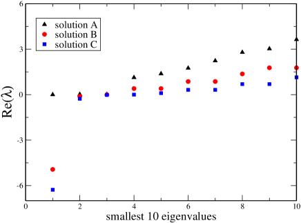
Figure 7: The real part of the first 10 eigenvalues of 𝐒1𝐋𝐑superscript𝐒1superscript𝐋𝐑{\bf S}^{-1}{\bf L^{R}} for an expansion of Eq. (2.1) in n=1000𝑛1000n=1000 modes with zero wave number k𝑘k for solutions A ()(\triangle), B ()(\circ), and C ()(\square). The parameters are the same as in Fig. 3: Ac=5subscript𝐴𝑐5A_{c}=5, γ˙^=0.50delimited-⟨⟩^˙𝛾0.50\langle{\hat{\dot{\gamma}}}\rangle=0.50, and γ˙^0=0.2subscript^˙𝛾00.2\hat{\dot{\gamma}}_{0}=0.2, γ˙^1=0.8subscript^˙𝛾10.8\hat{\dot{\gamma}}_{1}=0.8; the diffusion constant D^=0.001^𝐷0.001\hat{D}=0.001. It can be clearly seen that the real part of the eigenvalues for solutions B and C cross zero, indicating instability of the solutions with multiple bands. Only the solution with two bands (A) is (neutrally) stable.

In order to study the stability of the solutions obeying Eq. (3.26), to non-undulating perturbations we need to determine the eigenvalues of the evolution equations for an(t^)subscript𝑎𝑛^𝑡a_{n}(\hat{t}), bn(t^)subscript𝑏𝑛^𝑡b_{n}(\hat{t}), dn(t^)subscript𝑑𝑛^𝑡d_{n}(\hat{t}) (or equivalently αn(t^)subscript𝛼𝑛^𝑡\alpha_{n}(\hat{t}), βn(t^)subscript𝛽𝑛^𝑡\beta_{n}(\hat{t}), δn(t^)subscript𝛿𝑛^𝑡\delta_{n}(\hat{t})), δγ˙^(y^0,t^)𝛿^˙𝛾subscript^𝑦0^𝑡\delta\hat{\dot{\gamma}}(\hat{y}_{0},\hat{t}), δγ˙^(y^0,t^)𝛿^˙𝛾subscript^𝑦0^𝑡\delta\hat{\dot{\gamma}}(\hat{y}_{0},\hat{t}) and δΣ^(t^)𝛿^Σ^𝑡\delta\widehat{\Sigma}(\hat{t}) for k=0𝑘0k=0. Because the imaginary parts of the governing equations all depend linearly on k𝑘k, we can restrict ourselves to the real part of the differential equations for the amplitudes αnsubscript𝛼𝑛\alpha_{n}, βnsubscript𝛽𝑛\beta_{n}, δnsubscript𝛿𝑛\delta_{n}, δγ˙^(y^0,t^)𝛿^˙𝛾subscript^𝑦0^𝑡\delta\hat{\dot{\gamma}}(\hat{y}_{0},\hat{t}), δγ˙^(y^0,t^)𝛿^˙𝛾subscript^𝑦0^𝑡\delta\hat{\dot{\gamma}}(\hat{y}_{0},\hat{t}) and δΣ^𝛿^Σ\delta\widehat{\Sigma}. These equations can easily be found by projecting out the different sine and cosine modes and are given by Eqs. (B), (B), (B), (B), (B), and (B). For k=0𝑘0k=0 and D^0^𝐷0\hat{D}\to 0 the evolution equations for αn(k,t^)subscript𝛼𝑛𝑘^𝑡\alpha_{n}(k,\hat{t}), βn(k,t^)subscript𝛽𝑛𝑘^𝑡\beta_{n}(k,\hat{t}), δn(k,t^)subscript𝛿𝑛𝑘^𝑡\delta_{n}(k,\hat{t}), δγ˙^(y^0,t^)𝛿^˙𝛾subscript^𝑦0^𝑡\delta\hat{\dot{\gamma}}(\hat{y}_{0},\hat{t}), δγ˙^(y^1,t^)𝛿^˙𝛾subscript^𝑦1^𝑡\delta\hat{\dot{\gamma}}(\hat{y}_{1},\hat{t}) and δΣ^(k,t^)𝛿^Σ𝑘^𝑡\delta\widehat{\Sigma}(k,\hat{t}) read:

dαmdt^dαδΣ^dt^+dδγ˙^(y^0,t^)dt^=Acδγ˙^(y^0,t^)Acαm𝑑subscript𝛼𝑚𝑑^𝑡𝑑𝛼𝛿^Σ𝑑^𝑡𝑑𝛿^˙𝛾subscript^𝑦0^𝑡𝑑^𝑡subscript𝐴𝑐𝛿^˙𝛾subscript^𝑦0^𝑡subscript𝐴𝑐subscript𝛼𝑚\displaystyle\frac{d\alpha_{m}}{d\hat{t}}-\frac{d\alpha\delta\widehat{\Sigma}}{d\hat{t}}+\frac{d\delta\hat{\dot{\gamma}}(\hat{y}_{0},\hat{t})}{d\hat{t}}=-A_{c}\delta\hat{\dot{\gamma}}(\hat{y}_{0},\hat{t})-A_{c}\alpha_{m} (3.28a)
dβmdt^dαδΣ^dt^(1(1)m2)+12dδγ˙^(y^0,t^)dt^(1)m2dδγ˙^(y^1,t^)dt^=z(1m2π2((2M+1)πh)2)βm𝑑subscript𝛽𝑚𝑑^𝑡𝑑𝛼𝛿^Σ𝑑^𝑡1superscript1𝑚212𝑑𝛿^˙𝛾subscript^𝑦0^𝑡𝑑^𝑡superscript1𝑚2𝑑𝛿^˙𝛾subscript^𝑦1^𝑡𝑑^𝑡𝑧1superscript𝑚2superscript𝜋2superscript2𝑀1𝜋2subscript𝛽𝑚\displaystyle\frac{d\beta_{m}}{d\hat{t}}-\frac{d\alpha\delta\widehat{\Sigma}}{d\hat{t}}\left(\frac{1-(-1)^{m}}{2}\right)+\frac{1}{2}\frac{d\delta\hat{\dot{\gamma}}(\hat{y}_{0},\hat{t})}{d\hat{t}}-\frac{(-1)^{m}}{2}\frac{d\delta\hat{\dot{\gamma}}(\hat{y}_{1},\hat{t})}{d\hat{t}}=z\left(1-\frac{m^{2}\pi^{2}}{((2M+1)\pi-h)^{2}}\right)\beta_{m}
+z2δγ˙^(y^0,t^)z(1)m2δγ˙^(y^1,t^)𝑧2𝛿^˙𝛾subscript^𝑦0^𝑡𝑧superscript1𝑚2𝛿^˙𝛾subscript^𝑦1^𝑡\displaystyle+\frac{z}{2}\delta\hat{\dot{\gamma}}(\hat{y}_{0},\hat{t})-\frac{z(-1)^{m}}{2}\delta\hat{\dot{\gamma}}(\hat{y}_{1},\hat{t}) (3.28b)
dδmdt^dαδΣ^dt^+dδγ˙^(y^1,t^)dt^=δγ˙^(y^1,t)δm𝑑subscript𝛿𝑚𝑑^𝑡𝑑𝛼𝛿^Σ𝑑^𝑡𝑑𝛿^˙𝛾subscript^𝑦1^𝑡𝑑^𝑡𝛿^˙𝛾subscript^𝑦1𝑡subscript𝛿𝑚\displaystyle\frac{d\delta_{m}}{d\hat{t}}-\frac{d\alpha\delta\widehat{\Sigma}}{d\hat{t}}+\frac{d\delta\hat{\dot{\gamma}}(\hat{y}_{1},\hat{t})}{d\hat{t}}=-\delta\hat{\dot{\gamma}}(\hat{y}_{1},t)-\delta_{m} (3.28c)
dδγ˙^(y^0,t^)dt^dαδΣ^dt^+n=0dαndt^8(2n+1)2π2=Acδγ˙^(y^0,t^)Acn=08αn(2n+1)2π2𝑑𝛿^˙𝛾subscript^𝑦0^𝑡𝑑^𝑡𝑑𝛼𝛿^Σ𝑑^𝑡superscriptsubscript𝑛0𝑑subscript𝛼𝑛𝑑^𝑡8superscript2𝑛12superscript𝜋2subscript𝐴𝑐𝛿^˙𝛾subscript^𝑦0^𝑡subscript𝐴𝑐superscriptsubscript𝑛08subscript𝛼𝑛superscript2𝑛12superscript𝜋2\displaystyle\frac{d\delta\hat{\dot{\gamma}}(\hat{y}_{0},\hat{t})}{d\hat{t}}-\frac{d\alpha\delta\widehat{\Sigma}}{d\hat{t}}+\sum_{n=0}^{\infty}\frac{d\alpha_{n}}{d\hat{t}}\frac{8}{(2n+1)^{2}\pi^{2}}=-A_{c}\delta\hat{\dot{\gamma}}(\hat{y}_{0},\hat{t})-A_{c}\sum_{n=0}^{\infty}\frac{8\alpha_{n}}{(2n+1)^{2}\pi^{2}} (3.28d)
dδγ˙^(y^1,t^)dt^dαδΣ^dt^+n=0dδndt^8(2n+1)2π2=δγ˙^(y^1,t^)n=08δn(2n+1)2π2𝑑𝛿^˙𝛾subscript^𝑦1^𝑡𝑑^𝑡𝑑𝛼𝛿^Σ𝑑^𝑡superscriptsubscript𝑛0𝑑subscript𝛿𝑛𝑑^𝑡8superscript2𝑛12superscript𝜋2𝛿^˙𝛾subscript^𝑦1^𝑡superscriptsubscript𝑛08subscript𝛿𝑛superscript2𝑛12superscript𝜋2\displaystyle\frac{d\delta\hat{\dot{\gamma}}(\hat{y}_{1},\hat{t})}{d\hat{t}}-\frac{d\alpha\delta\widehat{\Sigma}}{d\hat{t}}+\sum_{n=0}^{\infty}\frac{d\delta_{n}}{d\hat{t}}\frac{8}{(2n+1)^{2}\pi^{2}}=-\delta\hat{\dot{\gamma}}(\hat{y}_{1},\hat{t})-\sum_{n=0}^{\infty}\frac{8\delta_{n}}{(2n+1)^{2}\pi^{2}} (3.28e)
dαδΣ^dt^=Ac(y^0+y^1)δγ˙^(y^0,t^)2+(2y^1y^0)δγ˙^(y^1,t^)2+4Ac(y^0+y^1)n=0αn(2n+1)2π2+4(2y^1y^0)n=0δn(2n+1)2π2.𝑑𝛼𝛿^Σ𝑑^𝑡subscript𝐴𝑐subscript^𝑦0subscript^𝑦1𝛿^˙𝛾subscript^𝑦0^𝑡22subscript^𝑦1subscript^𝑦0𝛿^˙𝛾subscript^𝑦1^𝑡24subscript𝐴𝑐subscript^𝑦0subscript^𝑦1superscriptsubscript𝑛0subscript𝛼𝑛superscript2𝑛12superscript𝜋242subscript^𝑦1subscript^𝑦0superscriptsubscript𝑛0subscript𝛿𝑛superscript2𝑛12superscript𝜋2\displaystyle\frac{d\alpha\delta\widehat{\Sigma}}{d\hat{t}}=A_{c}(\hat{y}_{0}+\hat{y}_{1})\frac{\delta\hat{\dot{\gamma}}(\hat{y}_{0},\hat{t})}{2}+(2-\hat{y}_{1}-\hat{y}_{0})\frac{\delta\hat{\dot{\gamma}}(\hat{y}_{1},\hat{t})}{2}+4A_{c}(\hat{y}_{0}+\hat{y}_{1})\sum_{n=0}^{\infty}\frac{\alpha_{n}}{(2n+1)^{2}\pi^{2}}+4(2-\hat{y}_{1}-\hat{y}_{0})\sum_{n=0}^{\infty}\frac{\delta_{n}}{(2n+1)^{2}\pi^{2}}. (3.28f)

Eqs. (3.28) contain a lot of information. It is immediately clear, for example, that λ=0𝜆0\lambda=0 is an eigenvalue of Eqs. (3.28), by which we mean that solutions with all amplitudes decaying as exp(λt)𝜆𝑡\exp(-\lambda t) with λ=0𝜆0\lambda=0, exist. This can be seen by interpreting Eqs. (3.28) as a matrix equation which has the eigenvalue corresponding to δΣ^𝛿^Σ\delta\widehat{\Sigma} equal to zero,

If it is proved that all amplitudes except dδΣ^dt^=0𝑑𝛿^Σ𝑑^𝑡0\frac{d\delta\widehat{\Sigma}}{d\hat{t}}=0 are always decay, and thus have eigenvalues with positive real parts , we have shown that the shear banded state is neutrally stable. This agrees with Fielding fielding04 and Yih yih . It should also be noticed that the equation for δΣ^𝛿^Σ\delta\widehat{\Sigma} decouples from the other equations as no δΣ^𝛿^Σ\delta\widehat{\Sigma} terms appear in the equations for the other amplitudes and we could therefore elimate all t^δΣ^subscript^𝑡𝛿^Σ\partial_{\hat{t}}\delta\widehat{\Sigma} terms in Eqs. (3.28) by substituting the right-hand side of Eq. (3.28f) for t^δΣ^subscript^𝑡𝛿^Σ\partial_{\hat{t}}\delta\widehat{\Sigma} in first five equations of (3.28). Thus we only need to focus on Eqs. (3.28a-3.28e).

By subtracting Eqs. (3.28d) from (3.28a), we can find an equation expressed entirely in terms of αnsubscript𝛼𝑛\alpha_{n}, and subtracting Eqs. (3.28e) from (3.28c) gives an equation in terms of δnsubscript𝛿𝑛\delta_{n}:

dαmdt^8n=0dαndt^1(2n+1)2π2=Ac[αm8n=0αn(2n+1)2π2],𝑑subscript𝛼𝑚𝑑^𝑡8superscriptsubscript𝑛0𝑑subscript𝛼𝑛𝑑^𝑡1superscript2𝑛12superscript𝜋2subscript𝐴𝑐delimited-[]subscript𝛼𝑚8superscriptsubscript𝑛0subscript𝛼𝑛superscript2𝑛12superscript𝜋2\displaystyle\frac{d\alpha_{m}}{d\hat{t}}-8\sum_{n=0}^{\infty}\frac{d\alpha_{n}}{d\hat{t}}\frac{1}{(2n+1)^{2}\pi^{2}}=-A_{c}\left[\alpha_{m}-8\sum_{n=0}^{\infty}\frac{\alpha_{n}}{(2n+1)^{2}\pi^{2}}\right], (3.29a)
dδmdt^8n=0dδndt^1(2n+1)2π2=[δm8n=0δn(2n+1)2π2].𝑑subscript𝛿𝑚𝑑^𝑡8superscriptsubscript𝑛0𝑑subscript𝛿𝑛𝑑^𝑡1superscript2𝑛12superscript𝜋2delimited-[]subscript𝛿𝑚8superscriptsubscript𝑛0subscript𝛿𝑛superscript2𝑛12superscript𝜋2\displaystyle\frac{d\delta_{m}}{d\hat{t}}-8\sum_{n=0}^{\infty}\frac{d\delta_{n}}{d\hat{t}}\frac{1}{(2n+1)^{2}\pi^{2}}=-\left[\delta_{m}-8\sum_{n=0}^{\infty}\frac{\delta_{n}}{(2n+1)^{2}\pi^{2}}\right]. (3.29b)

The eigenvalues of Eq. (3.29a) are λ=Ac𝜆subscript𝐴𝑐\lambda=A_{c} and of Eq. (3.29b) λ=1𝜆1\lambda=1, reflecting the decay of these amplitudes in time. When we next consider Eqs. (B) and (B) and Eq. (3.28f to eliminate the dδΣ^dt^𝑑𝛿^Σ𝑑^𝑡\frac{d\delta\widehat{\Sigma}}{d\hat{t}} terms, we find that the perturbations in the interface shear stresses obey

dδγ˙^0dt^=Ac(1y^0+y^12)δγ˙^0+(1y^0+y^12)δγ˙^1,𝑑𝛿subscript^˙𝛾0𝑑^𝑡subscript𝐴𝑐1subscript^𝑦0subscript^𝑦12𝛿subscript^˙𝛾01subscript^𝑦0subscript^𝑦12𝛿subscript^˙𝛾1\displaystyle\frac{d\delta\hat{\dot{\gamma}}_{0}}{d\hat{t}}=-A_{c}\left(1-\frac{\hat{y}_{0}+\hat{y}_{1}}{2}\right)\delta\hat{\dot{\gamma}}_{0}+\left(1-\frac{\hat{y}_{0}+\hat{y}_{1}}{2}\right)\delta\hat{\dot{\gamma}}_{1}, (3.30a)
dγ˙^1dt^=(y^0+y^12)γ˙^1+Ac(y^0+y^12)γ˙^0.𝑑subscript^˙𝛾1𝑑^𝑡subscript^𝑦0subscript^𝑦12subscript^˙𝛾1subscript𝐴𝑐subscript^𝑦0subscript^𝑦12subscript^˙𝛾0\displaystyle\frac{d\hat{\dot{\gamma}}_{1}}{d\hat{t}}=-\left(\frac{\hat{y}_{0}+\hat{y}_{1}}{2}\right)\hat{\dot{\gamma}}_{1}+A_{c}\left(\frac{\hat{y}_{0}+\hat{y}_{1}}{2}\right)\hat{\dot{\gamma}}_{0}. (3.30b)

Using Eq. (3.18) with the amplitudes Ansubscript𝐴𝑛A_{n} and Dnsubscript𝐷𝑛D_{n} set to zero, as we have previously found that these decay in time, and neglecting terms of order y^1y^0subscript^𝑦1subscript^𝑦0\hat{y}_{1}-\hat{y}_{0} we readily find that Eqs. (3.30a) and (3.30b) reduce to a single differential equation for γ˙^0subscript^˙𝛾0\hat{\dot{\gamma}}_{0} that reads

dδγ˙^0dt^=Ac(1y^0)δγ˙^0y^0δγ˙^0,𝑑𝛿subscript^˙𝛾0𝑑^𝑡subscript𝐴𝑐1subscript^𝑦0𝛿subscript^˙𝛾0subscript^𝑦0𝛿subscript^˙𝛾0\displaystyle\frac{d\delta\hat{\dot{\gamma}}_{0}}{d\hat{t}}=-A_{c}\left(1-\hat{y}_{0}\right)\delta\hat{\dot{\gamma}}_{0}-\hat{y}_{0}\delta\hat{\dot{\gamma}}_{0}, (3.31)

which clearly corresponds to a solution that decreases in time. As in this approximation δγ˙^1𝛿subscript^˙𝛾1\delta\hat{\dot{\gamma}}_{1} is proportional to δγ˙^0𝛿subscript^˙𝛾0\delta\hat{\dot{\gamma}}_{0} the same holds true for δγ˙^1𝛿subscript^˙𝛾1\delta\hat{\dot{\gamma}}_{1}, showing that the the position of the interface is linearly stable. This means that the stability of Eqs. (3.28) only depends on the properties of the amplitudes βmsubscript𝛽𝑚\beta_{m}. The even and odd modes of the amplitudes βmsubscript𝛽𝑚\beta_{m} satisfy different evolution equations. Using the fact that αnsubscript𝛼𝑛\alpha_{n}, δnsubscript𝛿𝑛\delta_{n} and δγ˙^0𝛿subscript^˙𝛾0\delta\hat{\dot{\gamma}}_{0}, δγ˙^1𝛿subscript^˙𝛾1\delta\hat{\dot{\gamma}}_{1} decay in time, the stability properties of the amplitudes βnsubscript𝛽𝑛\beta_{n} for both odd and even n𝑛n are determined by the equation

dβndt^=z(1n2π2((2M+1)πh)2)βn,𝑑subscript𝛽𝑛𝑑^𝑡𝑧1superscript𝑛2superscript𝜋2superscript2𝑀1𝜋2subscript𝛽𝑛\displaystyle\frac{d\beta_{n}}{d\hat{t}}=z\left(1-\frac{n^{2}\pi^{2}}{((2M+1)\pi-h)^{2}}\right)\beta_{n}, (3.32)

where M𝑀M is the band index. The system of equations (3.32) gives eigenvalues

λn=z(1n2π2((2M+1)πh)2).subscript𝜆𝑛𝑧1superscript𝑛2superscript𝜋2superscript2𝑀1𝜋2\displaystyle\lambda_{n}=-z\left(1-\frac{n^{2}\pi^{2}}{((2M+1)\pi-h)^{2}}\right). (3.33)

As the smallest eigenvalue is λ1subscript𝜆1\lambda_{1}, the sign of this quantity determines the stability of the amplitude of βnsubscript𝛽𝑛\beta_{n} and therefore the stability of the system. For M=0𝑀0M=0, λ1>0subscript𝜆10\lambda_{1}>0, which proves that the two banded solution is neutrally stable: all amplitudes αnsubscript𝛼𝑛\alpha_{n}, βnsubscript𝛽𝑛\beta_{n}, δnsubscript𝛿𝑛\delta_{n}, δγ˙^0𝛿subscript^˙𝛾0\delta\hat{\dot{\gamma}}_{0}, δγ˙^1𝛿subscript^˙𝛾1\delta\hat{\dot{\gamma}}_{1} are decaying in time and αδΣ^𝛼𝛿^Σ\alpha\delta\widehat{\Sigma} is staying constant in time. Multiple banded modes with M=1,2𝑀12M=1,2 all have an eigenvalue λ1<0subscript𝜆10\lambda_{1}<0, which indicates instability of these modes.

In conclusion we have proved that for small D^^𝐷\hat{D} the stationary shear band solution, with two bands is neutrally stable against non undulating perturbations and all other stationary states are unstable. Our analytical findings can be verified numerically. In Fig. 6 the results of a numerical calculation of the 200 eigenvalues with smallest real part are displayed, for D^=105^𝐷superscript105\hat{D}=10^{-5}. Besides the zero eigenvalue corresponding to δΣ^𝛿^Σ\delta\widehat{\Sigma}, we indeed find λ=Ac𝜆subscript𝐴𝑐\lambda=A_{c} corresponding to the amplitudes αnsubscript𝛼𝑛\alpha_{n}, and λ=1𝜆1\lambda=1 corresponding to the amplitudes δnsubscript𝛿𝑛\delta_{n}, many times. The degeneracy is lifted by the small, but finite value of D^^𝐷\hat{D} and the finite size of the matrix. The eigenvalue λ 0.1𝜆0.1\lambda\,\approx\,0.1 corresponds to β1subscript𝛽1\beta_{1}. To check our result that all multiple bands solutions are unstable, we numerically calculated the smallest eigenvalues of Eqs. (3.28) for the solutions B𝐵B and C𝐶C, found in section 2. We indeed find that solutions B𝐵B and C𝐶C are unstable to small nonundulating perturbations. This is shown in the graph in Fig. 7, where an eigenvalue with real part smaller than zero was found for both solutions B𝐵B and C𝐶C.

We next turn to the general case in which the diffusion is no longer assumed to vanish and undulations in the perturbations are admitted.

3.4 Linear stability: nonzero diffusion

The linear stability of the stationary solutions found in section 2 with respect to undulatory perturbations are examined numerically. We follow the same strategy as in the previous section, projecting out the different sine and cosine modes, but this time keeping the imaginary parts of the evolution equations (3.17) as k𝑘k is no longer presumed to vanish.

It again proves beneficial to use the scaled amplitudes αn(k,t^)subscript𝛼𝑛𝑘^𝑡\alpha_{n}(k,\hat{t}), βn(k,t^)subscript𝛽𝑛𝑘^𝑡\beta_{n}(k,\hat{t}), δn(k,t^)subscript𝛿𝑛𝑘^𝑡\delta_{n}(k,\hat{t}) defined in Eq. (3.20) rather than the amplitudes an(k,t^)subscript𝑎𝑛𝑘^𝑡a_{n}(k,\hat{t}), bn(k,t^)subscript𝑏𝑛𝑘^𝑡b_{n}(k,\hat{t}), dn(k,t^)subscript𝑑𝑛𝑘^𝑡d_{n}(k,\hat{t}), for numerical convenience. Once we have projected out the sine and cosine modes, we are left with the evolution equations of the amplitudes. The details of this calculation are relegated to Appendix B. Here we merely note that the general structure of the system of differential equations, whose stability we would like to explore can easily be captured in a matrix equation.

By introducing a vector u=(α0,,αn,β1,,βn,δ0,,δn,δγ˙^0,δγ˙^1,δΣ^)𝑢subscript𝛼0subscript𝛼𝑛subscript𝛽1subscript𝛽𝑛subscript𝛿0subscript𝛿𝑛𝛿subscript^˙𝛾0𝛿subscript^˙𝛾1𝛿^Σ{\vec{u}}=(\alpha_{0},\cdots,\alpha_{n},\beta_{1},\cdots,\beta_{n},\delta_{0},\cdots,\delta_{n},\delta\hat{\dot{\gamma}}_{0},\delta\hat{\dot{\gamma}}_{1},\delta\widehat{\Sigma}), the matrix equivalent of the amplitude evolution is given by

𝐒dudt=(𝐋𝐑2ik𝐋𝐈)u,𝐒𝑑𝑢𝑑𝑡superscript𝐋𝐑2𝑖𝑘superscript𝐋𝐈𝑢{\bf S}\cdot\frac{d\vec{u}}{dt}=-({\bf L^{R}}-2ik{\bf L^{I}})\cdot{\vec{u}}, (3.34)

where the (3n+5)×(3n+5)3𝑛53𝑛5(3n+5)\times(3n+5) matrices 𝐒𝐒{\bf S} and 𝐋𝐑,𝐋𝐈superscript𝐋𝐑superscript𝐋𝐈{\bf L^{R}},{\bf L^{I}} can be easily read off from the amplitude equations (B-B) in Appendix B. As in the previous section eigenvalues of the matrix 𝐒1𝐋~𝐒1𝐋𝐑2ik𝐒1𝐋𝐈superscript𝐒1~𝐋superscript𝐒1superscript𝐋𝐑2𝑖𝑘superscript𝐒1superscript𝐋𝐈{\bf S}^{-1}{\bf\tilde{L}}\,{\equiv}\,{\bf S}^{-1}{\bf L^{R}}-2ik{\bf S}^{-1}{\bf L^{I}} with positive real part correspond to stable solutions. The linear stability of the stationary solutions found in section 3.3 with respect to non-undulatory perturbations is retrieved by setting k=0𝑘0k=0 in Eq, (3.34)

The results of the numerical calculations that were performed for this special case are presented in Figs. 6 and 7 show good agreement with the analytical estimate for D^0^𝐷0\hat{D}\to 0 and k=0𝑘0k=0. The general case for k0𝑘0k{\neq}0 does not allow any tractable analytical expressions for the eigenvalues. We therefore have to resort to numerical methods.
Refer to caption
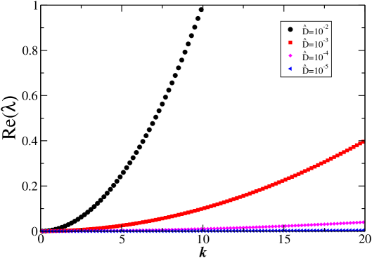
Figure 8: The eigenvalue with smallest real part as a function of k𝑘k for solution A𝐴A using different values of the diffusion constant D^^𝐷\hat{D}. The eigenvalue with smallest real part is observed to increase quadratically with k𝑘k. Moreover, the eigenvalues decrease with decreasing D^^𝐷\hat{D}, eventually approaching zero, a signal of neutral stability.

To find the real part of eigenvalues for the stationary solution A𝐴A, we diagonalize the matrix 𝐋~~𝐋\tilde{\bf L} numerically using the QR algorithm from Ref. numC . We verified our results with the LAPACK linear algebra package lapack , and verified convergence of the eigenvalues up to n=1000𝑛1000n=1000.

Figure 8 shows the real part of the least stable eigenvalue, i.e. that with smallest real part, as a function of k𝑘k. The dependence on k𝑘k is quadratic and for k=0𝑘0k=0 the smallest eigenvalue is equal to 0. The stability decreases with decreasing D^^𝐷\hat{D}; for D^^𝐷\hat{D} decreasing, at a fixed value of k=10𝑘10k=10, from D^=102^𝐷superscript102\hat{D}=10^{-2} to D^=105^𝐷superscript105\hat{D}=10^{-5}, Re(λ)Re𝜆{\rm Re}(\lambda) changes from 1.0 to about 103superscript10310^{-3}.

Refer to caption
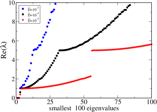
Figure 9: The distribution of the first 100 eigenvalues with smallest real part for fixed k=3𝑘3k=3 and different values of the diffusion constant D^^𝐷\hat{D}. The stair case is clearly recognizable and a clear accumulation of eigenvalues occurs at Re(λ)=1Re𝜆1{\rm Re}(\lambda)=1 and Re(λ)=Ac=5Re𝜆subscript𝐴𝑐5{\rm Re}(\lambda)=A_{c}=5.

To investigate the distribution of eigenvalues, we plot the 100 eigenvalues with the smallest real parts for fixed k=3𝑘3k=3 in Fig. 9. One can still clearly distinguish the plateaus at Re(λ)=1Re𝜆1{\rm Re}(\lambda)=1 and Re(λ)=Ac=5Re𝜆subscript𝐴𝑐5{\rm Re}(\lambda)=A_{c}=5. The plateaus become smaller for increasing D𝐷D, as the eigenvalues increase more rapidly for larger D^^𝐷\hat{D}.

To verify our calculations, we have performed the same calculations for the smooth model originally introduced in Eq. (2.3) (see Appendix C for details). We find that the smooth model, indeed qualitatively reproduces the numerical results of the piecewise toy model.
Refer to caption
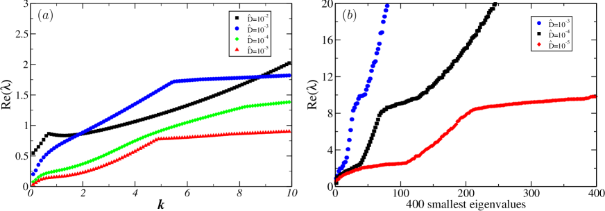
Figure 10: Real part of the eigenvalue with the smallest real part, as a function of the undulation wave number k𝑘k for four different values of the diffusion constant D^^𝐷\hat{D} for the continuous model (a). For small k<1𝑘1k<1 the dependence of Re(λ)Re𝜆{\rm Re}(\lambda) is again approximately quadratic. For larger k𝑘k bumps occur, which are probably caused by the fact that the imaginary part of the equations start to dominate the eigenvalues. The distribution of 400 eigenvalues with smallest real part (b) for k=3𝑘3k=3 is very similar to the distribution obtained by the piecewise toy model of Fig. 9.

Moreover, for this model the shear banding state with two bands is also linearly stable with respect to undulations, as witnessed by the positivity of the real parts of the eigenvalues in Fig. 10. Although we report here only the results Ac=5subscript𝐴𝑐5A_{c}=5, we verified linear stability of the two-band solution for a large number of values of Ac[1,10]subscript𝐴𝑐110A_{c}\in[1,10]. This agrees with the picture that arose from our analytical study for the case of zero diffusion, where we found that one eigenvalue is equal to zero whereas the others are concentrated at Acsubscript𝐴𝑐A_{c} and 111. The effect of diffusion is to shorten the plateaus where eigenvalues have real part 111 or Acsubscript𝐴𝑐A_{c}, and this behavior persists for the entire range of Acsubscript𝐴𝑐A_{c} studied.

The continuous (Fig. 10(a)) and piecewise (Fig. 8) models display qualitatively similar features: the curves initially increase roughly quadratically with k𝑘k and are always positive. For larger k𝑘k values we find Re(λ)ksimilar-toRe𝜆𝑘{\rm Re}(\lambda)\sim k, which suggests that for this k𝑘k regime the imaginary components of the evolution of the amplitudes dominate; and for still larger values of k𝑘k the dependence of Re(λ)(k)Re𝜆𝑘{\rm Re}(\lambda)(k) levels off. This feature was occurs in the piecewise model at much larger k𝑘k-values not shown in Fig. 8. In both cases smaller D^^𝐷\hat{D} gives rise to less stable eigenvalues. Precise comparison between the two models is difficult as the wavenumber k𝑘k is scaled with a factor α=20𝛼20\alpha=20 in the continuous case. This parameter α𝛼\alpha is necessary in order to find a stable shear banding solution in the continuous case SYC96 . One striking difference between the curves in Fig. 8 and Fig. 10(a) is the behavior in the limit k0𝑘0k\to 0. In the smooth model with k0𝑘0k\to 0 the smallest eigenvalue depends on D^^𝐷\hat{D}. The eigenvalue 0 results only when D^0^𝐷0\hat{D}\to 0, in contrast to the piecewise model which is always neutrally stable with respect to non-undulatory perturbations. This can mathematically be understood from the fact that the interface width scales as D^^𝐷\sqrt{\hat{D}} for D^0^𝐷0\hat{D}\to 0. Therefore the matching at the interface can be done in a smoother fashion when D^^𝐷\hat{D} becomes increasingly smaller. In the limit D^0^𝐷0\hat{D}\to 0 this will result in a solution to the piecewise model which approximates the solution to the smooth model. If we compare Fig. 10(b) with Fig. 9, we see the same qualitative behavior. Again plateaus occur, but because of the smoothness of the model the curves are more regular than those obtained for the piecewise toy model. Nevertheless, Fig. 10 suggests that the results for the piecewise model are generic and also valid for general smooth models without normal stresses.

From our findings we therefore conclude that normal stresses are generically responsible for rendering the Johnson-Segalman model linearly unstable for long wavelength undulations. This confirms the results which were first conjectured in Refs. fielding04 ; WilsonFielding2006 .

4 Discussion

We have studied, to a large extent analytically, a toy model for shear banding without normal stresses, but with spatial gradient terms (stress diffusion). We captured the general characteristics of a nonmonotonic stress-shear rate relation by introducing a piecewise linear stress-shear rate curve, which makes analytical calculations tractable. The results obtained for the piecewise model were shown to be in qualitatively agreement from those obtained using a smooth function g𝑔g.

For the set of parameters chosen, we found multiple stationary solutions when D^<102^𝐷superscript102\hat{D}<10^{-2}. For D^=103^𝐷superscript103\hat{D}=10^{-3} we obtain three stationary states: one being the commonly observed two-band profile and the other two having three and four bands. The two-band profile was shown to be linearly stable with respect to two-dimensional undulations. The linear stability of the two-band profile is at variance with analogous results for Johnson-Segalman (JS) model, which was shown by Fielding to have linear instabilities for a certain range of k𝑘k vectors SMF2005 with k 1𝑘1k\,\approx\,1. This strongly suggests that normal stresses, absent in our model, are responsible for the linear instabilities arising in the JS model. Related recent work by Fielding and co-workers fielding06 ; WilsonFielding2006 showed that these linear instabilities are suppressed if nonlinear effects are taken into account. It might be that nonlinear perturbations induce instabilities in the scalar model studied here. The behavior of such (weakly) nonlinear instabilities is a subject of interest and future research.

Acknowledgements

It is a pleasure to thank the British Council and NWO for financial assistance. This work is part of the research programme of the ‘Stichting voor Fundamenteel Onderzoek der Materie (FOM)’, which is financially supported by the ‘Nederlandse Organisatie voor Wetenschappelijk Onderzoek (NWO)’.

Appendix A Integration Constants

The integration constants c1subscript𝑐1c_{1},c2subscript𝑐2c_{2}, d1subscript𝑑1d_{1}, d2subscript𝑑2d_{2} can be expressed in terms of y^0subscript^𝑦0\hat{y}_{0}, the spatial position at which γ˙^^˙𝛾\hat{\dot{\gamma}} equals γ˙^0subscript^˙𝛾0\hat{\dot{\gamma}}_{0}. From the four equations (2.15-2.16) we find

c1subscript𝑐1\displaystyle c_{1} =γ˙^0αΣ^Accosh(AcD^y^0)absentsubscript^˙𝛾0𝛼^Σsubscript𝐴𝑐subscript𝐴𝑐^𝐷subscript^𝑦0\displaystyle=\frac{\hat{\dot{\gamma}}_{0}-\frac{\alpha\widehat{\Sigma}}{A_{c}}}{\cosh\left(\sqrt{\frac{A_{c}}{\hat{D}}}\hat{y}_{0}\right)} (A.1a)
c2subscript𝑐2\displaystyle c_{2} =γ˙^1αΣ^cosh[(y^11)/D^]absentsubscript^˙𝛾1𝛼^Σsubscript^𝑦11^𝐷\displaystyle={\frac{\hat{\dot{\gamma}}_{1}-\alpha\widehat{\Sigma}}{\cosh\left[(\hat{y}_{1}-1)/\sqrt{\hat{D}}\right]}} (A.1b)
d1subscript𝑑1\displaystyle d_{1} =(αΣ^Acγ˙^0)cos(zD^y^0)ztanh(AcD^y^0)sin(zD^y^0)(Acγ˙^0αΣ^)Aczabsent𝛼^Σsubscript𝐴𝑐subscript^˙𝛾0𝑧^𝐷subscript^𝑦0𝑧subscript𝐴𝑐^𝐷subscript^𝑦0𝑧^𝐷subscript^𝑦0subscript𝐴𝑐subscript^˙𝛾0𝛼^Σsubscript𝐴𝑐𝑧\displaystyle=\frac{(\alpha\widehat{\Sigma}-A_{c}\hat{\dot{\gamma}}_{0})\cos\left(\sqrt{\frac{z}{\hat{D}}}\hat{y}_{0}\right)}{z}-\frac{\tanh\left(\sqrt{\frac{A_{c}}{\hat{D}}}\hat{y}_{0}\right)\sin\left(\sqrt{\frac{z}{\hat{D}}}\hat{y}_{0}\right)(A_{c}\hat{\dot{\gamma}}_{0}-\alpha\widehat{\Sigma})}{\sqrt{A_{c}z}} (A.1c)
d2subscript𝑑2\displaystyle d_{2} =(αΣ^Acγ˙^0)sin(zD^y^0)z+tanh(AcD^y^0)cos(zD^y^0)(Acγ˙^0αΣ^)Acz,absent𝛼^Σsubscript𝐴𝑐subscript^˙𝛾0𝑧^𝐷subscript^𝑦0𝑧subscript𝐴𝑐^𝐷subscript^𝑦0𝑧^𝐷subscript^𝑦0subscript𝐴𝑐subscript^˙𝛾0𝛼^Σsubscript𝐴𝑐𝑧\displaystyle=\frac{(\alpha\widehat{\Sigma}-A_{c}\hat{\dot{\gamma}}_{0})\sin\left(\sqrt{\frac{z}{\hat{D}}}\hat{y}_{0}\right)}{z}+\frac{\tanh\left(\sqrt{\frac{A_{c}}{\hat{D}}}\hat{y}_{0}\right)\cos\left(\sqrt{\frac{z}{\hat{D}}}\hat{y}_{0}\right)(A_{c}\hat{\dot{\gamma}}_{0}-\alpha\widehat{\Sigma})}{\sqrt{A_{c}z}}, (A.1d)

where z=Acγ˙^0γ˙^1γ˙^1γ˙^0𝑧subscript𝐴𝑐subscript^˙𝛾0subscript^˙𝛾1subscript^˙𝛾1subscript^˙𝛾0z=\frac{A_{c}\hat{\dot{\gamma}}_{0}-\hat{\dot{\gamma}}_{1}}{\hat{\dot{\gamma}}_{1}-\hat{\dot{\gamma}}_{0}}. From these equations, together with Eqs. (2.17-2.18), the values of y^0subscript^𝑦0\hat{y}_{0} and y^1subscript^𝑦1\hat{y}_{1} can in principle be determined as a function of Σ^^Σ\widehat{\Sigma}. To fix the value of the selected stress Σ^superscript^Σ\widehat{\Sigma}^{\ast} an additional equation is required. From the global constraint of an imposed average shear rate γ˙^delimited-⟨⟩^˙𝛾\langle\hat{\dot{\gamma}}\rangle we can find an expression for Σ^superscript^Σ\widehat{\Sigma}^{\ast}. We substitute Equations (A.1) for the constants c1,2subscript𝑐12c_{1,2} and d1,2subscript𝑑12d_{1,2} into Eqs. (2.14a-2.14c), and calculate the average value of the shear rate directly by splitting up the integral in three parts: [0,y^0]0subscript^𝑦0[0,\hat{y}_{0}],[y^0,y^1]subscript^𝑦0subscript^𝑦1[\hat{y}_{0},\hat{y}_{1}], [y^1,1]subscript^𝑦11[\hat{y}_{1},1]. By equating the sum of the three parts to γ˙^delimited-⟨⟩^˙𝛾\langle{\hat{\dot{\gamma}}}\rangle, we obtain the following expression for Σ^^Σ\widehat{\Sigma} in terms of y^0,y^1subscript^𝑦0subscript^𝑦1\hat{y}_{0},\hat{y}_{1}, γ˙^delimited-⟨⟩^˙𝛾\langle{\hat{\dot{\gamma}}}\rangle, and γ˙^0,γ˙^1subscript^˙𝛾0subscript^˙𝛾1\hat{\dot{\gamma}}_{0},\hat{\dot{\gamma}}_{1}:

αΣ^=Ac{γ˙^0(Ac+z)(y^0y^1)D^[γ˙^0tanh(AcD^y^0)(Ac+zAc)+γ˙^1tanh(1y^1D^)(z+1)]+γ˙^z}Ac(y^0y^1+zzy^1)+y^0zD^[tanh(AcD^y^0)(Ac+zAc)+Ac(1+z)tanh(1y^1D^)].𝛼superscript^Σsubscript𝐴𝑐subscript^˙𝛾0subscript𝐴𝑐𝑧subscript^𝑦0subscript^𝑦1^𝐷delimited-[]subscript^˙𝛾0subscript𝐴𝑐^𝐷subscript^𝑦0subscript𝐴𝑐𝑧subscript𝐴𝑐subscript^˙𝛾11subscript^𝑦1^𝐷𝑧1delimited-⟨⟩^˙𝛾𝑧subscript𝐴𝑐subscript^𝑦0subscript^𝑦1𝑧𝑧subscript^𝑦1subscript^𝑦0𝑧^𝐷delimited-[]subscript𝐴𝑐^𝐷subscript^𝑦0subscript𝐴𝑐𝑧subscript𝐴𝑐subscript𝐴𝑐1𝑧1subscript^𝑦1^𝐷\displaystyle\alpha\widehat{\Sigma}^{\ast}=\frac{A_{c}\left\{\hat{\dot{\gamma}}_{0}(A_{c}+z)(\hat{y}_{0}-\hat{y}_{1})-\sqrt{\hat{D}}\left[\hat{\dot{\gamma}}_{0}\tanh\left(\sqrt{\frac{A_{c}}{\hat{D}}}\hat{y}_{0}\right)\left(\frac{{A_{c}}+z}{\sqrt{A_{c}}}\right)+\hat{\dot{\gamma}}_{1}\tanh\left(\frac{1-\hat{y}_{1}}{\sqrt{\hat{D}}}\right)\left(z+1\right)\right]+{\langle{\hat{\dot{\gamma}}}\rangle}z\right\}}{A_{c}(\hat{y}_{0}-\hat{y}_{1}+z-z\hat{y}_{1})+\hat{y}_{0}z-\sqrt{\hat{D}}\left[\tanh\left(\sqrt{\frac{A_{c}}{\hat{D}}}\hat{y}_{0}\right)\left(\frac{{A_{c}}+z}{\sqrt{A_{c}}}\right)+A_{c}(1+z)\tanh\left(\frac{1-\hat{y}_{1}}{\sqrt{\hat{D}}}\right)\right]}. (A.2)

Appendix B Amplitude evolution equations

The time evolution of the amplitudes αn(k,t^)subscript𝛼𝑛𝑘^𝑡\alpha_{n}(k,\hat{t}) and δγ˙^0(k,t^)𝛿subscript^˙𝛾0𝑘^𝑡\delta\hat{\dot{\gamma}}_{0}(k,\hat{t}) can be determined by substituting δγ˙^I(x^,y^,t^)𝛿superscript^˙𝛾𝐼^𝑥^𝑦^𝑡\delta\hat{\dot{\gamma}}^{I}(\hat{x},\hat{y},\hat{t}) in Eq. (3.12a). When we project out the cosine modes and use the definition of the scaled amplitudes αn(k,t^)=an(k,t^)(2n+1)π(1)n/4subscript𝛼𝑛𝑘^𝑡subscript𝑎𝑛𝑘^𝑡2𝑛1𝜋superscript1𝑛4\alpha_{n}(k,\hat{t})=a_{n}(k,\hat{t})(2n+1)\pi(-1)^{n}/4, we obtain

dαmdt^(γ˙^1Dy^)y^0t^δy^0(k,t^)t^αδΣ^(k,t^)=(Ac+D^k2)(γ˙^1Dy^)y^0δy^0(k,t^)(Ac+D^k2+D^(π(2m+1)2y^0)2)αm𝑑subscript𝛼𝑚𝑑^𝑡subscriptsuperscript^˙𝛾1𝐷^𝑦subscript^𝑦0subscript^𝑡𝛿subscript^𝑦0𝑘^𝑡subscript^𝑡𝛼𝛿^Σ𝑘^𝑡subscript𝐴𝑐^𝐷superscript𝑘2subscriptsuperscript^˙𝛾1𝐷^𝑦subscript^𝑦0𝛿subscript^𝑦0𝑘^𝑡subscript𝐴𝑐^𝐷superscript𝑘2^𝐷superscript𝜋2𝑚12subscript^𝑦02subscript𝛼𝑚\displaystyle\frac{d\alpha_{m}}{d\hat{t}}-\left(\frac{\partial\hat{\dot{\gamma}}^{1D}}{\partial\hat{y}}\right)_{\hat{y}_{0}}\partial_{\hat{t}}\delta\hat{y}_{0}(k,\hat{t})-\partial_{\hat{t}}\alpha\delta\widehat{\Sigma}(k,\hat{t})=(A_{c}+\hat{D}k^{2})\left(\frac{\partial\hat{\dot{\gamma}}^{1D}}{\partial\hat{y}}\right)_{\hat{y}_{0}}\delta\hat{y}_{0}(k,\hat{t})-\left(A_{c}+\hat{D}k^{2}+\hat{D}\left(\frac{\pi(2m+1)}{2\hat{y}_{0}}\right)^{2}\right)\alpha_{m}
+D^k2αΣ^(k,t^)ik(1)m(2m+1)π2y^0[n=1αn(1)n16y^02(2n+1)3π3[RmnATmA]+(γ˙^1Dy^0)y^0δy^0(k,t^)FmA\displaystyle+\hat{D}k^{2}\alpha\widehat{\Sigma}(k,\hat{t})-\frac{ik(-1)^{m}(2m+1)\pi}{2\hat{y}_{0}}\left[\sum_{n=1}^{\infty}\alpha_{n}(-1)^{n}\frac{16\hat{y}_{0}^{2}}{(2n+1)^{3}\pi^{3}}\left[R^{A}_{mn}-T^{A}_{m}\right]+\left(\frac{\partial\hat{\dot{\gamma}}^{1D}}{\partial\hat{y}_{0}}\right)_{\hat{y}_{0}}\delta\hat{y}_{0}(k,\hat{t})F^{A}_{m}\right.
+n=1[LmnA+DAcRmnA]4αn(1)n(2n+1)π(JmA+D^AcTmA)[αδΣ^+(γ˙^1Dy^)y^0δy^0(k,t^)]].\displaystyle+\left.\sum_{n=1}^{\infty}\left[L^{A}_{mn}+\frac{D}{A_{c}}R^{A}_{mn}\right]\frac{4\alpha_{n}(-1)^{n}}{(2n+1)\pi}-\left(J^{A}_{m}+\frac{\hat{D}}{A_{c}}T^{A}_{m}\right)\left[\alpha\delta\widehat{\Sigma}+\left(\frac{\partial\hat{\dot{\gamma}}^{1D}}{\partial\hat{y}}\right)_{\hat{y}_{0}}\delta\hat{y}_{0}(k,\hat{t})\right]\right]. (B.1)
8n=0dαndt^1(2n+1)2π2αt^δΣ^+t^δγ^0=D^k2αδΣ^(Ac+D^k2)δγ^08(Ac+D^k2)n=0αn(2n+1)2π22D^y^02n=0αn8superscriptsubscript𝑛0𝑑subscript𝛼𝑛𝑑^𝑡1superscript2𝑛12superscript𝜋2𝛼subscript^𝑡𝛿^Σsubscript^𝑡𝛿subscript^𝛾0^𝐷superscript𝑘2𝛼𝛿^Σsubscript𝐴𝑐^𝐷superscript𝑘2𝛿subscript^𝛾08subscript𝐴𝑐^𝐷superscript𝑘2superscriptsubscript𝑛0subscript𝛼𝑛superscript2𝑛12superscript𝜋22^𝐷superscriptsubscript^𝑦02superscriptsubscript𝑛0subscript𝛼𝑛\displaystyle 8\sum_{n=0}^{\infty}\frac{d\alpha_{n}}{d\hat{t}}\frac{1}{(2n+1)^{2}\pi^{2}}-\alpha\partial_{\hat{t}}\delta\widehat{\Sigma}+\partial_{\hat{t}}\delta\hat{\gamma}_{0}=\hat{D}k^{2}\alpha\delta\widehat{\Sigma}-(A_{c}+\hat{D}k^{2})\delta\hat{\gamma}_{0}-8(A_{c}+\hat{D}k^{2})\sum_{n=0}^{\infty}\frac{\alpha_{n}}{(2n+1)^{2}\pi^{2}}-\frac{2\hat{D}}{\hat{y}_{0}^{2}}\sum_{n=0}^{\infty}\alpha_{n}
iky^0{n=0αn(1(1)n)16y^02(2n+1)3π3γ˙^0+n=08y^0αn(2n+1)2π2[αΣ^y^0Ac+(γ˙^0αΣ^Ac)D^]\displaystyle-\frac{ik}{\hat{y}_{0}}\left\{-\sum_{n=0}^{\infty}\frac{\alpha_{n}(1-(-1)^{n})16\hat{y}_{0}^{2}}{(2n+1)^{3}\pi^{3}}\hat{\dot{\gamma}}_{0}+\sum_{n=0}^{\infty}\frac{8\hat{y}_{0}\alpha_{n}}{(2n+1)^{2}\pi^{2}}\left[\frac{\alpha\widehat{\Sigma}\hat{y}_{0}}{A_{c}}+(\hat{\dot{\gamma}}_{0}-\frac{\alpha\widehat{\Sigma}}{A_{c}})\sqrt{\hat{D}}\right]\right.
αδΣ^[αΣ^y^022Ac+(γ˙^0αΣ^Ac)D^Ac]+y^0δγ0(αΣ^y^0Ac+(γ˙^0αΣ^Ac)D^)y^02γ˙^0δγ02}\displaystyle-\left.\alpha\delta\widehat{\Sigma}\left[\frac{\alpha\widehat{\Sigma}\hat{y}_{0}^{2}}{2A_{c}}+(\hat{\dot{\gamma}}_{0}-\frac{\alpha\widehat{\Sigma}}{A_{c}})\frac{\hat{D}}{A_{c}}\right]+\hat{y}_{0}\delta\gamma_{0}\left(\frac{\alpha\widehat{\Sigma}\hat{y}_{0}}{A_{c}}+\left(\hat{\dot{\gamma}}_{0}-\frac{\alpha\widehat{\Sigma}}{A_{c}}\right)\sqrt{\hat{D}}\right)-\frac{\hat{y}_{0}^{2}\hat{\dot{\gamma}}_{0}\delta\gamma_{0}}{2}\right\}
D^k2αδΣ^(Ac+D^k2)δγ^08(Ac+D^k2)n=0αn(2n+1)2π22D^y^02n=0αniky^0Π1(k,t^).absent^𝐷superscript𝑘2𝛼𝛿^Σsubscript𝐴𝑐^𝐷superscript𝑘2𝛿subscript^𝛾08subscript𝐴𝑐^𝐷superscript𝑘2superscriptsubscript𝑛0subscript𝛼𝑛superscript2𝑛12superscript𝜋22^𝐷superscriptsubscript^𝑦02superscriptsubscript𝑛0subscript𝛼𝑛𝑖𝑘subscript^𝑦0subscriptΠ1𝑘^𝑡\displaystyle\equiv\hat{D}k^{2}\alpha\delta\widehat{\Sigma}-(A_{c}+\hat{D}k^{2})\delta\hat{\gamma}_{0}-8(A_{c}+\hat{D}k^{2})\sum_{n=0}^{\infty}\frac{\alpha_{n}}{(2n+1)^{2}\pi^{2}}-\frac{2\hat{D}}{\hat{y}_{0}^{2}}\sum_{n=0}^{\infty}\alpha_{n}-\frac{ik}{\hat{y}_{0}}\Pi_{1}(k,\hat{t}). (B.2)

In Eq. (B) we defined the real function Π1(k,t^)subscriptΠ1𝑘^𝑡\Pi_{1}(k,\hat{t}) as the imaginary contribution to the evolution of δγ^0𝛿subscript^𝛾0\delta\hat{\gamma}_{0}. The coefficients RmnA,TmA,FmA,LmnA,JmAsuperscriptsubscript𝑅𝑚𝑛𝐴superscriptsubscript𝑇𝑚𝐴subscriptsuperscript𝐹𝐴𝑚superscriptsubscript𝐿𝑚𝑛𝐴subscriptsuperscript𝐽𝐴𝑚R_{mn}^{A},T_{m}^{A},F^{A}_{m},L_{mn}^{A},J^{A}_{m} in Eqs. (B) are defined in terms of integrals of functions on the interval [0,y^0]0subscript^𝑦0[0,\hat{y}_{0}]:

RmnAsuperscriptsubscript𝑅𝑚𝑛𝐴\displaystyle R_{mn}^{A} =0y^0cos((2m+1)πy^2y^0)cos((2n+1)πy^2y^0)γ˙^1Dy^𝑑y^absentsuperscriptsubscript0subscript^𝑦02𝑚1𝜋^𝑦2subscript^𝑦02𝑛1𝜋^𝑦2subscript^𝑦0superscript^˙𝛾1𝐷^𝑦differential-d^𝑦\displaystyle=\int_{0}^{\hat{y}_{0}}\cos\left(\frac{(2m+1)\pi\hat{y}}{2\hat{y}_{0}}\right)\cos\left(\frac{(2n+1)\pi\hat{y}}{2\hat{y}_{0}}\right)\frac{\partial\hat{\dot{\gamma}}^{1D}}{\partial\hat{y}}\,d\hat{y} (B.3a)
FmAsubscriptsuperscript𝐹𝐴𝑚\displaystyle F^{A}_{m} =0y^0cos((2m+1)πy^2y^0)y^22γ˙^1Dy^𝑑y^absentsuperscriptsubscript0subscript^𝑦02𝑚1𝜋^𝑦2subscript^𝑦0superscript^𝑦22superscript^˙𝛾1𝐷^𝑦differential-d^𝑦\displaystyle=\int_{0}^{\hat{y}_{0}}\cos\left(\frac{(2m+1)\pi\hat{y}}{2\hat{y}_{0}}\right)\frac{\hat{y}^{2}}{2}\frac{\partial\hat{\dot{\gamma}}^{1D}}{\partial\hat{y}}\,d\hat{y} (B.3b)
LmnAsuperscriptsubscript𝐿𝑚𝑛𝐴\displaystyle L_{mn}^{A} =0y^0cos((2m+1)πy^2y^0)cos((2n+1)πy^2y^0)αΣ^y^Ac𝑑y^,absentsuperscriptsubscript0subscript^𝑦02𝑚1𝜋^𝑦2subscript^𝑦02𝑛1𝜋^𝑦2subscript^𝑦0𝛼^Σ^𝑦subscript𝐴𝑐differential-d^𝑦\displaystyle=\int_{0}^{\hat{y}_{0}}\cos\left(\frac{(2m+1)\pi\hat{y}}{2\hat{y}_{0}}\right)\cos\left(\frac{(2n+1)\pi\hat{y}}{2\hat{y}_{0}}\right)\frac{\alpha\widehat{\Sigma}\hat{y}}{A_{c}}\,d\hat{y}, (B.3c)

and TmA=Rm,12Asuperscriptsubscript𝑇𝑚𝐴superscriptsubscript𝑅𝑚12𝐴T_{m}^{A}=R_{m,-\frac{1}{2}}^{A}, and JmA=Lm,12Asubscriptsuperscript𝐽𝐴𝑚superscriptsubscript𝐿𝑚12𝐴J^{A}_{m}=L_{m,-\frac{1}{2}}^{A}. The evolution equations for the amplitudes δn(k,t^)subscript𝛿𝑛𝑘^𝑡\delta_{n}(k,\hat{t}) is derived by substituting the expression for δγ˙^III(x^,y^,t^)𝛿superscript^˙𝛾𝐼𝐼𝐼^𝑥^𝑦^𝑡\delta\hat{\dot{\gamma}}^{III}(\hat{x},\hat{y},\hat{t}) in Eq. (3.12c), projecting out the cosine mode,s and using the scaling relation between dnsubscript𝑑𝑛d_{n} and δnsubscript𝛿𝑛\delta_{n} , yielding

dδmdt^(γ˙^1Dy^)y^1t^δy^1(k,t^)t^αδΣ^(k,t^)=(1+D^k2)(γ˙^1Dy^)y^1δy^1(k,t^)(1+D^k2+D^(π(2m+1)2(1y^1))2)δm𝑑subscript𝛿𝑚𝑑^𝑡subscriptsuperscript^˙𝛾1𝐷^𝑦subscript^𝑦1subscript^𝑡𝛿subscript^𝑦1𝑘^𝑡subscript^𝑡𝛼𝛿^Σ𝑘^𝑡1^𝐷superscript𝑘2subscriptsuperscript^˙𝛾1𝐷^𝑦subscript^𝑦1𝛿subscript^𝑦1𝑘^𝑡1^𝐷superscript𝑘2^𝐷superscript𝜋2𝑚121subscript^𝑦12subscript𝛿𝑚\displaystyle\frac{d\delta_{m}}{d\hat{t}}-\left(\frac{\partial\hat{\dot{\gamma}}^{1D}}{\partial\hat{y}}\right)_{\hat{y}_{1}}\partial_{\hat{t}}\delta\hat{y}_{1}(k,\hat{t})-\partial_{\hat{t}}\alpha\delta\widehat{\Sigma}(k,\hat{t})=(1+\hat{D}k^{2})\left(\frac{\partial\hat{\dot{\gamma}}^{1D}}{\partial\hat{y}}\right)_{\hat{y}_{1}}\delta\hat{y}_{1}(k,\hat{t})-\left(1+\hat{D}k^{2}+\hat{D}\left(\frac{\pi(2m+1)}{2(1-\hat{y}_{1})}\right)^{2}\right)\delta_{m}
+D^k2αΣ^(k,t^)ik(1)m(2m+1)π2(1y^1)[n=1δn(1)n16(1y^1)2(2n+1)3π3[R~mnDT~mD]+(γ˙^1Dy^1)y^1δy^1(k,t^)F~mD\displaystyle+\hat{D}k^{2}\alpha\widehat{\Sigma}(k,\hat{t})-\frac{ik(-1)^{m}(2m+1)\pi}{2(1-\hat{y}_{1})}\left[\sum_{n=1}^{\infty}\delta_{n}(-1)^{n}\frac{16(1-\hat{y}_{1})^{2}}{(2n+1)^{3}\pi^{3}}\left[\tilde{R}^{D}_{mn}-\tilde{T}^{D}_{m}\right]+\left(\frac{\partial\hat{\dot{\gamma}}^{1D}}{\partial\hat{y}_{1}}\right)_{\hat{y}_{1}}\delta\hat{y}_{1}(k,\hat{t})\tilde{F}^{D}_{m}\right.
+n=1[L~mnD+D^R~mnD]4δn(1)n(2n+1)π(J~mD+D^T~mD)[αΣ^+(γ˙^1Dy^)y^1δy^1(k,t^)]]ikγ˙^δm\displaystyle+\left.\sum_{n=1}^{\infty}\left[\tilde{L}^{D}_{mn}+\hat{D}\tilde{R}^{D}_{mn}\right]\frac{4\delta_{n}(-1)^{n}}{(2n+1)\pi}-\left(\tilde{J}^{D}_{m}+\hat{D}\tilde{T}^{D}_{m}\right)\left[\alpha\widehat{\Sigma}+\left(\frac{\partial\hat{\dot{\gamma}}^{1D}}{\partial\hat{y}}\right)_{\hat{y}_{1}}\delta\hat{y}_{1}(k,\hat{t})\right]\right]-ik\langle\hat{\dot{\gamma}}\rangle\delta_{m}
+ik[αδΣ^+(γ˙^1Dy^)y^1δy^1]γ˙^,𝑖𝑘delimited-[]𝛼𝛿^Σsubscriptsuperscript^˙𝛾1𝐷^𝑦subscript^𝑦1𝛿subscript^𝑦1delimited-⟨⟩^˙𝛾\displaystyle+ik\left[\alpha\delta\widehat{\Sigma}+\left(\frac{\partial\hat{\dot{\gamma}}^{1D}}{\partial\hat{y}}\right)_{\hat{y}_{1}}\delta\hat{y}_{1}\right]\langle\hat{\dot{\gamma}}\rangle, (B.4)

where the functions R~mnD,T~mD,F~mD,L~mnD,J~mDsuperscriptsubscript~𝑅𝑚𝑛𝐷superscriptsubscript~𝑇𝑚𝐷subscriptsuperscript~𝐹𝐷𝑚superscriptsubscript~𝐿𝑚𝑛𝐷subscriptsuperscript~𝐽𝐷𝑚\tilde{R}_{mn}^{D},\tilde{T}_{m}^{D},\tilde{F}^{D}_{m},\tilde{L}_{mn}^{D},\tilde{J}^{D}_{m} are defined similarly to Eqs. (B.3), with y^0subscript^𝑦0\hat{y}_{0} everywhere replaced by 1y^11subscript^𝑦11-\hat{y}_{1} and Acsubscript𝐴𝑐A_{c} set to 1. If we integrate the amplitude equation for dn(k,t)subscript𝑑𝑛𝑘𝑡d_{n}(k,t) from y^1subscript^𝑦1\hat{y}_{1} to 111, we obtain the evolution equation for the δγ˙^1(k,t^)𝛿subscript^˙𝛾1𝑘^𝑡\delta\hat{\dot{\gamma}}_{1}(k,\hat{t}),

8n=0dδndt^1(2n+1)2π2αt^δΣ^+t^δγ^1=D^k2αδΣ^(1+D^k2)δγ^18(1+D^k2)n=0δn(2n+1)2π22D^(1y^1)2n=0δn8superscriptsubscript𝑛0𝑑subscript𝛿𝑛𝑑^𝑡1superscript2𝑛12superscript𝜋2𝛼subscript^𝑡𝛿^Σsubscript^𝑡𝛿subscript^𝛾1^𝐷superscript𝑘2𝛼𝛿^Σ1^𝐷superscript𝑘2𝛿subscript^𝛾181^𝐷superscript𝑘2superscriptsubscript𝑛0subscript𝛿𝑛superscript2𝑛12superscript𝜋22^𝐷superscript1subscript^𝑦12superscriptsubscript𝑛0subscript𝛿𝑛\displaystyle 8\sum_{n=0}^{\infty}\frac{d\delta_{n}}{d\hat{t}}\frac{1}{(2n+1)^{2}\pi^{2}}-\alpha\partial_{\hat{t}}\delta\widehat{\Sigma}+\partial_{\hat{t}}\delta\hat{\gamma}_{1}=\hat{D}k^{2}\alpha\delta\widehat{\Sigma}-(1+\hat{D}k^{2})\delta\hat{\gamma}_{1}-8(1+\hat{D}k^{2})\sum_{n=0}^{\infty}\frac{\delta_{n}}{(2n+1)^{2}\pi^{2}}-\frac{2\hat{D}}{(1-\hat{y}_{1})^{2}}\sum_{n=0}^{\infty}\delta_{n}
ik(1y^1){n=0δn(1(1)n)16(1y^1)2(2n+1)3π3γ˙^1+n=08(1y^1)δn(2n+1)2π2[γ˙^+αΣ^(y^11)(γ˙^1αΣ^)D^]\displaystyle-\frac{ik}{(1-\hat{y}_{1})}\left\{-\sum_{n=0}^{\infty}\frac{\delta_{n}(1-(-1)^{n})16(1-\hat{y}_{1})^{2}}{(2n+1)^{3}\pi^{3}}\hat{\dot{\gamma}}_{1}+\sum_{n=0}^{\infty}\frac{8(1-\hat{y}_{1})\delta_{n}}{(2n+1)^{2}\pi^{2}}\left[\langle\hat{\dot{\gamma}}\rangle+\alpha\widehat{\Sigma}(\hat{y}_{1}-1)-(\hat{\dot{\gamma}}_{1}-\alpha\widehat{\Sigma})\sqrt{\hat{D}}\right]\right.
αδΣ^[γ˙^(1y^1)αΣ^(1y^1)22(γ˙^1αΣ^)D^](1y^1)δγ1(γ˙^αΣ^(1y^1)+(γ˙^1αΣ^)D^)𝛼𝛿^Σdelimited-[]delimited-⟨⟩^˙𝛾1subscript^𝑦1𝛼^Σsuperscript1subscript^𝑦122subscript^˙𝛾1𝛼^Σ^𝐷1subscript^𝑦1𝛿subscript𝛾1delimited-⟨⟩^˙𝛾𝛼^Σ1subscript^𝑦1subscript^˙𝛾1𝛼^Σ^𝐷\displaystyle-\alpha\delta\widehat{\Sigma}\left[\langle\hat{\dot{\gamma}}\rangle(1-\hat{y}_{1})-\frac{\alpha\widehat{\Sigma}(1-\hat{y}_{1})^{2}}{2}-(\hat{\dot{\gamma}}_{1}-\alpha\widehat{\Sigma})\hat{D}\right]-(1-\hat{y}_{1})\delta\gamma_{1}\left(\langle\hat{\dot{\gamma}}\rangle-\alpha\widehat{\Sigma}(1-\hat{y}_{1})+\left(\hat{\dot{\gamma}}_{1}-\alpha\widehat{\Sigma}\right)\sqrt{\hat{D}}\right)
+(1y^1)2γ˙^1δγ12}D^k2αδΣ^(1+D^k2)δγ^18(1+D^k2)n=0δn(2n+1)2π22D^(1y^1)2n=0δnik(1y^1)Π2(k,t^),\displaystyle+\left.\frac{(1-\hat{y}_{1})^{2}\hat{\dot{\gamma}}_{1}\delta\gamma_{1}}{2}\right\}{\equiv}\hat{D}k^{2}\alpha\delta\widehat{\Sigma}-(1+\hat{D}k^{2})\delta\hat{\gamma}_{1}-8(1+\hat{D}k^{2})\sum_{n=0}^{\infty}\frac{\delta_{n}}{(2n+1)^{2}\pi^{2}}-\frac{2\hat{D}}{(1-\hat{y}_{1})^{2}}\sum_{n=0}^{\infty}\delta_{n}-\frac{ik}{(1-\hat{y}_{1})}\Pi_{2}(k,\hat{t}), (B.5)

where Π2(k,t^)subscriptΠ2𝑘^𝑡\Pi_{2}(k,\hat{t}) is the imaginary contribution to the evolution of δγ^1𝛿subscript^𝛾1\delta\hat{\gamma}_{1}. The equation for the amplitudes bn(k,t^)subscript𝑏𝑛𝑘^𝑡b_{n}(k,\hat{t}) can be found from the evolution equation of q𝑞q (Eq. 3.16) and substituting expression (3.15), which leads to a lengthy differential equation for bn(k,t^)subscript𝑏𝑛𝑘^𝑡b_{n}(k,\hat{t}). After projecting out the sine modes over [y^0,y^1]subscript^𝑦0subscript^𝑦1[\hat{y}_{0},\hat{y}_{1}], we find

dβmdt+12[(1)mt(γ˙^1Dy^)y^1δy^1t(γ˙^1Dy^)y^0δy^0]12tαδΣ^(1(1)m)=βm[zD^k2D^(mπ(2M+1)πh)2]𝑑subscript𝛽𝑚𝑑𝑡12delimited-[]superscript1𝑚subscript𝑡subscriptsuperscript^˙𝛾1𝐷^𝑦subscript^𝑦1𝛿subscript^𝑦1subscript𝑡subscriptsuperscript^˙𝛾1𝐷^𝑦subscript^𝑦0𝛿subscript^𝑦012subscript𝑡𝛼𝛿^Σ1superscript1𝑚subscript𝛽𝑚delimited-[]𝑧^𝐷superscript𝑘2^𝐷superscript𝑚𝜋2𝑀1𝜋2\displaystyle\frac{d\beta_{m}}{dt}+\frac{1}{2}\left[(-1)^{m}\partial_{t}\left(\frac{\partial\hat{\dot{\gamma}}^{1D}}{\partial\hat{y}}\right)_{\hat{y}_{1}}\delta\hat{y}_{1}-\partial_{t}\left(\frac{\partial\hat{\dot{\gamma}}^{1D}}{\partial\hat{y}}\right)_{\hat{y}_{0}}\delta\hat{y}_{0}\right]-\frac{1}{2}\partial_{t}\alpha\delta\widehat{\Sigma}(1-(-1)^{m})=\beta_{m}\left[z-\hat{D}k^{2}-\hat{D}\left(\frac{m\pi}{(2M+1)\pi-h}\right)^{2}\right]
+zD^k22[(1)m(γ˙^1Dy^)y^1δy^1(γ˙^1Dy^)y^0δy^0]+12D^k2αδΣ^(1(1)m)𝑧^𝐷superscript𝑘22delimited-[]superscript1𝑚subscriptsuperscript^˙𝛾1𝐷^𝑦subscript^𝑦1𝛿subscript^𝑦1subscriptsuperscript^˙𝛾1𝐷^𝑦subscript^𝑦0𝛿subscript^𝑦012^𝐷superscript𝑘2𝛼𝛿^Σ1superscript1𝑚\displaystyle+\frac{z-\hat{D}k^{2}}{2}\left[(-1)^{m}\left(\frac{\partial\hat{\dot{\gamma}}^{1D}}{\partial\hat{y}}\right)_{\hat{y}_{1}}\delta\hat{y}_{1}-\left(\frac{\partial\hat{\dot{\gamma}}^{1D}}{\partial\hat{y}}\right)_{\hat{y}_{0}}\delta\hat{y}_{0}\right]+\frac{1}{2}\hat{D}k^{2}\alpha\delta\widehat{\Sigma}(1-(-1)^{m})
ikmπ2(y^1y^0{(γ˙^1Dy^)y^0y^02δy^02[d1P1(m)+d2P2(m)]+y^0δy^0(γ˙^1Dy^)y^0[d1V1(m)+d2V2(m)]\displaystyle-\frac{ikm\pi}{2(\hat{y}_{1}-\hat{y}_{0}}\left\{-\left(\frac{\partial\hat{\dot{\gamma}}^{1D}}{\partial\hat{y}}\right)_{\hat{y}_{0}}\frac{\hat{y}_{0}^{2}\delta\hat{y}_{0}}{2}\left[-d_{1}P_{1}(m)+d_{2}P_{2}(m)\right]+\hat{y}_{0}\delta\hat{y}_{0}\left(\frac{\partial\hat{\dot{\gamma}}^{1D}}{\partial\hat{y}}\right)_{\hat{y}_{0}}[-d_{1}V_{1}(m)+d_{2}V_{2}(m)]\right.
+n=016αny^02(1(1)n)(2n+1)3π3[d1P1(m)+d2P2(m)]n=08y^0αn(2n+1)2π2[d1V1(m)+d2V2(m)+d1y^0P1(m)d2y^0P2(m)]superscriptsubscript𝑛016subscript𝛼𝑛superscriptsubscript^𝑦021superscript1𝑛superscript2𝑛13superscript𝜋3delimited-[]subscript𝑑1subscript𝑃1𝑚subscript𝑑2subscript𝑃2𝑚superscriptsubscript𝑛08subscript^𝑦0subscript𝛼𝑛superscript2𝑛12superscript𝜋2delimited-[]subscript𝑑1subscript𝑉1𝑚subscript𝑑2subscript𝑉2𝑚subscript𝑑1subscript^𝑦0subscript𝑃1𝑚subscript𝑑2subscript^𝑦0subscript𝑃2𝑚\displaystyle+\sum_{n=0}^{\infty}\frac{16\alpha_{n}\hat{y}_{0}^{2}(1-(-1)^{n})}{(2n+1)^{3}\pi^{3}}\left[-d_{1}P_{1}(m)+d_{2}P_{2}(m)\right]-\sum_{n=0}^{\infty}\frac{8\hat{y}_{0}\alpha_{n}}{(2n+1)^{2}\pi^{2}}\left[-d_{1}V_{1}(m)+d_{2}V_{2}(m)+d_{1}\hat{y}_{0}P_{1}(m)-d_{2}\hat{y}_{0}P_{2}(m)\right]
n=04βn(y^1y^0)n2π2[d1V1(m)+d2V2(m)+d1y^0P1(m)d2y^0P2(m)]+n=1[4βn(y^1y^0)2n3π34D^βnπnz]superscriptsubscript𝑛04subscript𝛽𝑛subscript^𝑦1subscript^𝑦0superscript𝑛2superscript𝜋2delimited-[]subscript𝑑1subscript𝑉1𝑚subscript𝑑2subscript𝑉2𝑚subscript𝑑1subscript^𝑦0subscript𝑃1𝑚subscript𝑑2subscript^𝑦0subscript𝑃2𝑚superscriptsubscript𝑛1delimited-[]4subscript𝛽𝑛superscriptsubscript^𝑦1subscript^𝑦02superscript𝑛3superscript𝜋34^𝐷subscript𝛽𝑛𝜋𝑛𝑧\displaystyle-\sum_{n=0}^{\infty}\frac{4\beta_{n}(\hat{y}_{1}-\hat{y}_{0})}{n^{2}\pi^{2}}\left[-d_{1}V_{1}(m)+d_{2}V_{2}(m)+d_{1}\hat{y}_{0}P_{1}(m)-d_{2}\hat{y}_{0}P_{2}(m)\right]+\sum_{n=1}^{\infty}\left[\frac{4\beta_{n}(\hat{y}_{1}-\hat{y}_{0})^{2}}{n^{3}\pi^{3}}-\frac{4\hat{D}\beta_{n}}{\pi nz}\right]
×[d1G1(m,n)+d2G2(m,n)]+n=14βnQ1(m,n)nπC~2+y^0+(1)my^1mπ[(γ˙^1Dy^)y^1δy^1(γ˙^1Dy^)y^0δy^0]C~1absentdelimited-[]subscript𝑑1subscript𝐺1𝑚𝑛subscript𝑑2subscript𝐺2𝑚𝑛superscriptsubscript𝑛14subscript𝛽𝑛subscript𝑄1𝑚𝑛𝑛𝜋subscript~𝐶2subscript^𝑦0superscript1𝑚subscript^𝑦1𝑚𝜋delimited-[]subscriptsuperscript^˙𝛾1𝐷^𝑦subscript^𝑦1𝛿subscript^𝑦1subscriptsuperscript^˙𝛾1𝐷^𝑦subscript^𝑦0𝛿subscript^𝑦0subscript~𝐶1\displaystyle\times\left[-d_{1}G_{1}(m,n)+d_{2}G_{2}(m,n)\right]+\sum_{n=1}^{\infty}\frac{4\beta_{n}Q_{1}(m,n)}{n\pi}\tilde{C}_{2}+\frac{-\hat{y}_{0}+(-1)^{m}\hat{y}_{1}}{m\pi}\left[\left(\frac{\partial\hat{\dot{\gamma}}^{1D}}{\partial\hat{y}}\right)_{\hat{y}_{1}}\delta\hat{y}_{1}-\left(\frac{\partial\hat{\dot{\gamma}}^{1D}}{\partial\hat{y}}\right)_{\hat{y}_{0}}\delta\hat{y}_{0}\right]\tilde{C}_{1}
+1y^0+(y^11)(1)my^1mπ[y^0(γ˙^1Dy^)y^1δy^1y^1(γ˙^1Dy^)y^0δy^0]C~1C~2W(m)[(γ˙^1Dy^)y^1δy^1(γ˙^1Dy^)y^0δy^0]1subscript^𝑦0subscript^𝑦11superscript1𝑚subscript^𝑦1𝑚𝜋delimited-[]subscript^𝑦0subscriptsuperscript^˙𝛾1𝐷^𝑦subscript^𝑦1𝛿subscript^𝑦1subscript^𝑦1subscriptsuperscript^˙𝛾1𝐷^𝑦subscript^𝑦0𝛿subscript^𝑦0subscript~𝐶1subscript~𝐶2𝑊𝑚delimited-[]subscriptsuperscript^˙𝛾1𝐷^𝑦subscript^𝑦1𝛿subscript^𝑦1subscriptsuperscript^˙𝛾1𝐷^𝑦subscript^𝑦0𝛿subscript^𝑦0\displaystyle+\frac{1-\hat{y}_{0}+(\hat{y}_{1}-1)(-1)^{m}\hat{y}_{1}}{m\pi}\left[\hat{y}_{0}\left(\frac{\partial\hat{\dot{\gamma}}^{1D}}{\partial\hat{y}}\right)_{\hat{y}_{1}}\delta\hat{y}_{1}-\hat{y}_{1}\left(\frac{\partial\hat{\dot{\gamma}}^{1D}}{\partial\hat{y}}\right)_{\hat{y}_{0}}\delta\hat{y}_{0}\right]\tilde{C}_{1}-\tilde{C}_{2}W(m)\left[\left(\frac{\partial\hat{\dot{\gamma}}^{1D}}{\partial\hat{y}}\right)_{\hat{y}_{1}}\delta\hat{y}_{1}-\left(\frac{\partial\hat{\dot{\gamma}}^{1D}}{\partial\hat{y}}\right)_{\hat{y}_{0}}\delta\hat{y}_{0}\right]
+D^z(1(2M+1)πh)[d1V1(m)d2V2(m)][(γ˙^1Dy^)y^0δy^0(γ˙^1Dy^)y^1δy^1]^𝐷𝑧12𝑀1𝜋delimited-[]subscript𝑑1subscript𝑉1𝑚subscript𝑑2subscript𝑉2𝑚delimited-[]subscriptsuperscript^˙𝛾1𝐷^𝑦subscript^𝑦0𝛿subscript^𝑦0subscriptsuperscript^˙𝛾1𝐷^𝑦subscript^𝑦1𝛿subscript^𝑦1\displaystyle+\sqrt{\frac{\hat{D}}{z}}\left(\frac{1}{(2M+1)\pi-h}\right)\left[d_{1}V_{1}(m)-d_{2}V_{2}(m)\right]\left[\left(\frac{\partial\hat{\dot{\gamma}}^{1D}}{\partial\hat{y}}\right)_{\hat{y}_{0}}\delta\hat{y}_{0}-\left(\frac{\partial\hat{\dot{\gamma}}^{1D}}{\partial\hat{y}}\right)_{\hat{y}_{1}}\delta\hat{y}_{1}\right]
+D^z(1(2M+1)πh)[d1P1(m)d2P2(m)][(γ˙^1Dy^)y^1y^0δy^1(γ˙^1Dy^)y^0y^1δy^0]αδΣ^(1(1)m)y^1y^0mπC~1^𝐷𝑧12𝑀1𝜋delimited-[]subscript𝑑1subscript𝑃1𝑚subscript𝑑2subscript𝑃2𝑚delimited-[]subscriptsuperscript^˙𝛾1𝐷^𝑦subscript^𝑦1subscript^𝑦0𝛿subscript^𝑦1subscriptsuperscript^˙𝛾1𝐷^𝑦subscript^𝑦0subscript^𝑦1𝛿subscript^𝑦0𝛼𝛿^Σ1superscript1𝑚subscript^𝑦1subscript^𝑦0𝑚𝜋subscript~𝐶1\displaystyle+\sqrt{\frac{\hat{D}}{z}}\left(\frac{1}{(2M+1)\pi-h}\right)\left[d_{1}P_{1}(m)-d_{2}P_{2}(m)\right]\left[\left(\frac{\partial\hat{\dot{\gamma}}^{1D}}{\partial\hat{y}}\right)_{\hat{y}_{1}}\hat{y}_{0}\delta\hat{y}_{1}-\left(\frac{\partial\hat{\dot{\gamma}}^{1D}}{\partial\hat{y}}\right)_{\hat{y}_{0}}\hat{y}_{1}\delta\hat{y}_{0}\right]-\alpha\delta\widehat{\Sigma}(1-(-1)^{m})\frac{\hat{y}_{1}-\hat{y}_{0}}{m\pi}\tilde{C}_{1}
+αC~2(y^1y^0)δΣ^(y^0+y^1(1)m)mπαδΣ^[d1P1(m)d2P2(m)]D^z}ikC~1βm,\displaystyle+\left.\alpha\tilde{C}_{2}(\hat{y}_{1}-\hat{y}_{0})\delta\widehat{\Sigma}\frac{(-\hat{y}_{0}+\hat{y}_{1}(-1)^{m})}{m\pi}-\alpha\delta\widehat{\Sigma}\left[d_{1}P_{1}(m)-d_{2}P_{2}(m)\right]\frac{\hat{D}}{z}\right\}-ik\tilde{C}_{1}\beta_{m}, (B.6)

where

P1(m)=zD^y^0y^1sin(mπ(y^y^0)y^1y^0)sin(zD^y^)𝑑y^subscript𝑃1𝑚𝑧^𝐷superscriptsubscriptsubscript^𝑦0subscript^𝑦1𝑚𝜋^𝑦subscript^𝑦0subscript^𝑦1subscript^𝑦0𝑧^𝐷^𝑦differential-d^𝑦\displaystyle P_{1}(m)=\sqrt{\frac{z}{\hat{D}}}\int_{\hat{y}_{0}}^{\hat{y}_{1}}\sin\left(\frac{m\pi(\hat{y}-\hat{y}_{0})}{\hat{y}_{1}-\hat{y}_{0}}\right)\,\sin\left(\sqrt{\frac{z}{\hat{D}}}\hat{y}\right)\,d\hat{y} (B.7a)
V1(m)=zD^y^0y^1sin(mπ(y^y^0)y^1y^0)sin(zD^y^)y^𝑑y^subscript𝑉1𝑚𝑧^𝐷superscriptsubscriptsubscript^𝑦0subscript^𝑦1𝑚𝜋^𝑦subscript^𝑦0subscript^𝑦1subscript^𝑦0𝑧^𝐷^𝑦^𝑦differential-d^𝑦\displaystyle V_{1}(m)=\sqrt{\frac{z}{\hat{D}}}\int_{\hat{y}_{0}}^{\hat{y}_{1}}\sin\left(\frac{m\pi(\hat{y}-\hat{y}_{0})}{\hat{y}_{1}-\hat{y}_{0}}\right)\,\sin\left(\sqrt{\frac{z}{\hat{D}}}\hat{y}\right)\hat{y}\,d\hat{y} (B.7b)
G1(m,n)=zD^y^0y^1sin(nπ(y^y^0)y^1y^0)sin(mπ(y^y^0y^1y^0)sin(zD^y^)y^𝑑y^\displaystyle G_{1}(m,n)=\sqrt{\frac{z}{\hat{D}}}\int_{\hat{y}_{0}}^{\hat{y}_{1}}\sin\left(\frac{n\pi(\hat{y}-\hat{y}_{0})}{\hat{y}_{1}-\hat{y}_{0}}\right)\sin\left(\frac{m\pi(\hat{y}-\hat{y}_{0}}{\hat{y}_{1}-\hat{y}_{0}}\right)\,\sin\left(\sqrt{\frac{z}{\hat{D}}}\hat{y}\right)\hat{y}\,d\hat{y} (B.7c)
Q1(m,n)=y^0y^1sin(nπ(y^y^0)y^1y^0)sin(mπ(y^y^0y^1y^0))y^𝑑y^\displaystyle Q_{1}(m,n)=\int_{\hat{y}_{0}}^{\hat{y}_{1}}\sin\left(\frac{n\pi(\hat{y}-\hat{y}_{0})}{\hat{y}_{1}-\hat{y}_{0}}\right)\sin\left(\frac{m\pi(\hat{y}-\hat{y}_{0}}{\hat{y}_{1}-\hat{y}_{0})}\right)\hat{y}\,d\hat{y} (B.7d)
W(m)=y^0y^1sin(nπ(y^y^0)y^1y^0))y^2y^1y^0𝑑y^.\displaystyle W(m)=\int_{\hat{y}_{0}}^{\hat{y}_{1}}\sin\left(\frac{n\pi(\hat{y}-\hat{y}_{0})}{\hat{y}_{1}-\hat{y}_{0})}\right)\frac{\hat{y}^{2}}{\hat{y}_{1}-\hat{y}_{0}}\,d\hat{y}. (B.7e)

The functions P2(m)subscript𝑃2𝑚P_{2}(m), V2(m)subscript𝑉2𝑚V_{2}(m), G2(m,n)subscript𝐺2𝑚𝑛G_{2}(m,n) are obtained if the sin(zD^y^)𝑧^𝐷^𝑦\sin\left(\sqrt{\frac{z}{\hat{D}}}\hat{y}\right) function is replaced by cos(zD^y^)𝑧^𝐷^𝑦\cos\left(\sqrt{\frac{z}{\hat{D}}}\hat{y}\right) The constants C~1subscript~𝐶1\tilde{C}_{1} and C~2subscript~𝐶2\tilde{C}_{2} are defined by

C~1subscript~𝐶1\displaystyle\tilde{C}_{1} =αΣ^Acγ˙^0zAcy^0(z+Ac)+D^Ac(γ˙^0αΣ^Ac)D^z[d1sin(zD^y^0)d2cos(zD^y^0)],absent𝛼^Σsubscript𝐴𝑐subscript^˙𝛾0𝑧subscript𝐴𝑐subscript^𝑦0𝑧subscript𝐴𝑐^𝐷subscript𝐴𝑐subscript^˙𝛾0𝛼^Σsubscript𝐴𝑐^𝐷𝑧delimited-[]subscript𝑑1𝑧^𝐷subscript^𝑦0subscript𝑑2𝑧^𝐷subscript^𝑦0\displaystyle=\frac{\alpha\widehat{\Sigma}-A_{c}\hat{\dot{\gamma}}_{0}}{zA_{c}}\hat{y}_{0}(z+A_{c})+\sqrt{\frac{\hat{D}}{A_{c}}}\left(\hat{\dot{\gamma}}_{0}-\frac{\alpha\widehat{\Sigma}}{A_{c}}\right)-\sqrt{\frac{\hat{D}}{z}}\left[d_{1}\sin\left(\sqrt{\frac{z}{\hat{D}}}\hat{y}_{0}\right)-d_{2}\cos\left(\sqrt{\frac{z}{\hat{D}}}\hat{y}_{0}\right)\right], (B.8a)
C~2subscript~𝐶2\displaystyle\tilde{C}_{2} =γ˙^0+Acγ˙^0αΣ^z.absentsubscript^˙𝛾0subscript𝐴𝑐subscript^˙𝛾0𝛼^Σ𝑧\displaystyle=\hat{\dot{\gamma}}_{0}+\frac{A_{c}\hat{\dot{\gamma}}_{0}-\alpha\widehat{\Sigma}}{z}. (B.8b)

The final evolution equation we need is that for δΣ^𝛿^Σ\delta\widehat{\Sigma}, which is obtained by using Eqs. (B) and (B) and substituting the expressions for tδγ^0subscript𝑡𝛿subscript^𝛾0\partial_{t}\delta\hat{\gamma}_{0}, tδγ^1subscript𝑡𝛿subscript^𝛾1\partial_{t}\delta\hat{\gamma}_{1} in the differentiated Eq. (3.18). We then find that the evolution equations for the average stress perturbation δΣ^𝛿^Σ\delta\widehat{\Sigma} read:

αt^δΣ^4(y^1y^0)n=0dαndt1(2n+1)2π24(y^1y^0)n=0dδndt1(2n+1)2π2+8(y^1y^0)n=0dβ2n+1dt^1(2n+1)2π2=𝛼subscript^𝑡𝛿^Σ4subscript^𝑦1subscript^𝑦0superscriptsubscript𝑛0𝑑subscript𝛼𝑛𝑑𝑡1superscript2𝑛12superscript𝜋24subscript^𝑦1subscript^𝑦0superscriptsubscript𝑛0𝑑subscript𝛿𝑛𝑑𝑡1superscript2𝑛12superscript𝜋28subscript^𝑦1subscript^𝑦0superscriptsubscript𝑛0𝑑subscript𝛽2𝑛1𝑑^𝑡1superscript2𝑛12superscript𝜋2absent\displaystyle\alpha\partial_{\hat{t}}\delta\widehat{\Sigma}-4(\hat{y}_{1}-\hat{y}_{0})\sum_{n=0}^{\infty}\frac{d\alpha_{n}}{dt}\frac{1}{(2n+1)^{2}\pi^{2}}-4(\hat{y}_{1}-\hat{y}_{0})\sum_{n=0}^{\infty}\frac{d\delta_{n}}{dt}\frac{1}{(2n+1)^{2}\pi^{2}}+8(\hat{y}_{1}-\hat{y}_{0})\sum_{n=0}^{\infty}\frac{d\beta_{2n+1}}{d\hat{t}}\frac{1}{(2n+1)^{2}\pi^{2}}=
+4(1+D^k2)(2y^1y^0)n=0δn(2n+1)2π2+4(Ac+D^k2)(y^1+y^0)n=0αn(2n+1)2π2+D^(y^0+y^1)y^02n=0αn(2n+1)2π241^𝐷superscript𝑘22subscript^𝑦1subscript^𝑦0superscriptsubscript𝑛0subscript𝛿𝑛superscript2𝑛12superscript𝜋24subscript𝐴𝑐^𝐷superscript𝑘2subscript^𝑦1subscript^𝑦0superscriptsubscript𝑛0subscript𝛼𝑛superscript2𝑛12superscript𝜋2^𝐷subscript^𝑦0subscript^𝑦1superscriptsubscript^𝑦02superscriptsubscript𝑛0subscript𝛼𝑛superscript2𝑛12superscript𝜋2\displaystyle+4(1+\hat{D}k^{2})(2-\hat{y}_{1}-\hat{y}_{0})\sum_{n=0}^{\infty}\frac{\delta_{n}}{(2n+1)^{2}\pi^{2}}+4(A_{c}+\hat{D}k^{2})(\hat{y}_{1}+\hat{y}_{0})\sum_{n=0}^{\infty}\frac{\alpha_{n}}{(2n+1)^{2}\pi^{2}}+\frac{\hat{D}(\hat{y}_{0}+\hat{y}_{1})}{\hat{y}_{0}^{2}}\sum_{n=0}^{\infty}\frac{\alpha_{n}}{(2n+1)^{2}\pi^{2}}
+D^(2y^0y^1)(1y^1)2n=0δn(2n+1)2π2+(1+D^k2)(2y^1y^0)δγ^12+(Ac+D^k2)(y^1+y^0)δγ^02αD^k2δΣ^^𝐷2subscript^𝑦0subscript^𝑦1superscript1subscript^𝑦12superscriptsubscript𝑛0subscript𝛿𝑛superscript2𝑛12superscript𝜋21^𝐷superscript𝑘22subscript^𝑦1subscript^𝑦0𝛿subscript^𝛾12subscript𝐴𝑐^𝐷superscript𝑘2subscript^𝑦1subscript^𝑦0𝛿subscript^𝛾02𝛼^𝐷superscript𝑘2𝛿^Σ\displaystyle+\frac{\hat{D}(2-\hat{y}_{0}-\hat{y}_{1})}{(1-\hat{y}_{1})^{2}}\sum_{n=0}^{\infty}\frac{\delta_{n}}{(2n+1)^{2}\pi^{2}}+(1+\hat{D}k^{2})(2-\hat{y}_{1}-\hat{y}_{0})\frac{\delta\hat{\gamma}_{1}}{2}+(A_{c}+\hat{D}k^{2})(\hat{y}_{1}+\hat{y}_{0})\frac{\delta\hat{\gamma}_{0}}{2}-\alpha\hat{D}k^{2}\delta\widehat{\Sigma}
+ik((y^0+y^1)2y^0Π1(k,t^)+2y^1y^02(1y^1)Π2(k,t^)).𝑖𝑘subscript^𝑦0subscript^𝑦12subscript^𝑦0subscriptΠ1𝑘^𝑡2subscript^𝑦1subscript^𝑦021subscript^𝑦1subscriptΠ2𝑘^𝑡\displaystyle+ik\left(\frac{(\hat{y}_{0}+\hat{y}_{1})}{2\hat{y}_{0}}\Pi_{1}(k,\hat{t})+\frac{2-\hat{y}_{1}-\hat{y}_{0}}{2(1-\hat{y}_{1})}\Pi_{2}(k,\hat{t})\right). (B.9)

Appendix C Continuous model

In this appendix we present the results of stability analysis of the first model, in which the nonmonotonic stress is encoded in the smooth function g(ξ)𝑔𝜉g(\xi) (Eq. 2.3). A straightforward calculation shows that for this case the amplitudes an(k,t^)subscript𝑎𝑛𝑘^𝑡a_{n}(k,\hat{t}) are not given by Eq. (B), but instead obey

n=0dan(k,t^)dt^cos(nπy^)superscriptsubscript𝑛0𝑑subscript𝑎𝑛𝑘^𝑡𝑑^𝑡𝑛𝜋^𝑦\displaystyle\sum_{n=0}^{\infty}\frac{da_{n}(k,\hat{t})}{d\hat{t}}\cos(n\pi\hat{y}) =n=0[1+D^(n2π2+k2)]an(k,t^)cos(nπy^)αg[α(σ^p1D+γ˙^/ασ^p1D(y))]n=1an(k,t^)cos(nπy^)absentsuperscriptsubscript𝑛0delimited-[]1^𝐷superscript𝑛2superscript𝜋2superscript𝑘2subscript𝑎𝑛𝑘^𝑡𝑛𝜋^𝑦𝛼superscript𝑔delimited-[]𝛼delimited-⟨⟩superscriptsubscript^𝜎𝑝1𝐷delimited-⟨⟩^˙𝛾𝛼superscriptsubscript^𝜎𝑝1𝐷𝑦superscriptsubscript𝑛1subscript𝑎𝑛𝑘^𝑡𝑛𝜋^𝑦\displaystyle=-\sum_{n=0}^{\infty}\left[1+\hat{D}(n^{2}\pi^{2}+k^{2})\right]a_{n}(k,\hat{t})\cos(n\pi\hat{y})-\alpha g^{\prime}[\alpha(\langle\hat{\sigma}_{p}^{1D}\rangle+\langle{\hat{\dot{\gamma}}}\rangle/\alpha-\hat{\sigma}_{p}^{1D}(y))]\sum_{n=1}^{\infty}a_{n}(k,\hat{t})\cos(n\pi\hat{y}) (C.1)
+ik{αn=1an(k,t^)[cos(nπy^)1n2π2]y^σ^p1D(y^)n=0an(k,t^)v^1D(y^)cos(nπy^)}.𝑖𝑘𝛼superscriptsubscript𝑛1subscript𝑎𝑛𝑘^𝑡delimited-[]𝑛𝜋^𝑦1superscript𝑛2superscript𝜋2subscript^𝑦superscriptsubscript^𝜎𝑝1𝐷^𝑦superscriptsubscript𝑛0subscript𝑎𝑛𝑘^𝑡superscript^𝑣1𝐷^𝑦𝑛𝜋^𝑦\displaystyle+ik\left\{\alpha\sum_{n=1}^{\infty}a_{n}(k,\hat{t})\left[\frac{\cos(n\pi\hat{y})-1}{n^{2}\pi^{2}}\right]\partial_{\hat{y}}\hat{\sigma}_{p}^{1D}(\hat{y})-\sum_{n=0}^{\infty}a_{n}(k,\hat{t})\hat{v}^{1D}(\hat{y})\cos(n\pi\hat{y})\right\}.

Projecting out the cosines, we have the following matrix equation

𝐚˙=(𝐏cont𝐚2iαk𝐐cont𝐚),˙𝐚superscript𝐏𝑐𝑜𝑛𝑡𝐚2𝑖𝛼𝑘superscript𝐐𝑐𝑜𝑛𝑡𝐚\dot{\bf a}=-\left({\bf P}^{cont}\,{\cdot}\,{\bf a}-2i\alpha k\,{\bf Q}^{cont}\,{\cdot}\,{\bf a}\right), (C.2)

where the dot denotes denotes differentiation with respect to time. The entries of matrix 𝐏contsuperscript𝐏𝑐𝑜𝑛𝑡{\bf P}^{cont} are given as

P00contsuperscriptsubscript𝑃00𝑐𝑜𝑛𝑡\displaystyle P_{00}^{cont} =(1+D^k2)absent1^𝐷superscript𝑘2\displaystyle=(1+\hat{D}k^{2}) (C.3)
P0ncontsuperscriptsubscript𝑃0𝑛𝑐𝑜𝑛𝑡\displaystyle P_{0n}^{cont} =α01g[α(σ^p1D+γ˙^/ασ^p1D(y))]cos(nπy)𝑑y,(n 1)absent𝛼superscriptsubscript01superscript𝑔delimited-[]𝛼delimited-⟨⟩superscriptsubscript^𝜎𝑝1𝐷delimited-⟨⟩^˙𝛾𝛼superscriptsubscript^𝜎𝑝1𝐷𝑦𝑛𝜋𝑦differential-d𝑦𝑛1\displaystyle=\alpha\int_{0}^{1}g^{\prime}[\alpha(\langle\hat{\sigma}_{p}^{1D}\rangle+\langle{\hat{\dot{\gamma}}}\rangle/\alpha-\hat{\sigma}_{p}^{1D}(y))]\cos(n\pi y)\,dy,\,\,(n\,{\geq}\,1) (C.4)
Pn0contsuperscriptsubscript𝑃𝑛0𝑐𝑜𝑛𝑡\displaystyle P_{n0}^{cont} =0,(n 1)absent0𝑛1\displaystyle=0,\,\,(n\,{\geq}\,1) (C.5)
Pmncontsuperscriptsubscript𝑃𝑚𝑛𝑐𝑜𝑛𝑡\displaystyle P_{mn}^{cont} =(1+D^(n2π+k2))δnm+2α01g[α(σ^p1D+γ˙^/ασ^p1D(y))]cos(nπy)cos(mπy)𝑑y,(m,n 1).absent1^𝐷superscript𝑛2𝜋superscript𝑘2subscript𝛿𝑛𝑚2𝛼superscriptsubscript01superscript𝑔delimited-[]𝛼delimited-⟨⟩superscriptsubscript^𝜎𝑝1𝐷delimited-⟨⟩^˙𝛾𝛼superscriptsubscript^𝜎𝑝1𝐷𝑦𝑛𝜋𝑦𝑚𝜋𝑦differential-d𝑦𝑚𝑛1\displaystyle=(1+\hat{D}(n^{2}\pi+k^{2}))\delta_{nm}+2\alpha\int_{0}^{1}g^{\prime}[\alpha(\langle\hat{\sigma}_{p}^{1D}\rangle+\langle{\hat{\dot{\gamma}}}\rangle/\alpha-\hat{\sigma}_{p}^{1D}(y))]\cos(n\pi y)\cos(m\pi y)\,dy,\,\,\,(m,n\,{\geq}\,1). (C.6)

For the matrix 𝐐contsuperscript𝐐𝑐𝑜𝑛𝑡{\bf Q}^{cont}, we find the entries

Q00contsuperscriptsubscript𝑄00𝑐𝑜𝑛𝑡\displaystyle Q_{00}^{cont} =γ˙^4α+σ^p1D41201yσ^p1D(y)𝑑yabsentdelimited-⟨⟩^˙𝛾4𝛼delimited-⟨⟩superscriptsubscript^𝜎𝑝1𝐷412superscriptsubscript01𝑦superscriptsubscript^𝜎𝑝1𝐷𝑦differential-d𝑦\displaystyle=-\frac{\langle{\hat{\dot{\gamma}}}\rangle}{4\alpha}+\frac{\langle\hat{\sigma}_{p}^{1D}\rangle}{4}-\frac{1}{2}\int_{0}^{1}y\hat{\sigma}_{p}^{1D}(y)\,dy (C.7)
Q0ncontsuperscriptsubscript𝑄0𝑛𝑐𝑜𝑛𝑡\displaystyle Q_{0n}^{cont} ={σ^p1D+γ˙^ασ^p1D(1)n2π2(n odd)0(n even)absentcasesdelimited-⟨⟩superscriptsubscript^𝜎𝑝1𝐷delimited-⟨⟩^˙𝛾𝛼subscriptsuperscript^𝜎1𝐷𝑝1superscript𝑛2superscript𝜋2n odd0n even\displaystyle=\begin{cases}\frac{\langle\hat{\sigma}_{p}^{1D}\rangle+\frac{\langle{\hat{\dot{\gamma}}}\rangle}{\alpha}-\hat{\sigma}^{1D}_{p}(1)}{n^{2}\pi^{2}}&(\textrm{$n$ odd})\\ 0&(\textrm{$n$ even})\end{cases} (C.8)
Qn0contsuperscriptsubscript𝑄𝑛0𝑐𝑜𝑛𝑡\displaystyle Q_{n0}^{cont} ={2(σ^p1D+γ˙^α)n2π201σ^p1D(y)sin(nπy)nπ𝑑y(n odd)01σ^p1D(y)sin(nπy)nπ𝑑y(n even)absentcases2delimited-⟨⟩superscriptsubscript^𝜎𝑝1𝐷delimited-⟨⟩^˙𝛾𝛼superscript𝑛2superscript𝜋2superscriptsubscript01superscriptsubscript^𝜎𝑝1𝐷𝑦𝑛𝜋𝑦𝑛𝜋differential-d𝑦n oddsuperscriptsubscript01superscriptsubscript^𝜎𝑝1𝐷𝑦𝑛𝜋𝑦𝑛𝜋differential-d𝑦n even\displaystyle=\begin{cases}\frac{2(\langle\hat{\sigma}_{p}^{1D}\rangle+\frac{\langle{\hat{\dot{\gamma}}}\rangle}{\alpha})}{n^{2}\pi^{2}}-\int_{0}^{1}\hat{\sigma}_{p}^{1D}(y)\frac{\sin(n\pi y)}{n\pi}\,dy&(\textrm{$n$ odd})\\ -\int_{0}^{1}\hat{\sigma}_{p}^{1D}(y)\frac{\sin(n\pi y)}{n\pi}\,dy&(\textrm{$n$ even})\end{cases} (C.9)
Qnncontsuperscriptsubscript𝑄𝑛𝑛𝑐𝑜𝑛𝑡\displaystyle Q_{nn}^{cont} =14(γα+σ^p1D)+34nπ01σ^p1D(y)sin(2πny)𝑑yabsent14delimited-⟨⟩𝛾𝛼delimited-⟨⟩superscriptsubscript^𝜎𝑝1𝐷34𝑛𝜋superscriptsubscript01superscriptsubscript^𝜎𝑝1𝐷𝑦2𝜋𝑛𝑦differential-d𝑦\displaystyle=-\frac{1}{4}\left(\frac{\langle{{\gamma}}\rangle}{\alpha}+\langle\hat{\sigma}_{p}^{1D}\rangle\right)+\frac{3}{4n\pi}\int_{0}^{1}\hat{\sigma}_{p}^{1D}(y)\sin(2\pi ny)\,dy
1201σ^p1D(y)y𝑑y1nπ01sin(nπy)σ^p1D(y)𝑑y+(1(1)nn2π2)σ^p1D(1)12superscriptsubscript01superscriptsubscript^𝜎𝑝1𝐷𝑦𝑦differential-d𝑦1𝑛𝜋superscriptsubscript01𝑛𝜋𝑦superscriptsubscript^𝜎𝑝1𝐷𝑦differential-d𝑦1superscript1𝑛superscript𝑛2superscript𝜋2superscriptsubscript^𝜎𝑝1𝐷1\displaystyle-\frac{1}{2}\int_{0}^{1}\hat{\sigma}_{p}^{1D}(y)y\,dy-\frac{1}{n\pi}\int_{0}^{1}\sin(n\pi y)\hat{\sigma}_{p}^{1D}(y)\,dy+\left(\frac{1-(-1)^{n}}{n^{2}\pi^{2}}\right)\hat{\sigma}_{p}^{1D}(1) (C.10)
Qmncontsuperscriptsubscript𝑄𝑚𝑛𝑐𝑜𝑛𝑡\displaystyle Q_{mn}^{cont} =(γ˙^α+σ^p1D)(2m22n2+(1)mn(m+n)2+(1)m+n(mn)22π2(mn)2(m+n)2),(n 1)absentdelimited-⟨⟩^˙𝛾𝛼delimited-⟨⟩superscriptsubscript^𝜎𝑝1𝐷2superscript𝑚22superscript𝑛2superscript1𝑚𝑛superscript𝑚𝑛2superscript1𝑚𝑛superscript𝑚𝑛22superscript𝜋2superscript𝑚𝑛2superscript𝑚𝑛2𝑛1\displaystyle=-\left(\frac{\langle{\hat{\dot{\gamma}}}\rangle}{\alpha}+\langle\hat{\sigma}_{p}^{1D}\rangle\right)\left(\frac{-2m^{2}-2n^{2}+(-1)^{m-n}(m+n)^{2}+(-1)^{m+n}(m-n)^{2}}{2\pi^{2}(m-n)^{2}(m+n)^{2}}\right),\,\,\,(n\,{\geq}\,1)
01σ^p1D(y)[msin((nm)πy)+nsin((nm)πy)msin((n+m)πy)+nsin((n+m)πy)]2π2(n2m2)superscriptsubscript01superscriptsubscript^𝜎𝑝1𝐷𝑦delimited-[]𝑚𝑛𝑚𝜋𝑦𝑛𝑛𝑚𝜋𝑦𝑚𝑛𝑚𝜋𝑦𝑛𝑛𝑚𝜋𝑦2superscript𝜋2superscript𝑛2superscript𝑚2\displaystyle-\int_{0}^{1}\frac{\hat{\sigma}_{p}^{1D}(y)\left[m\sin((n-m)\pi y)+n\sin((n-m)\pi y)-m\sin((n+m)\pi y)+n\sin((n+m)\pi y)\right]}{2\pi^{2}(n^{2}-m^{2})}
+01[sin(nπy)cos(mπy)nπ]σ^p1D(y)𝑑y+(1)mσ^p1D(1)[(1)n1n2π2]superscriptsubscript01delimited-[]𝑛𝜋𝑦𝑚𝜋𝑦𝑛𝜋superscriptsubscript^𝜎𝑝1𝐷𝑦differential-d𝑦superscript1𝑚superscriptsubscript^𝜎𝑝1𝐷1delimited-[]superscript1𝑛1superscript𝑛2superscript𝜋2\displaystyle+\int_{0}^{1}\left[\frac{\sin(n\pi y)\cos(m\pi y)}{n\pi}\right]\hat{\sigma}_{p}^{1D}(y)\,dy+(-1)^{m}\hat{\sigma}_{p}^{1D}(1)\left[\frac{(-1)^{n}-1}{n^{2}\pi^{2}}\right]
+01σ^p1D(y)[cos(nπy)1n2π2]mπsin(mπy)𝑑y,(mn,m,n 1)superscriptsubscript01superscriptsubscript^𝜎𝑝1𝐷𝑦delimited-[]𝑛𝜋𝑦1superscript𝑛2superscript𝜋2𝑚𝜋𝑚𝜋𝑦differential-d𝑦formulae-sequence𝑚𝑛𝑚𝑛1\displaystyle+\int_{0}^{1}\hat{\sigma}_{p}^{1D}(y)\left[\frac{\cos(n\pi y)-1}{n^{2}\pi^{2}}\right]m\pi\,\sin(m\pi y)\,dy,\qquad(m{\neq}n,m,n\,{\geq}\,1) (C.11)

All the matrix elements have to be computed numerically, after which the linear stability of the solutions can be examined along the same lines as for the piecewise model. From these computations, we conclude that the continuous equivalent of the piecewise system exhibits the same stability behavior as the piecewise model: it is linearly stable. For long wavelength undulations the dispersion relation is again dominated by the real diagonal matrix elements. That is, we find again a quadratic dependence of the eigenvalue with the smallest real part on k𝑘k.

References

  • (1) I. Cohen, B. Davidovitch, A. Schofield, M. Brenner, and D. Weitz, Physical Review Letters 97, 215502 (2006).
  • (2) V. Schmitt, F. Lequeux, A. Pousse, and D. Roux, Langmuir 10, 955 (1994).
  • (3) O. Radulescu and P. D. Olmsted, Rheol. Acta 38, 606 (1999).
  • (4) N. A. Spenley, X. F. Yuan, and M. E. Cates, J. Phys. II (France) 6, 551 (1996).
  • (5) C. Y. D. Lu, P. D. Olmsted, and R. C. Ball, Phys. Rev. Lett. 84, 642 (2000).
  • (6) M. Doi and S. F. Edwards, The Theory of Polymer Dynamics (Clarendon, Oxford, 1989).
  • (7) T. Shimada, M. Doi, and K. Okano, J. the Physical Society of Japan 57, 2432 (1988).
  • (8) M. E. Cates, J. Phys. Cond. Matt. 8, 9167 (1996).
  • (9) M. R. Lopez-Gonzalez, W. M. Holmes, P. T. Callaghan, and P. J. Photinos, Phys. Rev. Lett. 93, 268302 (2004).
  • (10) S. Lerouge, J. P. Decruppe, and J. F. Berret, Langmuir 16, 6464 (2000).
  • (11) L. Becu, S. Manneville, and A. Colin, Phys. Rev. Lett. 93, 018301 (2004).
  • (12) M. E. Cates, D. A. Head, and A. Ajdari, Phys. Rev. E 66, 025202 (2002).
  • (13) A. Aradian and M. E. Cates, Europhys. Lett. 70, 397 (2005).
  • (14) S. M. Fielding and P. D. Olmsted, Phys. Rev. Lett. 92, 084502 (2004).
  • (15) R. Ganapathy and A. Sood, Phys. Rev. Lett. 96, 108301 (2006).
  • (16) R. Ganapathy and A. Sood, Langmuir 22, 11016 (2006).
  • (17) R. Bandyopadhyay, G. Basappa, and A. K. Sood, Phys. Rev. Lett. 84, 2022 (2000).
  • (18) S. M. Fielding, Phys. Rev. Lett. 95, 134501 (2005).
  • (19) S. M. Fielding and P. D. Olmsted, Phys. Rev. Lett. 96, 104502 (2006).
  • (20) H. Wilson and S. Fielding, J. Non-Newt. Fl. Mech. 138, 181 (2006).
  • (21) P. D. Olmsted, O. Radulescu, and C.-Y. D. Lu, J. Rheology 44, 257 (2000).
  • (22) W. Press, S. A. Teukolsky, W. T. Vetterling, and B. P. Flannery, Numerical Recipes in C, 2nd edition ed. (Cambridge University Press, Cambridge, 1992).
  • (23) P. Grindrod, The Theory and Applications of Reaction-Diffusion Equations Patterns and Waves (Clarendon Press, Oxford, 1996).
  • (24) C.-S. Yih, J. Fluid Mech. (1967), 29, 539-544 (1967).
  • (25) Anderson, E. and Bai, Z. and Bischof, C. and Blackford, S. and Demmel, J. and Dongarra, J. and Du Croz, J. and Greenbaum, A. and Hammarling, S. and McKenney, A. and Sorensen, D. LAPACK Users’ Guide, (Society for Industrial and Applied Mathematics, Philadelphia, PA, 1999)