Approximating the Permanent with Belief Propagation

Abstract

This work describes a method of approximating matrix permanents efficiently using belief propagation. We formulate a probability distribution whose partition function is exactly the permanent, then use Bethe free energy to approximate this partition function. After deriving some speedups to standard belief propagation, the resulting algorithm requires $(n^{2})$ time per iteration. Finally, we demonstrate the advantages of using this approximation.

1 Introduction

The permanent is a scalar quantity computed from a matrix and has been an active topic of research for well over a century. It plays a role in cryptography and statistical physics where it is fundamental to Ising and dimer models. While the determinant of an $n\times n$ matrix can be evaluated exactly in sub-cubic time, efficient methods for computing the permanent have remained elusive. Since the permanent is $\#$P-complete, efficient exact evaluations cannot be found in general. The best exact methods improve over brute force (${\cal O}(n!)$) and include Ryser’s algorithm [13, 14] which requires as many as $\Theta(n2^{n})$ arithmetic operations. Recently, promising fully-polynomial randomized approximate schemes (FPRAS) have emerged which provide arbitrarily close approximations. Many of these methods build on initial results by Broder [3] who applied Markov chain Monte Carlo (a popular tool in machine learning and statistics) for sampling perfect matchings to approximate the permanent. Recently, significant progress has produced an FPRAS that can handle arbitrary $n\times n$ matrices with non-negative entries [10]. The method uses Markov chain Monte Carlo and only requires a polynomial order of samples.

However, while these methods have tight theoretical guarantees, they carry expensive constant factors, not to mention relatively high polynomial running times that discourage their usage in practical applications. In particular, we have experienced that the prominent algorithm in [10] is slower than Ryser’s exact algorithm for any feasible matrix size, and project that it only becomes faster around $n>30$.

It remains to be seen if other approximate inference methods can be brought to bear on the permanent. For instance, loopy belief propagation has also recently gained prominence in the machine learning community. The method is exact for singly-connected networks such as trees. In certain special loopy graph cases, including graphs with a single loop, bipartite matching graphs [1] and bipartite multi-matching graphs [9], the convergence of BP has been proven. In more general loopy graphs, loopy BP still maintains some surprising empirical success. Theoretical understanding of the convergence of loopy BP has recently been improved by noting certain general conditions for its fixed points and relating them to minima of Bethe free energy. This article proposes belief propagation for computing the permanent and investigates some theoretical and experimental properties.

In Section 2, we describe a probability distribution parameterized by a matrix similar to those described in [1, 9] for which the partition function is exactly the permanent. In Section 3, we discuss Bethe free energy and introduce belief propagation as a method of finding a suitable set of pseudo-marginals for the Bethe approximation. In Section 4, we report results from experiments. We then conclude with a brief discussion.

2 The Permanent as a Partition Function

Given an $n\times n$ non-negative matrix $W$, the matrix permanent is

$$\sum_{\pi\in S_{n}}\prod_{i=1}^{n}W_{i\pi(i)}.$$ (1)

Here $S_{n}$ refers to the symmetric group on the set $\{1,\ldots,n\}$, and can be thought of as the set of all permutations of the columns of $W$. To gain some intuition toward the upcoming analysis, we can think of the matrix $W$ as defining some function $f(\pi;W)$ over $S_{n}$. In particular, the permanent can be rewritten as

$$\textrm{per}(W)=\sum_{\pi\in S_{n}}f(\pi;W),\hskip 14.45377pt$$

$$\textrm{ where }\hskip 14.45377ptf(\pi;W)=\prod_{i=1}^{n}W_{i\pi(i)}.$$

The output of $f$ is non-negative, so we consider $f$ a density function over the space of all permutations.

If we think of a permutation as a perfect matching or assignment between a set of $n$ objects $A$ and another set of $n$ object $B$, we relax the domain by considering all possible assignments of imperfect matchings for each item in the sets.

Consider the set of assignment variables $X=\{x_{1},\ldots,x_{n}\}$, and the set of assignment variables $Y=\{y_{1},\ldots,y_{n}\}$, such that $x_{i},y_{j}\in\{1,\ldots,n\},\forall i,j$. The value of the variable $x_{i}$ is the assignment for the $i$’th object in $A$, in other words the value of $x_{i}$ is the object in $B$ being selected (and vice versa for the variables $y_{j}$).

$$\phi(x_{i}) = \sqrt{W_{ix_{i}}},\hskip 14.45377pt\phi(y_{j})=\sqrt{W_{y_{j}j}},\hskip 14.45377pt$$

$$\psi(x_{i},y_{j}) = I(\neg(j=x_{i}\oplus i=y_{j})).$$

We square-root the matrix entries because the factor formula multiplies both potentials for the $x$ and $y$ variables. We use $I()$ to refer to an indicator function such that $I(\textrm{true})=1$ and $I(\textrm{false})=0$. Then the $\psi$ function outputs zero whenever any pair $(x_{i},y_{j})$ have settings that cannot come from a true permutation (a perfect matching). Specifically, if the $i$’th object in $A$ is assigned to the $j$’th object in $B$, the $j$’th object in $B$ must be assigned to the $i$’th object in $A$ (and vice versa) or else the density function goes to zero. Given these definitions, we can define the equivalent density function that subsumes $f(\pi)$ as follows:

$$\hat{f}(X,Y)=\prod_{i,j}\psi(x_{i},y_{j})\prod_{k}\phi(x_{k})\phi(y_{k}).$$

This permits us to write the following equivalent formulation of the permanent: $\textrm{per}(W)=\sum_{X,Y}f(X,Y)$. Finally, if we convert density function $\hat{f}$ into a valid probability, simply add a normalization constant to it, producing:

$$p(X,Y)=\frac{1}{Z(W)}\prod_{i,j}\psi(x_{i},y_{j})\prod_{k}\phi(x_{k})\phi(y_{k}).$$ (2)

The normalizer or partition function $Z(W)$ is the sum of $f(X,Y)$ for all possible inputs $X,Y$. Therefore, the partition function of this distribution is the matrix permanent of $W$.

3 Bethe Free Energy

To approximate the partition function, we use the Bethe free energy approximation. The Bethe free energy of our distribution given a belief state $b$ is

$$F_{Bethe} = -\sum_{ij}\sum_{x_{i},y_{j}}b(x_{i},y_{j})\ln\psi(x_{i},y_{j})\phi(x_{i})\phi(y_{j})$$ (3)

$$+\sum_{ij}\sum_{x_{i},y_{j}}b(x_{i},y_{j})\ln b(x_{i},y_{j})$$

$$-(n-1)\sum_{i}\sum_{x_{i}}b(x_{i})\ln b(x_{i})$$

$$-(n-1)\sum_{j}\sum_{y_{j}}b(y_{j})\ln b(y_{j})$$

The belief state $b$ is a set of pseudo-marginals that are only locally consistent with each other, but need not necessarily achieve global consistency and do not have to be true marginals of a single global distribution. Thus, unlike the distributions evaluated by the exact Gibbs free energy, the Bethe free energy involves pseudo-marginals that do not necessarily agree with a true joint distribution over the whole state-space. The only constraints pseudo-marginals of our bipartite distribution obey (in addition to non-negativity) are the linear local constraints:

$$\sum_{y_{j}}b(x_{i},y_{j}) = b(x_{i}),\hskip 14.45377pt\sum_{x_{i}}b(x_{i},y_{j})=b(y_{j}),\>\forall i,j,$$

$$\sum_{x_{i},y_{j}}b(x_{i},y_{j}) = 1.$$

The class of true marginals is a subset of the class of pseudo-marginals. In particular, true marginals also obey the constraint $\sum_{X\setminus x}p(X)=p(x)$, which pseudo-marginals are free to violate.

We will use the approximation

$$\textrm{per}(W)\approx\exp\left(-\min_{b}F_{\textrm{Bethe}}(b)\right)$$ (4)

3.1 Belief Propagation

The canonical algorithm for (locally) minimizing the Bethe free energy is Belief Propagation. We use the dampened belief propagation described in [6], which the author derives as a (not necessarily convex) minimization of Bethe free energy. Belief Propagation is a message passing algorithm that iteratively updates messages between variables that define the local beliefs. Let $m_{x_{i}}(y_{j})$ be the message from $x_{i}$ to $y_{j}$. Then the beliefs are defined by the messages as follows:

$$b(x_{i},y_{j})\propto\psi(x_{i},y_{j})\phi(x_{i})\phi(y_{j})\prod_{k\neq j}m_{y_{k}}(x_{i})\prod_{\ell\neq i}m_{x_{\ell}}(y_{j})\\$$

$$b(x_{i}) \propto \phi(x_{i})\prod_{k}m_{y_{k}}(x_{i}),\>\>\>\>b(y_{j})\propto\phi(y_{j})\prod_{k}m_{x_{k}}(y_{j})$$ (5)

In each iteration, the messages are updated according to the following update formula:

$$m_{x_{i}}^{\textrm{new}}(y_{j})=\sum_{x_{i}}\left[\phi(x_{i})\psi(x_{i},y_{j})\prod_{k\neq j}m_{y_{k}}(x_{i})\right]$$ (6)

Finally, we dampen the messages to encourage a smoother optimization in log-space.

$$\ln m_{x_{i}}(y_{j})\leftarrow\ln m_{x_{i}}(y_{j})+\epsilon\left[\ln m_{x_{i}}^{\textrm{new}}(y_{j})-\ln m_{x_{i}}(y_{j})\right]$$ (7)

We use $\epsilon$ as a dampening rate as in [6] and dampen in log space because the messages of BP are exponentiated Lagrange multipliers of Bethe optimization [6, 18, 19]. We next derive faster updates of the messages (6) and the Bethe free energy (3) with some careful algebraic tricks.

3.2 Algorithmic Speedups

Computing sum-product belief propagation quickly for our distribution is challenging since any one variable sends a message vector of length $n$ to each of its $n$ neighbors, so there are $2n^{3}$ values to update each iteration. One way to ease the computational load is to avoid redundant computation. In Equation (6), the only factor affected by the value of $y_{j}$ is the $\psi$ function. Therefore, we can explicitly define the update rules based on the $\psi$ function, which will allow us to take advantage of the fact that the computation for each setting of $y_{j}$ is similar. When $y_{j}\neq i$, we have

$$m_{x_{i}y_{j}}^{\textrm{not}} = \left(\sum_{x_{i}\neq j}\phi(x_{i})\prod_{k\neq j}m_{y_{k}}(x_{i})\right)$$ (8)

$$= \left(\sum_{x_{i}\neq j}\phi(x_{i})m_{y_{x_{i}}x_{i}}^{\textrm{match}}\prod_{k\neq j,k\neq x_{i}}m_{y_{k}x_{i}}^{\textrm{not}}\right).$$

When $y_{j}=i$,

$$m_{x_{i}y_{j}}^{\textrm{match}} = \left(\phi(x_{i}=j)\prod_{k\neq j}m_{y_{k}}(x_{i}=j)\right)$$ (9)

$$= \left(\phi(x_{i}=j)\prod_{k\neq j}m_{y_{k}x_{i}}^{\textrm{not}}\right).$$

We have reduced the full message vectors to only two possible values: $m^{\textrm{not}}$ is the message for when the variables are not matched and $m^{\textrm{match}}$ is for when they are matched. We further simplify the messages by dividing both values by $m_{x_{i}y_{j}}^{\textrm{not}}$. This gives us

$$m_{x_{i}y_{j}}^{\textrm{not}} = 1$$

$$m_{x_{i}y_{j}}^{\textrm{match}} = \frac{\phi(x_{i}=j)\prod_{k\neq j}m_{y_{k}x_{i}}^{\textrm{not}}}{\sum_{x_{i}\neq j}\phi(x_{i})m_{y_{x_{i}}x_{i}}^{\textrm{match}}\prod_{k\neq j,k\neq x_{i}}m_{y_{k}x_{i}}^{\textrm{not}}}$$ (10)

$$= \frac{\phi(x_{i}=j)}{\sum_{k\neq j}\phi(x_{i}=k)m_{y_{k}x_{i}}^{\textrm{match}}}$$

We can now define a fast message update rule that only needs to update one value between each variable.

$$m_{x_{i}y_{j}}\leftarrow\frac{1}{Z}\phi(x_{i}=j)/\sum_{k\neq j}\phi(x_{i}=k)m_{y_{k}x_{i}}$$ (11)

We can rewrite the belief update formulas using these new messages.

$$b(x_{i}=j,y_{j}=i) = \frac{1}{Z_{ij}}\phi(x_{i})\phi(y_{j})$$

$$b(x_{i}\neq j,y_{j}\neq i) = \frac{1}{Z_{ij}}\phi(x_{i})\phi(y_{j})m_{y_{x_{i}}x_{i}}m_{x_{y_{j}}y_{j}}$$

$$b(x_{i}) = \frac{1}{Z}\phi(x_{i})m_{y_{x_{i}}x_{i}},$$

$$b(y_{j}) = \frac{1}{Z}\phi(y_{j})m_{x_{y_{j}}y_{j}}$$ (12)

With the simplified message updates, each iteration takes ${\cal O}(n)$ operations per node, resulting in an algorithm that takes ${\cal O}(n^{2})$ operations per iteration. We demonstrate experimentally that the algorithm converges to within a certain tolerance in a constant number of iterations with respect to $n$, so in practice the ${\cal O}(n^{3})$ operations it takes to compute Bethe free energy is the asymptotic bottleneck of our algorithm.

3.3 Convergence

One important open question about this work is whether or not we can guarantee convergence. Empirically, by initializing belief propagation to various random points in the feasible space, we found BP still converged to the same solution. The max-product algorithm is guaranteed to converge to the correct maximum matching [1, 9] via arguments on the unwrapped computation tree of belief propagation. The matching graphical model does not not meet the sufficient conditions provided in [7] nor does our distribution fit the criteria for non-convex convergence provided in [16] and [8].

In our analysis, we have found that the Bethe free energy is certainly non-convex near the vertices of the distribution. That is, if we evaluate the Bethe free energy on pseudomarginals corresponding to exactly one matching, and take a tiny step in the direction of a non-adjacent matching vertex, Bethe free energy increases. On the other hand, when we initialize belief propagation such that the beliefs are at a vertex, BP moves away from the apparent local minimum and converges to the same solution as other initializations. This behavior implies that, while the Bethe free energy within the matching constraints is non-convex, it may still have a unique zero-gradient point despite not fitting the criteria in [8], which exploit the strength of potentials.

Since all our empirical evidence implies that BP always converges, we suspect that we have not yet correctly analyzed the true space traversed during optimization. In particular, the distribution described by Equation 2 is defined over the set of all $n^{n}$ possible $X,Y$ states, while it is only nonzero in $n!$ states. Any beliefs derived from belief propagation obey similar constraints, so it is reasonable to suspect that careful analysis of the optimization with special attention to the oddities of the distribution could yield more promising theoretical guarantees.

However, without being rigorous, we can note that the matching constraints created by the $\psi$ functions enforce that the singleton beliefs are exactly the matched pairwise beliefs. This means we can think of these as entries in a doubly-stochastic matrix $B$.

$$b(x_{i}=j,y_{j}=i)=b(x_{i}=j)=b(y_{j}=i)\equiv B_{ij}$$ (13)

Therefore it becomes clear that there is a strong connection to the Sinkhorn operation [11], which iteratively scales rows and columns of a matrix until it converges to a doubly-stochastic matrix. It has been shown that the Sinkhorn operation effectively minimizes the pseudo-KL divergence between some matrix and the doubly-stochastic matrix[12].

$$\min_{B} \sum_{ij}B_{ij}\log\frac{B_{ij}}{A_{ij}}$$

s.t. $$\sum_{i}B_{ij}=1,\forall j,\>\>\>\sum_{j}B_{ij}=1,\forall i$$

Here the pseudo-KL divergence can be interpreted as the KL for each row and each column, each of which is an assignment distribution like in our matching setting. The Sinkhorn procedure is guaranteed to converge for indecomposable input matrices [11], so the fact that the the procedure is reminiscent of ours is encouraging. However the two procedures differ enough that the guarantee does not directly translate.

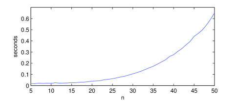
(a) Running time

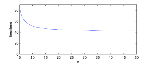
(b) Iterations

Figure 1: (a) Average running time until convergence of BP for $5\leq n\leq 50$. (b) Number of iterations.

4 Experiments

In this section we evaluate the performance of this algorithm in terms of running time and accuracy, and finally we exemplify a possible usage of the approximate permanent as a kernel function.

4.1 Running Time

We ran belief propagation to approximate the permanents of random matrices of sizes $n=[5,50]$, recording the total running time and the number of iterations to convergence. Surprisingly, the number of iterations to convergence initially decreased as $n$ grew, but appears to remain constant beyond $n>10$ or so. Running time still increased because the cost of updating each iteration well subsumes the decrease in iterations to convergence.

In our implementation, we checked for convergence by computing the absolute change in all the messages from the previous iteration, and considered the algorithm converged if the sum of all the changes of all $n^{3}$ messages was less than $1e-10$. In all cases, the resulting beliefs were consistent with each other within comparable precision to our convergence threshold. These experiments were run on a a 2.4 Ghz Intel Core 2 Duo Apple Macintosh running Mac OS X 10.5. The code is in $C$ and compiled using gcc version 4.0.1.

Table 1: Normalized Kendall distances between the rankings of random matrices based on their true permanents and the rankings based on approximate permanents. See Figure 2 for plots of the approximations.

n	Bethe	Sampling	Det.	Diag.
10	0.00023	0.0248	0.3340	0.0724
8	0.0028	0.1285	0.4995	0.4057
5	0.0115	0.0914	0.4941	0.3834

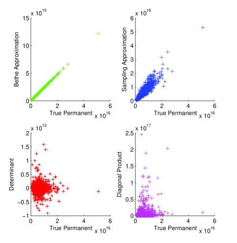
Figure 2: Plots of the approximated permanent versus the true permanent using four different methods. It is important to note that the scale of the y-axis varies from plot to plot. The diagonal is extremely erratic and the determinant underestimates so much that it is barely visible on the log scale. Sampling approximates values much closer in absolute distance to the true permanent but does not provide monotonicity in its approximations. Typically, this is more important than absolute accuracy. Here we illustrate the results from the $n=8$ case. We report results for $n=5$ and $10$ in Table 1.

4.2 Accuracy of Approximation

We evaluate the accuracy of our algorithm by creating 1000 random matrices of sizes 5, 8 and 200 matrices of size 10. The entries of each of these matrices were randomly drawn from a uniform distribution in the interval $[0,50]$. We computed the true permanents of these matrices, then computed approximate permanents using our Bethe approximation. We also computed an approximate using a naive sampling method, where we sample by choosing random permutations and storing a cumulative sum of each permutation’s corresponding product. We sampled for the same amount of actual time our belief propagation algorithm took to converge. Finally we also computed two weak approximations: the determinant and the scaled product of the diagonal entries.

In order to be able to compare to the true permanent, we had to limit this analysis to small matrices. However, since MCMC sampling methods such as in [10] take ${\cal O}(n^{10})$ time to reach less than some $\epsilon$ error, as matrix size increases, the precision achievable in comparable time to our algorithm would decrease. We scale the cumulative sum by $\frac{n!}{s}$, where $s$ is the number of samples. This is the ratio of the total possible permutations and the number of samples.

In our experiments, determinants and the products of diagonals are neither accurate nor consistent approximations of the permanent. Sampling, however, is accurate with respect to absolute distance to the permanent, so for applications where that is most important, it may be best to apply some sort of sampling method. Our Bethe approximation seems the most consistent. While the approximations of the permanent are off by a large amount, they seem to be consistently off by some monotonic function of the true permanent. In many cases, this virtue is more important than the absolute accuracy, since most applications requiring a matrix permanent likely compare the permanents of various matrices. These results are visualized for $n=8$ in Figure 2.

To measure the monotonicity and consistency of these approximations, we consider the Kendall distance [5] between the ranking of the random matrices according to the true permanent and their rankings according to the approximations. Kendall distance is a popular way of measuring the distance between two permutations. The Kendall distance between two permutations $\pi_{1}$ and $\pi_{2}$ is

$$D_{\textrm{Kendall}}(\pi_{1},\pi_{2}) = \sum_{i=1}^{n}\sum_{j=i+1}^{n}I\left((\pi_{1}(i)<\pi_{1}(j))\wedge(\pi_{2}(i)>\pi_{2}(j))\right).$$

In other words, it is the total number of pairs where $\pi_{1}$ and $\pi_{2}$ disagree on the ordering. We normalize the Kendall distance by dividing by $\frac{n(n-1)}{2}$, the maximum possible distance between permutations, so the distance will always be in the range $[0,1]$. Table 1 lists the Kendall distances between the true permanent ranking and the four approximations. The Kendall distance of the Bethe approximation is consistently less than that of our sampler.

Table 2: Left: Error rates of running SVM using various kernels on the original three UCI datasets and data where the features are shuffled randomly for each datum. Right: UCI resampled pendigits data with order of points removed. Error rates of 1-versus-all multi-class SVM using various kernels.

Kernel	Heart	Pima	Ion.
Original Linear	0.1600	0.2600	0.1640
Orig. RBF $\sigma=0.3$	0.2908	0.3160	0.1240
Orig. RBF $\sigma=0.5$	0.2158	0.3220	0.0760
Orig. RBF $\sigma=0.7$	0.1912	0.2760	0.0960
Shuffled Linear	0.2456	0.3080	0.2640
Shuff. RBF $\sigma=0.3$	0.4742	0.3620	0.4840
Shuff. RBF $\sigma=0.5$	0.3294	0.3140	0.3580
Shuff. RBF $\sigma=0.7$	0.2964	0.3280	0.2700
Bethe $\sigma=0.3$	0.2192	0.2900	0.1000
Bethe $\sigma=0.5$	0.2140	0.2900	0.1380
Bethe $\sigma=0.7$	0.2164	0.2920	0.1380

Kernel	PenDigits
Sorted Linear	0.3960
Sorted RBF $\sigma=0.2$	0.4223
Sorted RBF $\sigma=0.3$	0.3407
Sorted RBF $\sigma=0.5$	0.3277
Shuffled Linear	0.7987
Shuff. RBF $\sigma=0.2$	0.9183
Shuff. RBF $\sigma=0.3$	0.9120
Shuff. RBF $\sigma=0.5$	0.8657
Bethe $\sigma=0.2$	0.1463
Bethe $\sigma=0.3$	0.1190
Bethe $\sigma=0.5$	0.1707

4.3 Approximate Permanent Kernel

To illustrate a possible usage of an efficient permanent approximation, we use a recent result [2] proving that the permanent of a valid kernel matrix between two sets of points is also a valid kernel between point sets. Since the permanent is invariant to permutation, we decided to try a few classification tasks using an approximate permanent kernel. The permanent kernel is computed by first computing a valid subkernel between a pairs of elements in two sets, then the permanent of those subkernel evaluations is taken as the kernel value between the data. Surprisingly, in experiments the kernel matrix produced by our algorithm was a valid positive definite matrix. This discovery opens up some intriguing questions to be explored later.

We ran a similar experiment to [15] where we took a the first 200 examples of each of the Cleveland Heart Disease, Pima Diabetes, and Ionosphere datasets from the UCI repository [4], and randomly permuted the features of each example, then compare the result of training an SVM on this shuffled data. We also provide the performance of the kernels on the unshuffled data for comparison. After normalizing the features of the data to the $[0,1]^{D}$ box, we chose three reasonable settings of $\sigma$ for the RBF kernels and cross validated over various settings of the regularization parameter $C$. We used RBF kernels between pairs of data as the permanent subkernel. Finally, we report the average error over 50 random splits of 150 training points and 50 testing points. Not surprisingly, the permanent kernel is robust to the shuffling and outperforms the standard kernels.

We also tested the Bethe kernel on the pendigits dataset, also from the UCI repository. The original pendigits data consists of stylus coordinates of test subjects writing digits. We used the preprocessed version that has been resampled spatially and temporally. However, we omit the order information and treat the input as a cloud of unordered points. Since there is a natural spatial interpretation of this data, so we compare to sorting by distance from origin, a simple method of handling unordered data. We chose slightly different $\sigma$ values for the RBF kernels. For this dataset, there are 10 classes, one for each digit, so we used a one-versus-all strategy for multi-class classification. Here we averaged over only 10 random splits of 300 training points and 300 testing points (see Table 2).

Based on our experiments, the permanent kernel typically does not outperform standard kernels when permutation invariance is not inherently necessary in the data, but when we induce the necessity of such invariance, its utility becomes clear.

5 Discussion and Future Directions

We have described an algorithm based on BP over a specific distribution that allows an efficient approximation of the $\#P$ matrix permanent operation. We write a probability distribution over matchings and use Bethe free energy to approximate the partition function of this distribution. The algorithm is significantly faster than sampling methods, but attempts to minimize a function that approximates the permanent. Therefore it is limited by the quality of the Bethe approximation so it cannot be run longer to obtain a better approximation like sampling methods can. However, we have shown that even on small matrices where sampling methods can achieve extremely high accuracy of approximation, our method is more well behaved than sampling, which can approach the exact value from above or below.

In the future, we can try other methods of approximating the partition function such as generalized belief propagation [18], which takes advantage of higher order Kikuchi approximations of free energy. Unfortunately the structure of our graphical model causes higher order interactions to become expensive quickly, since each variable has exactly $N$ neighbors. Similarly, the bounds on the partition function in [17] are based on spanning subtrees in the graph, and again the fully connected bipartite structure makes it difficult to capture the true behavior of the distribution with trees.

Finally, the positive definiteness of the kernels we computed is surprising, and requires further analysis. The exact permanent of a valid kernel forms a valid Mercer kernel [2] because it is a sum of positive products, but since our algorithm outputs the results of an iterative approximation of the permanent, it is not obvious why the resulting output would obey the positive definite constraints.

Acknowledgments

References

- [1] M. Bayati, D. Shah, and M. Sharma. Maximum weight matching via max-product belief propagation. In Proc. of the IEEE International Symposium on Information Theory, 2005.
- [2] M. Cuturi. Permanents, transportation polytopes and positive definite kernels on histograms. In International Joint Conference on Artificial Intelligence, IJCAI, 2007.
- [3] P. Dagum and M. Luby. Approximating the permanent of graphs with large factors. Theoretical Computer Science, 102(2):283–305, 1992.
- [4] C.L. Blake D.J. Newman, S. Hettich and C.J. Merz. UCI repository of machine learning databases, 1998.
- [5] R. Fagin, R. Kumar, and D. Sivakumar. Comparing top k lists, 2003.
- [6] T. Heskes. Stable fixed points of loopy belief propagation are local minima of the bethe free energy. In S. Thrun S. Becker and K. Obermayer, editors, Advances in Neural Information Processing Systems 15, pages 343–350. MIT Press, Cambridge, MA, 2003.
- [7] T. Heskes. Convexity arguments for efficient minimization of the bethe and kikuchi free energies. Journal of Artificial Intelligence Research, 26, 2006.
- [8] Tom Heskes. On the uniqueness of loopy belief propagation fixed points. Neural Comput., 16(11):2379–2413, 2004.
- [9] B. Huang and T. Jebara. Loopy belief propagation for bipartite maximum weight b-matching. In Artificial Intelligence and Statistics (AISTATS), 2007.
- [10] M. Jerrum, A. Sinclair, and E. Vigoda. A polynomial-time approximation algorithm for the permanent of a matrix with nonnegative entries. J. ACM, 51(4):671–697, 2004.
- [11] Knopp and Sinkhorn. Concerning nonnegative matrices and doubly stochastic matrices. Pacific Journal of Mathematics, 1967.
- [12] Anand Rangarajan, Alan Yuille, and Eric Mjolsness. Convergence properties of the softassign quadratic assignment algorithm. Neural Comput., 11(6):1455–1474, 1999.
- [13] H. J. Ryser. Combinatorial mathematics. The Carus Mathematical Monographs, (14), 1963.
- [14] R. A. Servedio and A. Wan. Computing sparse permanents faster. Inf. Process. Lett., 96(3):89–92, 2005.
- [15] P. Shivaswamy and T. Jebara. Permutation invariant svms. In International Conference on Machine Learning, ICML, 2006.
- [16] S. Tatikonda and M. Jordan. Loopy belief propagation and Gibbs measures. In Proc. Uncertainty in Artificial Intell., vol. 18, 2002.
- [17] M. Wainwright, T. Jaakkola, and A. Willsky. A new class of upper bounds on the log partition function, 2002.
- [18] J.S. Yedidia, W.T. Freeman, and Y. Weiss. Constructing free-energy approximations and generalized belief propagation algorithms. IEEE Transactions on Information Theory, 51(7), 2005.
- [19] A. L. Yuille. Cccp algorithms to minimize the bethe and kikuchi free energies: Convergent alternatives to belief propagation. Neural Computation, 14(7):1691–1722, 2002.