Power-enhanced multiple decision functions controlling family-wise error and false discovery rates

Abstract

Improved procedures, in terms of smaller missed discovery rates (MDR), for performing multiple hypotheses testing with weak and strong control of the family-wise error rate (FWER) or the false discovery rate (FDR) are developed and studied. The improvement over existing procedures such as the Šidák procedure for FWER control and the Benjamini–Hochberg (BH) procedure for FDR control is achieved by exploiting possible differences in the powers of the individual tests. Results signal the need to take into account the powers of the individual tests and to have multiple hypotheses decision functions which are not limited to simply using the individual $p$-values, as is the case, for example, with the Šidák, Bonferroni, or BH procedures. They also enhance understanding of the role of the powers of individual tests, or more precisely the receiver operating characteristic (ROC) functions of decision processes, in the search for better multiple hypotheses testing procedures. A decision-theoretic framework is utilized, and through auxiliary randomizers the procedures could be used with discrete or mixed-type data or with rank-based nonparametric tests. This is in contrast to existing $p$-value based procedures whose theoretical validity is contingent on each of these $p$-value statistics being stochastically equal to or greater than a standard uniform variable under the null hypothesis. Proposed procedures are relevant in the analysis of high-dimensional “large $M$, small $n$” data sets arising in the natural, physical, medical, economic and social sciences, whose generation and creation is accelerated by advances in high-throughput technology, notably, but not limited to, microarray technology.

, and

t1Supported by NSF Grant DMS-08-05809, NIH Grant RR17698 and EPA Grant RD-83241902-0 to University of Arizona with subaward number Y481344 to the University of South Carolina.

1 Introduction and motivation

The advent of modern technology, epitomized by the microarray, has led to the generation of very high-dimensional data pertaining to characteristics of a large number, $M$, of attributes, hereon called genes, associated with usually a small number, $n$, of units or subjects. Several such data sets are, for example, described in Efr08 , and these are the inputs to so-called parallel inference problems. The most common form of inference is multiple hypotheses testing, wherein for the $m$th gene there are two competing hypotheses, a null hypothesis $H_{m0}$ and an alternative hypothesis $H_{m1}$, for which a decision is to be made based on the data. In such multiple decision-making, there is a need to be cognizant and cautious of the Hyde-ian nature of multiplicity, while also exploiting the Jekyll-ian potentials of multiplicity Stevenson03 . Furthermore, this entails a tenuous balance between two competing desires: controlling the rate of rejection of correct null hypotheses, while at the same time maintaining the rate of discovery of correct alternative hypotheses.

As in single-pair hypothesis testing, a type I error occurs when a correct null hypothesis is rejected, while a type II error occurs when a false null hypothesis is not rejected. Several type I errors have been proposed in multiple testing; see DudShaBol03 and DudLaa08 . Our focus is on the weak family wise error rate (FWER), the probability of rejecting at least one null hypothesis when all the nulls are correct; strong FWER, the probability of rejecting at least one correct null hypothesis; and false discovery rate (FDR), the expected proportion of the number of false rejections of nulls relative to the number of rejections Sor89 , BenHoc95 . Our type II error rate is the missed discovery rate (MDR), the expected number of false nonrejections of null hypotheses. Other type II errors have been discussed in DudShaBol03 , Sto03 , DudGilVan07 , Efr07 , DudLaa08 . The usual framework in developing multiple decision functions is to bound the chosen type I error rate, and then minimize or make small the MDR. For example, a procedure controlling weak FWER, under an independence assumption, is that of Šidák Sid67 ; while a conservative one not requiring independence is the Bonferroni procedure Bon37 . For FDR control, the most common procedure is the BH procedure BenHoc95 . Control of type I error measures related to the FDR have also been discussed in EfrTibStoTus01 , GenWas02 , Sto02 , Sto03 , Efr04 , Efr07 , SunCai07 , Efr08 , while SchSpj82 , LanLinFer05 , JinCai07 focused on estimation of the proportion of correct null hypotheses.

Procedures like the Šidák, Bonferroni and BH, rely on the set of $p$-values of individual tests. Their validity hinges on each $p$-value statistic being stochastically equal to or greater than a standard uniform variable under the null hypothesis. This fails, however, with noncontinuous variables or when rank-based nonparametric tests are used. Crucially, $p$-value based procedures also do not exploit the power characteristics of the individual tests, contrary to Neyman and Pearson’s NeyPea33 adage that such considerations are germane in constructing optimal tests. Such $p$-value based procedures are fine in exchangeable settings where power characteristics of the individual tests are identical, but not in situations where genes or subclasses of genes have different structures; see EfrAAS08 , FerFriRueThoKon08 , RoqWie09 .

Some papers dealing with procedures exploiting the power functions are Spj72 , WesKriYou98 . The use of weighted $p$-values to improve type II performance have also been explored in GenRoeWas06 , WasRoe06 , RubDudLaa06 , KanYeLiuAllGao09 , RoqWie09 . Other approaches for optimal procedures are those in Sto07 , StoDaiLee07 which employ a Neyman–Pearson approach and SunCai07 where oracle and adaptive compound rules were obtained. Compound rules are characterized by information borrowing from each of the genes, so a decision function for a specific gene utilizes information from other genes. Decision-theoretic and Bayesian approaches were also implemented in MulParRobRou04 , SarZhoGho08 , ScoBer06 , Efr08 , GuiMulZha09 . More recently, EfrAAS08 argues for separate subclass analysis, while FerFriRueThoKon08 proposed use of external covariates, with the procedures having a Bayes and empirical Bayes flavor.

The main goal of this paper is to develop better multiple testing procedures controlling weak FWER, strong FWER and FDR by taking into account the individual powers of the tests. We focus on the most fundamental setting where the null and alternative hypotheses for each gene are both simple. This is also the setting in RoqWie09 . This admits, as starting point, the Neyman–Pearson most powerful (MP) test for each pair of hypotheses. Each MP test will have a power, but we will see that it is beneficial to look at each of these powers as function of their MP test’s size, their so-called receiver operating characteristic (ROC) function.

The paper proceeds as follows. Section 2 presents the decision-theoretic elements. Section 3 reviews and reexamines MP tests, $p$-value statistics and ROC functions. Section 4 develops the optimal weak FWER-controlling procedure, with existence and uniqueness established in Section 4.2. Section 4.3 analytically describes the procedure for differentiable ROC functions. Section 4.4 provides a concrete example using normal distributions, while Section 4.5 discusses a size-investing strategy for optimality. Section 5 discusses limitations, extensions and connections: Section 5.1 deals with the restriction to the class of simple procedures; Section 5.2 deals with extensions to the composite hypotheses setting in the presence of the monotone likelihood ratio (MLR) property; and Section 5.3 relates the optimal procedure to weighted $p$-value based procedures. Section 6 develops an improved procedure which strongly controls the FWER, whereas Section 7 develops an improved procedure which controls FDR. The development of these new procedures is anchored on the weak FWER-controlling optimal procedure. We establish that the sequential Šidák and BH procedures are special cases of these more general procedures. Section 8 provides a modest simulation study demonstrating that the new FDR-controlling procedure improves on the BH procedure. Section 9 contains a summary and some concluding remarks.

To manage the length of the paper and provide more focus on the main ideas and results, technical proofs of lemmas, propositions, theorems and corollaries are all gathered in the supplemental article PenHabWu10Supp .

2 Mathematical setting

Let $(\Omega,\mathcal{F},\mathbf{P})$ be a probability space and $\mathcal{M}=\{1,2,\ldots,M\}$ an index set with $M$ a known positive integer. For each $m\in\mathcal{M}$, let $X_{m}\dvtx(\Omega,\mathcal{F})\rightarrow(\mathcal{X}_{m},\mathcal{B}_{m})$, $\mathcal{X}_{m}$ some space with $\sigma$-field of subsets $\mathcal{B}_{m}$. Form the product space $(\mathcal{X},\mathcal{B})$ with $\mathcal{X}=\times_{m\in\mathcal{M}}\mathcal{X}_{m}$ and $\mathcal{B}=\sigma(\times_{m\in\mathcal{M}}\mathcal{B}_{m})$ so $X=(X_{1},X_{2},\ldots,X_{M})\dvtx(\Omega,\mathcal{F})\rightarrow(\mathcal{X},\mathcal{B})$. The probability measure of $X$ is $Q=\mathbf{P}X^{-1}$, while the (marginal) probability measure of $X_{m}$ is $Q_{m}=PX_{m}^{-1}$. For each $m\in\mathcal{M}$, let $Q_{m0}$ and $Q_{m1}$ be two known probability measures on $(\mathcal{X}_{m},\mathcal{B}_{m})$. We assume that $Q\in\mathcal{Q}$, a class of probability measures on $(\mathcal{X},\mathcal{B})$ with marginal probability measure $Q_{m}\in\{Q_{m0},Q_{m1}\}$ for each $m\in\mathcal{M}$. Let $\theta=(\theta_{1},\ldots,\theta_{M})\dvtx\mathcal{Q}\rightarrow\Theta\equiv\{0,1\}^{M}$ with $\theta_{m}(Q)=I\{Q_{m}=Q_{m1}\}$, $I\{\cdot\}$ denoting indicator function. Define, for each $Q\in\mathcal{Q}$, the subcollections $\mathcal{M}_{0}\equiv\mathcal{M}_{0}(Q)=\{m\in\mathcal{M}\dvtx\theta_{m}(Q)=0\}$ and $\mathcal{M}_{1}\equiv\mathcal{M}_{1}(Q)=\{m\in\mathcal{M}\dvtx\theta_{m}(Q)=1\}$. In this paper, we shall impose an independence condition given by:

Condition (I).

$(X_{m},m\in\mathcal{M}_{0}(Q))$ is an independent collection of random entities, that is, $\forall B_{m}\in\mathcal{B}_{m}$, $Q(\times_{m\in\mathcal{M}_{0}(Q)}B_{m})=\prod_{m\in\mathcal{M}_{0}(Q)}Q_{m}(B_{m})$.

However, the collection $(X_{m},m\in\mathcal{M}_{1}(Q))$ need not be an independent collection, but it is independent of $(X_{m},m\in\mathcal{M}_{0}(Q))$. Two extreme subcollections of $\mathcal{Q}$ are $\mathcal{Q}_{0}=\{Q\in\mathcal{Q}\dvtx\theta_{m}(Q)=0,\forall m\in\mathcal{M}\}$ and $\mathcal{Q}_{1}=\{Q\in\mathcal{Q}\dvtx\theta_{m}(Q)=1,\forall m\in\mathcal{M}\}$. By Condition (I), $\mathcal{Q}_{0}$ is a singleton set, $Q_{0}$ will denote its element; while $\mathcal{Q}_{1}$ need not be a singleton set. The decision problem is to determine $\mathcal{M}_{0}(Q)$ and $\mathcal{M}_{1}(Q)$ based on $X$, which is equivalent to simultaneously testing the $M$ pairs of hypotheses $H_{m0}\dvtx Q_{m}=Q_{m0}$ versus $H_{m1}\dvtx Q_{m}=Q_{m1}$ for $m\in\mathcal{M}$.

We adopt a decision-theoretic framework similar to SarZhoGho08 . The action space is $\mathcal{A}=\{0,1\}^{M}$ with generic element $a=(a_{1},a_{2},\ldots,a_{M})^{t}\in\mathcal{A}$ with $a_{m}=0(1)$ meaning $H_{m0}$ is accepted (rejected). The parameter space is $\mathcal{Q}$, though the effective parameter space is $\Theta=\{0,1\}^{M}$ with generic element $\theta=(\theta_{1},\theta_{2},\ldots,\break\theta_{M})^{t}$. We introduce several loss functions, $L\dvtx\mathcal{A}\times\mathcal{Q}\rightarrow\Re_{+}$, defined via

$$L_{0}(a,Q) = I\bigl{\{}a^{t}\bigl{(}1-\theta(Q)\bigr{)}\geq 1\bigr{\}};$$ (1)

$$L_{1}(a,Q) = \biggl{[}\frac{a^{t}(1-\theta(Q))}{a^{t}1}\biggr{]}I\{a^{t}1>0\};$$ (2)

$$L_{2}(a,Q) = {(1-a)^{t}\theta(Q)},$$ (3)

with the convention that $0/0=0$ and $1$ is an $M\times 1$ vector of $1$’s. The loss function $L_{0}(a,Q)$ equals 1 if and only if at least one false discovery is committed. The loss $L_{1}(a,Q)$ is the false discovery proportion, being the ratio between the number of false discoveries and the number of discoveries; whereas the loss $L_{2}(a,Q)$ is the number of missed discoveries being the number of true alternative hypotheses that were not discovered. We focus on this missed discovery number since the relevant question is how many correct alternatives [$\theta(Q)^{t}1$] were missed by using the action $a$? See also RoqWie09 which essentially uses this loss function to induce their power metric. Other types of losses, such as the false negative proportion with $(a,Q)\mapsto{[(1-a)^{t}\theta(Q)]}/{[(1-a)^{t}1]}I\{(1-a)^{t}1>0\}$, have also been considered; see GenWas02 , SarZhoGho08 .

A nonrandomized multiple decision function (MDF) is a $\delta\dvtx(\mathcal{X},\mathcal{B})\rightarrow(\mathcal{A}$, $\sigma(\mathcal{A}))$, where $\sigma(\mathcal{A})$ is the power set of $\mathcal{A}$. Such an MDF may be represented by $\delta(x)=(\delta_{1}(x),\delta_{2}(x),\ldots,\delta_{M}(x))^{t}$, where $\delta_{m}(x)\in\{0,1\}$. In general, each $\delta_{m}$ could be made to depend on the full data $x$ instead of just $x_{m}$. We denote by $\mathcal{D}$ the class of all nonrandomized MDFs. A randomized MDF may also be considered. Denote by $\mathcal{P}(\mathcal{A})$ the space of all probability measures over $(\mathcal{A},\sigma(\mathcal{A}))$. A randomized MDF is a $\delta^{*}\dvtx(\mathcal{X},\mathcal{B})\rightarrow(\mathcal{P}(\mathcal{A}),\sigma(\mathcal{P}(\mathcal{A})))$. For a realization $X=x$, an action is chosen from $\mathcal{A}$ according to the probability measure $\delta^{*}(x)$. Denote by $\mathcal{D}^{*}$ the space of all randomized MDFs. Clearly, $\mathcal{D}\subset\mathcal{D}^{*}$. By augmenting data $X$ with a randomizer $U\sim U(0,1)$ which is independent of $X$, randomized MDFs could be made nonrandomized with respect to the augmented data $(X,U)$. Henceforth, $\mathcal{D}$ represents all nonrandomized MDFs $\delta(X,U)$’s based on $(X,U)$.

For brevity of notation, $\mathbf{P}_{Q}\{f(X,U)\in B\}$ and $E_{Q}\{f(X,U)\}$ represent probability and expectation with respect to $(X,U)$ with $X\sim Q$, $U\sim U(0,1)$ and $X$ and $U$ independent. For $\delta\in\mathcal{D}$ and the loss functions defined earlier, we have the risk functions

$$R_{0}(\delta,Q) = E_{Q}\{L_{0}(\delta(X,U),Q)\};$$ (4)

$$R_{1}(\delta,Q) = E_{Q}\{L_{1}(\delta(X,U),Q)\};$$ (5)

$$R_{2}(\delta,Q) = E_{Q}\{L_{2}(\delta(X,U),Q)\}.$$ (6)

Given a $\delta=(\delta_{1},\delta_{2},\ldots,\delta_{M})^{t}$, let $\pi_{\delta}(Q)=(\pi_{\delta_{1}}(Q),\pi_{\delta_{2}}(Q),\ldots,\pi_{\delta_{M}}(Q))^{t}$ with $\pi_{\delta_{m}}(Q)=E_{Q}\{\delta_{m}(X,U)\}$ be its vector of power functions. Then (6) becomes $R_{2}(\delta,Q)=(1-\pi_{\delta}(Q))^{t}\theta(Q)$. In terms of these risk functions, for $\delta\in\mathcal{D}$, its weak FWER is $\operatorname{FWER}(\delta)=R_{0}(\delta,Q_{0})$. If each $\delta_{m}$ depends only on $X_{m}$ and $U$, by Condition (I),

$$\operatorname{FWER}(\delta)=1-E\biggl{\{}\prod_{m\in\mathcal{M}}[1-\mathbf{P}_{Q_{m0}}\{\delta_{m}(X_{m},U)=1|U\}]\biggr{\}},$$ (7)

where the expectation is with respect to $U$. When $Q=Q_{0}$ and with the $m$th component $\delta_{m}^{*}$ of the randomized MDF depending only on $X_{m}$, an alternative formulation is to have $U=(U_{1},U_{2},\ldots,U_{M})$ a vector of i.i.d. $U(0,1)$ variables which is independent of the $X_{m}$’s. The $m$th component may then be redefined via $\delta_{m}(X_{m},U_{m})=I\{U_{m}\leq\delta_{m}^{*}(X_{m})\}$. Then (7) becomes $\operatorname{FWER}(\delta)=1-\prod_{m\in\mathcal{M}}[1-\mathbf{P}_{Q_{m0}}\{\delta_{m}(X_{m},U_{m})=1\}]$.

The risk function $R_{1}(\delta,Q)$ is the false discovery rate (FDR) of $\delta$ at $Q$ BenHoc95 ; while the risk function $R_{2}(\delta,Q)$ will be called the missed discovery rate (MDR) of $\delta$ at $Q$. The adjective “rate” is somewhat misleading since $R_{2}(\delta,Q)$ takes values in $[0,|\mathcal{M}_{1}(Q)|]$ instead of $[0,1]$; however, this does not cause difficulty since, given the true underlying probability measure $Q$ of $X$, $|\mathcal{M}_{1}(Q)|$ is constant. This risk is related to the expected number of true positives (ETP), an error measure used in Spj72 , Sto07 , via $\operatorname{ETP}(\delta,Q)=|\mathcal{M}_{1}(Q)|-R_{2}(\delta,Q)$.

To find an optimal MDF weakly controlling FWER in a subclass $\mathcal{D}_{0}\subseteq\mathcal{D}$, a threshold $\alpha\in(0,1)$ is specified and then we seek a $\delta^{*}\in\mathcal{D}_{0}$ with $R_{0}(\delta^{*},Q_{0})=\operatorname{FWER}(\delta^{*})\leq\alpha$, and such that for any $\delta\in\mathcal{D}_{0}$ satisfying $R_{0}(\delta,Q_{0})=\break\operatorname{FWER}(\delta)\leq\alpha$, we have $\sup_{Q\in\mathcal{Q}}R_{2}(\delta^{*},Q)\leq\sup_{Q\in\mathcal{Q}}R_{2}(\delta,Q)$. This criterion has a minimax flavor. One may require only that $R_{2}(\delta^{*},Q^{*})\leq R_{2}(\delta,Q^{*})$ where $Q^{*}$ is the true, but unknown, probability law of $X$; but this may be too strong to preclude a solution to the optimization problem. However, see Sto07 for a situation with a different type I error and where an optimal, albeit an oracle, solution for minimizing $R_{2}(\delta,Q^{*})$ is possible. Observe that for $\delta\in\mathcal{D}$, by using the representation of $R_{2}(\delta,Q)$ in terms of the powers, $\sup_{Q\in\mathcal{Q}}R_{2}(\delta,Q)=\sup_{Q\in\mathcal{Q}_{1}}R_{2}(\delta,Q)=M-\inf_{Q\in\mathcal{Q}_{1}}\sum_{m\in\mathcal{M}}\pi_{\delta_{m}}(Q)$. The optimality condition on the MDR amounts therefore to maximizing $\sum_{m\in\mathcal{M}}\pi_{\delta_{m}}(Q_{m1})$. Interestingly, if we had standardized the loss function $L_{2}(a,Q)$ to take values in $[0,1]$ via division by $|\mathcal{M}_{1}(Q)|=\theta(Q)^{t}1$, the minimax justification does not carry through!

For strong FWER control, we seek a compound MDF, $\delta^{*}\in\mathcal{D}$, with $R_{0}(\delta^{*}$, $Q^{*})\leq\alpha$ whatever the true, but unknown, probability law $Q^{*}$ of $X$ is, and with $\sum_{m\in\mathcal{M}}\pi_{\delta_{m}^{*}}(Q_{m1})$ large, possibly maximal, among all $\delta\in\mathcal{D}$ satisfying $R_{0}(\delta,Q^{*})\leq\alpha$. For (strong) FDR-control, a threshold $q^{*}\in(0,1)$ is specified and we seek a compound MDF, $\delta^{*}\in\mathcal{D}$, such that, whatever $Q^{*}$ is, $R_{1}(\delta^{*},Q^{*})\leq q^{*}$, and with $\sum_{m\in\mathcal{M}}\pi_{\delta_{m}^{*}}(Q_{m1})$ large, possibly maximal, among all $\delta\in\mathcal{D}$ satisfying $R_{1}(\delta,Q^{*})\leq q^{*}$. For discussion of weak and strong control, refer to DudShaBol03 , DudLaa08 . Discussion of optimality in multiple testing can be found in LehRomSha05 where maximin optimality results are established for some step-down and step-up MTPs.

3 Revisiting MP tests and $p$-value statistics

An MDF $\delta\in\mathcal{D}$ whose $m$th component $\delta_{m}$ depends only on $(X_{m},U_{m})$ for every $m\in\mathcal{M}$ is called simple; otherwise, it is compound. The subclass of simple MDFs, denoted by $\mathcal{D}_{0}$, will be our initial focus in searching for an optimal weak FWER-controlling MDF. The resulting optimal MDF will then anchor our search for strong FWER- and FDR-controlling compound MDFs. Before implementing this program, we introduce the unifying concept of decision processes.

3.1 Decision processes, ROC functions, $p$-value statistics

First, a brief review. Let $X\dvtx(\Omega,\mathcal{A})\rightarrow(\mathcal{X},\mathcal{B})$ and $Q=\mathbf{P}X^{-1}$. Based on $X$, consider testing the pair of hypotheses $H_{0}\dvtx Q=Q_{0}$ versus $H_{1}\dvtx Q=Q_{1}$, where $Q_{0}$ and $Q_{1}$ are two probability measures on $(\mathcal{X},\mathcal{B})$. Let $q_{0}$ and $q_{1}$ be versions of the densities of $Q_{0}$ and $Q_{1}$ with respect to some fixed dominating measure $\nu$, for example, $\nu=Q_{0}+Q_{1}$. Recall that a test or decision function is a $\delta\dvtx(\mathcal{X},\mathcal{B})\rightarrow([0,1],\sigma[0,1])$, with $\sigma[0,1]$ the Borel sigma-field on $[0,1]$. Given $X=x$, $\delta(x)$ is the probability of deciding in favor of $H_{1}$. Its size is $\alpha_{\delta}=E_{Q_{0}}\delta(X);$ it is of level $\alpha\in[0,1]$ if $\alpha_{\delta}\leq\alpha$. Its power is $\pi_{\delta}=E_{Q_{1}}\delta(X)$. $\delta^{*}$ is most powerful (MP) of level $\alpha$ if $\alpha_{\delta^{*}}\leq\alpha$ and for all $\delta$ with $\alpha_{\delta}\leq\alpha$, we have $\pi_{\delta^{*}}\geq\pi_{\delta}$.

Definition 3.1.

A collection $\Delta=\{\delta_{\eta}\dvtx\eta\in[0,1]\}$ of test functions such that, a.e. $[Q]$, $\delta_{0}(x)=0$, $\delta_{1}(x)=1$ and $\eta\mapsto\delta_{\eta}(x)$ is nondecreasing and right-continuous, is a decision process. Its size function is $A_{\Delta}\dvtx[0,1]\rightarrow[0,1]$ and its power function is $\rho_{\Delta}\dvtx[0,1]\rightarrow[0,1]$, where $A_{\Delta}(\eta)=\alpha_{\delta_{\eta}}=E_{Q_{0}}\delta_{\eta}(X)$ and $\rho_{\Delta}(\eta)=\pi_{\delta_{\eta}}=E_{Q_{1}}\delta_{\eta}(X)$. Its receiver operating characteristic (ROC) curve is $\operatorname{ROC}(\Delta)\equiv\operatorname{Graph}\{(A_{\Delta}(\eta),\rho_{\Delta}(\eta))\dvtx\eta\in[0,1]\}$. If $A_{\Delta}(\eta)=\eta$ for all $\eta\in[0,1]$, $\eta\mapsto\rho_{\Delta}(\eta)$ is the ROC function of $\Delta$.

The use of the phrase power function in Definition 3.1 is atypical since we are not viewing this as a function of a parameter as is the usual meaning of this phrase. However, for lack of a better name, we shall adopt this terminology. In the sequel, $\delta_{\eta}$ and $\delta(\eta)$ will be used interchangeably to also represent $\delta(\cdot;\eta)$.

Let $L\dvtx(\mathcal{X},\mathcal{B})\rightarrow(\Re_{+},\sigma(\Re_{+}))$ be a version of the likelihood ratio function: $L(x)=q_{1}(x)/q_{0}(x)$ a.e. $[\nu]$. Let $G_{0}(\cdot)$ and $G_{1}(\cdot)$ be the distribution functions of $L(X)$ when $\mathcal{L}(X)=Q_{0}$ and $\mathcal{L}(X)=Q_{1}$, where $\mathcal{L}(X)$ is probability measure of $X$. For a monotone nondecreasing right-continuous function $M(\cdot)$ from $\Re$ into $\Re$, let $M^{-1}(r)=\inf\{x\in\Re\dvtx M(x)\geq r\}$ and $\Delta M(r)=M(r)-M(r-)$. By the Neyman–Pearson fundamental lemma NeyPea33 , the MP test function of level $\eta$ for testing $H_{0}$ versus $H_{1}$ is

$$\delta^{*}(X;\eta)\equiv\delta^{*}_{\eta}=I\{L(X)>c(\eta)\}+\gamma(\eta)I\{L(X)=c(\eta)\},$$ (8)

where $c(\eta)=G_{0}^{-1}(1-\eta)$ and $\gamma(\eta)={(G_{0}(c(\eta))-(1-\eta))}/{\Delta G_{0}(c(\eta))}$. Let $U\sim U(0,1)$ be independent of $X$. Redefine $\delta^{*}$ via $\delta_{\eta}^{**}\equiv\delta^{**}(X,U;\eta)=I\{U\leq\delta^{*}(X;\eta)\}$, which is nonrandomized w.r.t. $(X,U)$. In essence, with the aid of an auxiliary randomizer $U$, the MP test could always be made nonrandomized. The decision process formed from these MP tests, given by

$$\Delta^{*}=\{\delta_{\eta}^{*}\dvtx\eta\in[0,1]\}=\{\delta_{\eta}^{**}\dvtx\eta\in[0,1]\},$$ (9)

is called the most powerful (MP) decision process. The power (at $Q=Q_{1}$) of the MP test $\delta_{\eta}^{*}$ or $\delta_{\eta}^{**}$ is

$$\rho_{\Delta^{*}}(\eta)\equiv\pi_{\delta^{*}_{\eta}}=\pi_{\delta^{**}_{\eta}}=1-G_{1}(c(\eta))+\gamma(\eta)\Delta G_{1}(c(\eta)).$$ (10)

It is well known Leh97 that $\pi_{\delta^{*}_{\eta}}<1$ implies $\alpha_{\delta^{*}_{\eta}}=\eta$. We denote by $A_{\Delta^{*}}$ and $\rho_{\Delta^{*}}$ the size and power functions of $\Delta^{*}$. If $\pi_{\delta^{*}_{\eta}}<1$ for all $\eta<1$, then $\eta\mapsto\rho_{\Delta^{*}}(\eta)$ is the ROC function of $\Delta^{*}$. We present below some important properties of this function.

Before stating the proposition, we reiterate that all formal proofs of propositions, theorems, lemmas and corollaries are in the supplemental article PenHabWu10Supp .

Proposition 3.1.

The function $\rho_{\Delta^{*}}\dvtx[0,1]\rightarrow[0,1]$ in (10) is concave, continuous and nondecreasing. Furthermore, $\rho_{\Delta^{*}}(\eta)\geq\eta$ and it is strictly increasing on the set $\mathcal{N}_{<}\equiv\{\eta\in[0,1]\dvtx\rho_{\Delta^{*}}(\eta)<1\}$.

Definition 3.2.

Let $\Delta=\{\delta_{\eta}\dvtx\eta\in[0,1]\}$ be a decision process, where $\delta_{\eta}\dvtx(\mathcal{X}\times[0,1],\mathcal{B}\otimes\sigma[0,1])\rightarrow(\{0,1\},\sigma\{0,1\})$. Its (randomized) $p$-value statistic is $S_{\Delta}\dvtx(\mathcal{X}\times[0,1],\mathcal{B}\otimes\sigma[0,1])\rightarrow([0,1],\sigma[0,1])$ with $S_{\Delta}(x,u)=\inf\{\eta\in[0,1]\dvtx\delta_{\eta}(x,u)=1\}$.

When $\forall(\eta,x,u)\dvtx\delta_{\eta}(x,u)=\delta_{\eta}(x)$, then $S_{\Delta}(X,U)$ is the usual $p$-value statistic. See also CoxHin74 for a more specialized definition of a randomized $p$-value statistic. We refer the reader to HabPen10 for properties of this $p$-value statistic and its use in existing FDR-controlling procedures.

Proposition 3.2.

Let $\Delta=\{\delta_{\eta}\dvtx\eta\in[0,1]\}$ be a decision process with $p$-value statistic $S_{\Delta}$. Then, for all $s\in[0,1]$, $H_{0}(s)\equiv\mathbf{P}_{Q_{0}}(S_{\Delta}\leq s)=A_{\Delta}(s)$ and $H_{1}(s)\equiv\mathbf{P}_{Q_{1}}(S_{\Delta}\leq s)=\pi_{\delta(s)}=\rho_{\Delta}(s)$. Consequently, $S_{\Delta}\sim U[0,1]$ under $\mathcal{L}(X)=Q_{0}$ if and only if $\forall\eta\in[0,1]\dvtx A_{\Delta}(\eta)=\eta$.

4 Optimal weak FWER control

Return now to the multiple decision problem in Section 2. We extend the notion of decision processes to the multiple decision setting.

Definition 4.1.

A collection $\bolds{\Delta}=(\Delta_{m}\dvtx m\in\mathcal{M})$, where $\Delta_{m}=(\delta_{m}(\eta)\dvtx\eta\in[0,1])$ is a decision process on $(\mathcal{X}\times[0,1]^{M},\mathcal{B}\otimes\sigma[0,1]^{M})$, is a multiple decision process (MDP). It is simple if each $\Delta_{m}$ is simple; otherwise, it is compound. When simple its multiple decision size function is $\mathbf{A}_{\bolds{\Delta}}=(A_{\Delta_{m}}\dvtx m\in\mathcal{M})$ and its multiple decision ROC function is $\bolds{\rho}_{\bolds{\Delta}}=(\rho_{\Delta_{m}}\dvtx m\in\mathcal{M})$, where $A_{\Delta_{m}}$ and $\rho_{\Delta_{m}}$ are the size and ROC functions of $\Delta_{m}$.

4.1 Optimization problem

Let $\bolds{\Delta}$ be a simple MDP. Then, a multiple decision size vector $\bolds{\eta}=(\eta_{m}\dvtx m\in\mathcal{M})\in\mathcal{N}\equiv[0,1]^{M}$ determines from $\bolds{\Delta}$ an MDF $\delta_{\bolds{\Delta}}(\bolds{\eta})=(\delta_{m}(\eta_{m})\dvtx m\in\mathcal{M})\in\mathcal{D}_{0}$. For this MDF, $\operatorname{FWER}(\delta_{\bolds{\Delta}}(\bolds{\eta}))=1-\prod_{m\in\mathcal{M}}[1-A_{\Delta_{m}}(\eta_{m})]$ and $R_{2}(\delta_{\bolds{\Delta}}(\bolds{\eta}),Q_{1})=M-\sum_{m\in\mathcal{M}}\rho_{\Delta_{m}}(\eta_{m})$ for $Q_{1}\in\mathcal{Q}_{1}$. Fix an FWER-threshold $\alpha\in(0,1)$. Suppose there exists a multiple decision size vector $\bolds{\eta}_{\bolds{\Delta}}^{*}(\alpha)\in\mathcal{N}$ such that

$$\bolds{\eta}_{\bolds{\Delta}}^{*}(\alpha)=\mathop{\arg\max}_{\bolds{\eta}\in\mathcal{N}}\biggl{\{}\sum_{m\in\mathcal{M}}\rho_{\Delta_{m}}(\eta_{m})\dvtx\prod_{m\in\mathcal{M}}[1-A_{\Delta_{m}}(\eta_{m})]\geq 1-\alpha\biggr{\}}.$$

Then, $\mathbf{A}_{\Delta}(\bolds{\eta}_{\Delta}^{*}(\alpha))=(A_{\Delta_{m}}(\eta_{\bolds{\Delta},m}^{*}(\alpha))\dvtx m\in\mathcal{M})$ is the optimal multiple decision size vector for weak FWER control at $\alpha$ associated with the simple MDP $\bolds{\Delta}$. The associated optimal simple MDF is $\delta_{\bolds{\Delta}}(\mathbf{A}_{\Delta}(\bolds\eta_{\bolds{\Delta}}^{*}(\alpha)))$.

But, since $H_{m0}$ and $H_{m1}$ are both simple, then there exists a simple most powerful MDP, $\bolds{\Delta}^{*}=(\Delta_{m}^{*}\dvtx m\in\mathcal{M})$, where $\Delta_{m}^{*}=(\delta_{m}^{*}(\eta)\dvtx\eta\in[0,1])$ with $\delta_{m}^{*}(\eta)$ being the simple Neyman–Pearson MP test function of size $\eta$ for $H_{m0}$ versus $H_{m1}$. Consider the simple MDF obtained from $\bolds{\Delta}^{*}$ given by $(\delta_{m}^{*}(A_{\Delta_{m}}(\bolds{\eta}_{\bolds{\Delta},m}^{*}(\alpha)))\dvtx m\in\mathcal{M})$. This will satisfy the FWER constraint, and by virtue of the MP property of each $\delta_{m}^{*}(A_{\Delta_{m}}(\bolds{\eta}_{\bolds\Delta,m}^{*}(\alpha)))$ for each $m\in\mathcal{M}$,

$$\sum_{m\in\mathcal{M}}\rho_{\Delta_{m}^{*}}(A_{\Delta_{m}}(\bolds{\eta}_{\bolds{\Delta},m}^{*}(\alpha)))\geq\sum_{m\in\mathcal{M}}\rho_{\Delta_{m}}(A_{\Delta_{m}}(\bolds{\eta}_{\bolds{\Delta},m}^{*}(\alpha))).$$

Thus, in searching for the optimal weak FWER-controlling simple MDF, it suffices to restrict to the simple most powerful MDP $\bolds{\Delta}^{*}$. Without loss of generality (wlog), we may assume $A_{\Delta_{m}^{*}}(\eta)=\eta$ for $m\in\mathcal{M}$ and $\eta\in[0,1]$. The optimization problem reduces to finding a $\bolds{\eta}_{\bolds{\Delta}^{*}}^{*}(\alpha)\in\mathcal{N}$ satisfying

$$\bolds{\eta}_{\bolds{\Delta}^{*}}^{*}(\alpha)=\mathop{\arg\max}_{\bolds{\eta}\in\mathcal{N}}\biggl{\{}\sum_{m\in\mathcal{M}}\rho_{\Delta_{m}^{*}}(\eta_{m})\dvtx\prod_{m\in\mathcal{M}}(1-\eta_{m})\geq 1-\alpha\biggr{\}}.$$ (11)

The optimal weak FWER-controlling simple MDF is then

$$\delta^{*}_{W}(\alpha)\equiv\bigl{(}\delta_{m}^{*}(\eta_{\bolds{\Delta}^{*},m}^{*}(\alpha))\dvtx m\in\mathcal{M}\bigr{)}.$$ (12)

Two well-known and conventional choices for the size vector $\bolds{\eta}=(\eta_{m}\dvtx m\in\mathcal{M})$ which satisfy the weak FWER constraint are the Šidák sizes $\eta_{m}=\eta_{m}(\alpha)=1-(1-\alpha)^{{1}/{M}}$ and the Bonferroni-adjusted sizes $\eta_{m}=\eta_{m}(\alpha)={\alpha}/{M}$. The former requires the independence Condition (I) and is sharp, the latter is conservative but does not require Condition (I). Both ignore possible differences in power traits of the individual test functions.

4.2 Existence and uniqueness of optimal size vector

We establish the existence of an optimal multiple decision size vector for weak FWER control within the class $\mathcal{D}_{0}$. As pointed out in Section 4.1, it suffices to look for the optimal weak FWER-controlling simple MDF by starting with the most powerful simple MDP $\bolds{\Delta}^{*}=(\Delta_{m}^{*}\dvtx m\in\mathcal{M})$. For brevity, $\rho_{m}\equiv\rho_{\Delta_{m}^{*}}$ and $A_{m}(\eta)\equiv A_{\Delta_{m}^{*}}(\eta)=\eta$. Recall that $\mathcal{N}=[0,1]^{M}$, the multiple decision size space. In a nutshell, the existence of an optimal multiple decision size vector for weak FWER control exploits convexity properties of relevant subsets of $\mathcal{N}$. This is formalized by establishing a sequence of propositions which are presented below. For $\alpha\in[0,1]$, define the weak FWER constraint set

$$C_{\alpha}=\cases{\displaystyle\biggl{\{}\bolds{\eta}\in\mathcal{N}\dvtx\sum_{m\in\mathcal{M}}\log(1-\eta_{m})\geq\log(1-\alpha)\biggr{\}},&\quad if $\alpha<1$,\cr\mathcal{N},&\quad if $\alpha=1$.}$$ (13)

Proposition 4.1.

$C_{\alpha}$ satisfies (i) $\bolds{\eta}=\mathbf{0}\in C_{\alpha}$; (ii) $(\mathbf{0},\alpha_{m})\in C_{\alpha}$ for all $m\in\mathcal{M}$, where $(\mathbf{0},\alpha_{m})$ is the zero-vector with the $m$th element replaced by $\alpha$; and (iii) it is convex and closed.

Proposition 4.2.

For $\bolds{\eta}_{0}\in\mathcal{N}$ let $U(\bolds{\eta}_{0})=\{\bolds{\eta}\in\mathcal{N}\dvtx\eta_{m}\geq\eta_{0m},\forall m\in\mathcal{M}\}$, the upper set of $\eta_{0}$, and let $UB(C_{\alpha})=\{\bolds{\eta}\in\mathcal{N}\dvtx C_{\alpha}\cap U(\bolds{\eta})=\{\bolds{\eta}\}\}$, the upper boundary set of $C_{\alpha}$. Then, for all $\alpha\in[0,1)$, $UB(C_{\alpha})=\{\bolds{\eta}\in\mathcal{N}\dvtx\sum_{m\in\mathcal{M}}\log(1-\eta_{m})=\log(1-\alpha)\}$.

Proposition 4.3.

Let $\mathcal{N}_{b}\equiv\{\bolds{\eta}\in\mathcal{N}\dvtx\sum_{m\in\mathcal{M}}\rho_{m}(\eta_{m})\geq Mb\}$ for $b\in[0,1]$. Then $\{\mathcal{N}_{b}\dvtx b\in[0,1]\}$ satisfies (i) $\bolds{\eta}=\mathbf{1}\in\mathcal{N}_{b}$, (ii) it is closed and convex, and (iii) $\mathcal{N}=\mathcal{N}_{0}\supseteq\mathcal{N}_{b_{1}}\supseteq\mathcal{N}_{b_{2}}$ for $0\leq b_{1}\leq b_{2}\leq 1$.

Proposition 4.4.

Let $B_{\alpha}=\{b\in[0,1]\dvtx\mathcal{N}_{b}\cap C_{\alpha}\neq\varnothing\}$ for $\alpha\in[0,1)$ and let $b_{\alpha}^{*}=\sup B_{\alpha}$. Then $B_{\alpha}=[0,b_{\alpha}^{*}]$.

Building on these intermediate results, the existence of an optimal weak FWER-controlling multiple decision size vector is obtained.

Theorem 4.1 ((Existence)).

Let $\alpha\in[0,1)$. Then $C_{\alpha}\cap\mathcal{N}_{b_{\alpha}^{*}}\neq\varnothing$. Furthermore, $\eta\in\mathcal{N}$ is a weak FWER-$\alpha$ optimal multiple decision size vector if and only if $\eta\in C_{\alpha}\cap\mathcal{N}_{b_{\alpha}^{*}}$.

Theorem 4.1 guarantees existence of an optimal weak FWER multiple decision size vector, but it does not address whether the solution is unique. We present a result on this issue in the following theorem.

Theorem 4.2 ((Uniqueness)).

Let $\alpha\in[0,1)$ and define $C_{\alpha}(m)=\{\eta_{m}\in[0,1]\dvtx\bolds{\eta}\in C_{\alpha}\}$, called the $m$th section of $C_{\alpha}$. If, for all $m\in\mathcal{M}$, the mapping $\eta_{m}\mapsto\rho_{m}(\eta_{m})$ is strictly increasing on $C_{\alpha}(m)$, then the optimal weak FWER-$\alpha$ multiple decision size vector is unique and it is the $\bolds{\eta}^{*}$ satisfying $C_{\alpha}\cap\mathcal{N}_{b_{\alpha}^{*}}=\{\bolds{\eta}^{*}\}$.

It is easy to see that a sufficient condition for uniqueness of the optimal size vector is that, for all $m\in\mathcal{M}$, $\eta_{m}\in[0,\sup C_{\alpha}(\eta_{m}))\Rightarrow\rho_{m}(\eta_{m})<1$. Nonuniqueness may occur with nonregular families of densities, for example, uniform or shifted exponential, where the power of the MP test may equal one even though its size is still less than one. It occurs if the decision processes in the MDP do not satisfy the condition that $\forall\eta\in[0,1],\forall m\in\mathcal{M},A_{m}(\eta)=\eta$, which is the case with discrete data or when using nonparametric rank-based test functions with randomization not permitted.

4.3 Finding optimal size vector

Generally, without differentiability of the ROC functions as in the case with discrete distributions, linear or nonlinear programming methods are needed to obtain the optimal solution. In the case, however, where the ROC functions are twice-differentiable, the optimal size vector is in a more explicit form.

Theorem 4.3.

Let $\bolds{\Delta}^{*}=(\Delta_{m}^{*},m\in\mathcal{M})$ be the MP MDP, and assume that the ROC functions $\eta_{m}\mapsto\rho_{m}(\eta_{m})$ are strictly increasing and twice-differentiable with first and second derivatives $\rho_{m}^{\prime}$ and $\rho_{m}^{\prime\prime}$, respectively. Given $\alpha\in(0,1)$, the optimal weak FWER-$\alpha$ multiple decision size vector $\bolds{\eta}^{*}\equiv\bolds{\eta}_{\bolds{\Delta}^{*}}^{*}(\alpha)=(\eta_{m}^{*}(\alpha),m\in\mathcal{M})$ is the $\bolds{\eta}\in\mathcal{N}$ satisfying (i) for some $\lambda\in\Re_{+}$, $\forall m\in\mathcal{M},\rho^{\prime}_{m}(\eta_{m})(1-\eta_{m})=\lambda$ and (ii) $\sum_{m\in\mathcal{M}}\log(1-\eta_{m})=\log(1-\alpha)$.

A question arises as to whether the optimal sizes are monotonic in $\alpha$. Such a property is desirable since it will imply that if at FWER size $\alpha_{1}$ we have $\delta_{m}(\eta_{m}(\alpha_{1}))=1$, then at an FWER size $\alpha_{2}$ with $\alpha_{2}>\alpha_{1}$, we will also have $\delta_{m}(\eta_{m}(\alpha_{2}))=1$. This property will also be critical in proving a martingale property needed for the development of the FDR-controlling procedure. This issue is the content of the following proposition.

Proposition 4.5.

Assume the conditions of Theorem 4.3. Then, for each $m\in\mathcal{M}$, the mapping $\alpha\mapsto\eta_{m}^{*}(\alpha)$ is nondecreasing and continuous.

4.4 Gaussian example for weak FWER control

For $m\in{\mathcal{M}}$, let $X_{m}\sim N(\mu_{m},\sigma_{m0}^{2})$, where the $\mu_{m}$’s are unknown and $\sigma_{m0}^{2}$’s are known. Consider the multiple hypotheses testing problem $H_{m0}\dvtx\mu_{m}=\mu_{m0}$ and $H_{m1}\dvtx\mu_{m}=\mu_{m1}$ with $\mu_{m0}<\mu_{m1}$ for $m\in\mathcal{M}$. The MP test of size $\eta_{m}$ for $H_{m0}$ versus $H_{m1}$ is $\delta_{m}^{*}(X_{m};\eta_{m})\equiv\delta_{m}^{*}(\eta_{m})=I\{X_{m}\geq\mu_{m0}+\sigma_{m0}\Phi^{-1}(1-\eta_{m})\}$, where $\Phi(\cdot)$ and $\Phi^{-1}(\cdot)$ are the cumulative distribution and quantile functions, respectively, of a standard normal variable. The $m$th effect size is $\gamma_{m}={(\mu_{m1}-\mu_{m0})}/{\sigma_{m0}}$, and the ROC function of the decision process $\Delta_{m}^{*}=(\delta_{m}^{*}(\eta_{m})\dvtx\eta_{m}\in[0,1])$ is $\rho_{m}(\eta_{m})\equiv\rho_{m}(\eta_{m};\gamma_{m})=\Phi(\gamma_{m}-\Phi^{-1}(1-\eta_{m}))$, clearly twice-differentiable with respect to $\eta_{m}$. With $\phi(\cdot)$ the standard normal density function,

$$(\rho_{m})^{\prime}(\eta_{m})=\frac{\phi(\gamma_{m}-\Phi^{-1}(1-\eta_{m}))}{\phi(\Phi^{-1}(1-\eta_{m}))}.$$

For fixed $\alpha\in(0,1)$ and $\gamma_{m}$’s, consider the mappings $d\mapsto\eta_{m}(d),m\in\mathcal{M}$, defined implicitly by the equation

$$\frac{\phi(\gamma_{m}-\Phi^{-1}(1-\eta_{m}))}{\phi(\Phi^{-1}(1-\eta_{m}))}(1-\eta_{m})-d=0.$$ (14)

The optimal value of $d$, denoted by $d^{*}$, solves the equation

$$\sum_{m\in\mathcal{M}}\log\bigl{(}1-\eta_{m}(d)\bigr{)}-\log(1-\alpha)=0.$$ (15)

The optimal sizes of the $M$ MP tests are then $\eta_{m}(d^{*}),m\in\mathcal{M}$. An R IhaGen96 implementation of this numerical problem first defines $v_{m}=1-\Phi^{-1}(1-\eta_{m})$, so condition (14) amounts to solving for $v_{m}=v_{m}(d)$ the equation

$$\log\Phi(v_{m})+\gamma_{m}v_{m}-\log(d)-\gamma_{m}^{2}/2=0.$$ (16)

We utilized a Newton–Raphson iteration in solving for $v_{m}$’s in (16) and the uniroot routine in the R Library to solve for $d$ in (15). Upon obtaining $v_{m}(d)$’s, the $\eta_{m}(d)$’s are computed via $\eta_{m}(d)=1-\Phi(v_{m}(d))$.

Figure 1 demonstrates the optimal sizes when $M=2\mbox{,}000$ and for uniformly distributed effect sizes. Observe from the second panel that when the effect size is small, which converts to low power, then the optimal size for the test is also small, but also note that when the effect size is large, which converts to high power, then the optimal test size is also small. For the tests with moderate effect sizes or power, then the optimal sizes are higher. This behavior could also be seen by looking at the third panel in the figure which shows the achieved power of the tests at the optimal sizes.

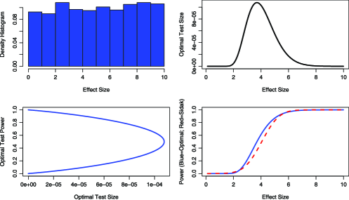
Figure 1: Optimal test sizes and powers for $2\mbox{,}000$ MP tests of hypotheses under normality when the effect sizes were generated from a $\operatorname{uniform}[0.1,10]$ distribution. Panel four shows the powers for both the optimal [solid black] and the Šidák [dashed red] tests with respect to effect sizes.

The efficiency of the optimal procedure relative to the Šidák procedure was measured via the ratio (multiplied by 100) of the average power over the $M$ tests, defined by $\sum_{m\in\mathcal{M}}\rho_{m}(\eta_{m})/M$, of the optimal procedure and the average power of the Šidák procedure. The fourth panel in Figure 1 depicts the powers of the resulting tests versus the effect size for both procedures (solid blue${}={}$optimal; dashed red${}={}$Šidák). For these uniformly-generated effect sizes, the efficiency of the optimal procedure over the Šidák is 103.5%. This efficiency is affected by the vector of effect sizes. For instance, when we change the effect sizes in Figure 1 to be generated from a uniform over $[0.1,2]$, then the efficiency jumps to 181.7%, though it should also be pointed out that since the effect sizes are small, then the overall powers of both procedures are also small.

4.5 A size-investing strategy

In the preceding Gaussian example, as well as in other situations we examined, for example, with exponential and Bernoulli distributions, we observed the phenomenon where, among the $M$ tests, those with low powers (small effect sizes) and those with high powers (large effect sizes) are allocated relatively small sizes in the weak FWER-controlling optimal procedure. The tests with larger sizes are those with moderate powers or effect sizes. This is a size-investing strategy in the multiple hypotheses testing problem, and it has intuitive content. With the overall goal of making more real discoveries while controlling the proportion of false discoveries for a pre-specified, usually small, overall size $\alpha$, the optimal procedure dictates that not much size should be accorded those tests with either very low or very high powers. The former case will not lead to any discoveries anyway if the size that could be allocated is small, while the latter case will lead to discoveries even if the test sizes are made small. Thus, there is more to be gained by investing larger sizes on those tests that are of moderate powers, and an appropriate tweaking of their test sizes according to condition (i) in Theorem 4.3 improves the ability to achieve more real discoveries. However, this phenomenon is dependent on the magnitude of the overall size. If this overall size is made larger, more leeway ensues to the extent that it may then be more beneficial to allocate more size to those with low powers since those tests with moderate powers, when they had small sizes, may now have larger powers because of the consequent increase in their sizes. The precise and crucial determinant of where the differential sizes should be allocated are the rates of change of the ROC functions, with some size-attenuation. Interesting discussions of size and weight allocation strategies can also be found in WesKriYou98 , where the size allocation was related to the “$\alpha$-spending” function of LandeM83 , in FosSti08 which deals with $\alpha$-investing in sequential procedures that control expected false discoveries, and in GenRoeWas06 , RoqWie09 which discuss optimal weights for the $p$-values.

A tangential real-life manifestation of this strategy occurred during the 2008 American presidential election, with the total resources (financial, manpower, etc.) available to the candidates analogous to the overall size in the multiple testing problem. In the waning days of the campaign, the major candidates, then-Senator Barack Obama of the Democratic Party and Senator John McCain of the Republican Party, focused their campaign efforts, in terms of allocating their financial and manpower resources, in the “battleground states” of North Carolina, Virginia and Pennsylvania, while basically ignoring the “in-the-bag states” of South Carolina, then expected to vote for McCain, and California, then expected to vote for Obama. Also, by virtue of the deep resources of the Obama campaign, it was able to allocate more resources even in states that traditionally voted Republican, whereas the McCain campaign, with a relatively smaller war chest, had to “drop” some states (e.g., Michigan) in their campaign. The behaviors of the two camps somehow mirror the size-investing strategy with proper accounting of each campaign’s overall resources.

5 Restrictions, extensions and connections

5.1 On the restriction to $\mathcal{D}_{0}$

The optimization problem for weak FWER control could be construed as limited since we restricted to the subclass $\mathcal{D}_{0}$ thus leading to an optimal weak FWER-controlling procedure that is still simple. In Sto07 , SunCai07 , it was demonstrated that performance is enhanced via compound MDFs. Examples of compound MDFs are the estimated optimal discovery procedure (ODP) in Sto07 , StoDaiLee07 , the FDR-controlling procedure in BenHoc95 , and the oracle-based adaptive MDFs in SunCai07 .

Could we immediately start from compound MDFs in the search for an optimal weak FWER-controlling compound MDF? Let us suppose that $\bolds{\delta}=(\delta_{m}\dvtx m\in\mathcal{M})$ is a compound MDF, so $\delta_{m}$ depends on $({X},{U})$ and not only on $(X_{m},U_{m})$. For such an MDF, we have

$$R_{0}(\bolds{\delta},Q)=\mathbf{P}_{Q}\biggl{\{}\bigcup_{m\in\mathcal{M}_{0}(Q)}[\delta_{m}({X},{U})=1]\biggr{\}}.$$ (17)

Now, even if the independence Condition (I) holds, $(\delta_{m}({X},{U})\dvtx m\in\mathcal{M}_{0}(Q))$ need not be an independent collection. As such no closed-form exact expression for $R_{0}(\bolds{\delta},Q)$ need exist. The right-hand side in (17) could be Bonferroni-bounded by

$$\operatorname{EFP}(\bolds{\delta},Q)\equiv\sum_{m\in\mathcal{M}_{0}(Q)}\alpha_{\delta_{m}}(Q),$$ (18)

called the expected number of false positives in Sto07 . Alternatively, if a generalized positive quadrant dependence (PQD) condition holds, with

$$\mathbf{P}_{Q}\biggl{\{}\bigcap_{m\in\mathcal{M}_{0}(Q)}[\delta_{m}({X},{U})=0]\biggr{\}}\geq\prod_{m\in\mathcal{M}_{0}(Q)}\mathbf{P}_{Q}\{\delta_{m}({X},{U})=0\},$$

then the right-hand side in (17) could be upper-bounded by

$$\operatorname{PQD}(\bolds{\delta},Q)\equiv 1-\prod_{m\in\mathcal{M}_{0}(Q)}[1-\alpha_{\delta_{m}}(Q)],$$ (19)

where $\alpha_{\delta_{m}}(Q)=E_{Q}\delta_{m}({X},{U})$, the size of $\delta_{m}$ when $m\in\mathcal{M}_{0}(Q)$. For this compound MDF, its MDR is $R_{2}(\bolds{\delta},Q)={\sum_{m\in\mathcal{M}_{1}(Q)}[1-\pi_{\delta_{m}}(Q)]}$, where $\pi_{\delta_{m}}(Q)=E_{Q}\delta_{m}({X},{U})$ is the power of $\delta_{m}$ when $m\in\mathcal{M}_{1}(Q)$.

An optimization approach could proceed by putting an upper threshold $\alpha\in(0,1)$ on either (18) or (19), and then finding the $\bolds{\delta}$ that minimizes $R_{2}(\bolds{\delta},Q)$, or equivalently, maximizes $\operatorname{ETP}(\bolds{\delta},Q)\equiv\sum_{m\in\mathcal{M}_{1}(Q)}\pi_{\delta_{m}}(Q)$, the latter quantity referred to as the expected number of true positives in Sto07 . The MDFs in Spj72 and Sto07 were both obtained through this program. The MDF in Spj72 is

$$\bolds{\delta}_{\mathrm{SPJ}}(\alpha)=\mathop{\arg\max}_{\bolds{\delta}\in\mathcal{D}_{0}}\{\operatorname{ETP}(\bolds{\delta},Q_{1})\dvtx\operatorname{EFP}(\bolds{\delta},Q_{0})\leq\alpha\},$$ (20)

where $Q_{0}\in\mathcal{Q}_{0}$ and $Q_{1}\in\mathcal{Q}_{1}$; whereas the optimal discovery procedure (ODP) in Sto07 is

$$\bolds{\delta}_{\mathrm{STO}}(\alpha;Q)=\mathop{\arg\max}_{\bolds{\delta}\in\mathcal{D}}\{\operatorname{ETP}(\bolds{\delta},Q)\dvtx\operatorname{EFP}(\bolds{\delta},Q)\leq\alpha\},$$ (21)

where $Q$ is the true probability measure of ${X}$. The use of EFP as type I error measure in Sto07 enabled a calculus of variations optimization to obtain the ODP. This has a particularly interesting structure when we utilize as its input the vector of $p$-value statistics $(S_{m}^{*}(x_{m},u_{m})\dvtx m\in\mathcal{M})$ from the MP MDP $\bolds{\Delta}^{*}=(\Delta_{m}^{*}\dvtx m\in\mathcal{M})$ with multiple decision size function $\mathbf{A}_{\bolds{\Delta}^{*}}^{*}=\{(A_{m}^{*}(\eta)\dvtx\eta\in[0,1])\dvtx m\in\mathcal{M}\}$ and multiple decision ROC function $\bolds{\rho}_{\bolds{\Delta}^{*}}^{*}=\{(\rho_{m}^{*}(\eta)\dvtx\eta\in[0,1])\dvtx m\in\mathcal{M}\}$ and with $A_{m}^{*}(\cdot)$ and $\rho_{m}^{*}(\cdot)$ both differentiable with derivatives $(A_{m}^{*})^{\prime}(\cdot)$ and $(\rho_{m}^{*})^{\prime}(\cdot)$. The significance thresholding function $\mathcal{S}\dvtx([0,1],\sigma[0,1])\rightarrow(\Re,\sigma(\Re))$ utilized in the ODP becomes

$$\mathcal{S}(s;Q)=\frac{\sum_{m\in\mathcal{M}_{1}(Q)}(\rho_{m}^{*})^{\prime}(s)}{\sum_{m\in\mathcal{M}_{0}(Q)}(A_{m}^{*})^{\prime}(s)},$$ (22)

a consequence of Lemma 2 in Sto07 and Proposition 3.2. The ODP $\bolds{\delta}_{\mathrm{STO}}=(\delta_{m,\mathrm{STO}}\dvtx m\in\mathcal{M})$ has a single-thresholding structure with components

$$\delta_{m,\mathrm{STO}}(S_{m}^{*}(x_{m},u_{m});Q)=I\{\mathcal{S}(S_{m}^{*}(x_{m},u_{m});Q)\geq\lambda\},\qquad m\in\mathcal{M},$$

where $\lambda\in[0,\infty)$ is chosen so the size constraint on $\operatorname{EFP}(\bolds{\delta}_{\mathrm{STO}}(\alpha;Q),Q)$ is approximately satisfied. Observe that each of these components is still of simple-type, unless $\lambda$ is determined in a data-dependent manner using the full data $({x},{u})$. Note also that $\bolds{\delta}_{\mathrm{STO}}$ was derived under complete knowledge of the unknown $Q$, or more specifically, the sets $\mathcal{M}_{0}(Q)$ and $\mathcal{M}_{1}(Q)$, as can be seen in (22), hence is referred to as an oracle MDF. For the simple null versus simple alternative hypotheses case, the size functions $A_{m}^{*}(\cdot)$’s and the ROC functions $\rho_{m}^{*}(\cdot)$’s will be known, but with composite hypotheses they will be unknown. To implement $\bolds{\delta}_{\mathrm{STO}}$, it was proposed in Sto07 , StoDaiLee07 that these unknown quantities, sets, functions, or significance thresholding function, be estimated using the data $({x},{u})$. This will make the estimated ODP of compound type. But note that through this plug-in approach the exact optimality property of the ODP need not anymore hold for the estimated version; see also SunCai07 , FerFriRueThoKon08 . In contrast, $\bolds{\delta}_{\mathrm{SPJ}}$ is determined only by the two classes of extreme probability measures, $\mathcal{Q}_{0}$ and $\mathcal{Q}_{1}$, so the marginal probability measures, $Q_{m}$’s, are completely known, and not by the unknown true probability measure $Q$ governing $X$. This fact was criticized in Sto07 as a “potentially problematic optimality” criterion. More importantly, it should be recognized that both $\bolds{\delta}_{\mathrm{SPJ}}$ and $\bolds{\delta}_{\mathrm{STO}}$ need not be the optimal weak or strong FWER- or FDR-controlling MDFs since the Bonferroni upper bound for $R_{0}(\bolds{\delta},Q)$ utilized in their derivations is hardly a sharp upper bound.

The criticism leveled against $\bolds{\delta}_{\mathrm{SPJ}}$ could also be invoked against our optimal weak FWER-controlling procedure since we also relied on a criterion determined only by the extreme classes $\mathcal{Q}_{0}$ and $\mathcal{Q}_{1}$. However, note that each component of the optimal weak FWER-controlling multiple decision size vector, and consequently each component of $\bolds{\delta}_{W}^{*}(\alpha)$, uses all of the $Q_{m0}$’s and $Q_{m1}$’s, analogously to the ODP, though the MDF $\bolds{\delta}_{W}^{*}(\alpha)$ is still neither adaptive nor compound. Our development of this simple MDF, which is optimal in the class $\mathcal{D}_{0}$, is a prelude to our development of adaptive and compound MDFs strongly-controlling FWER and FDR. The MDF $\bolds{\delta}_{W}^{*}(\alpha)$ will be the anchor for these FWER and FDR strongly-controlling compound MDFs. These new MDFs are discussed in Section 6 for strong FWER-control and in Section 7 for FDR control. Our approach to obtaining these strongly-controlling MDFs is indirect, whereas that in Sto07 is direct. There is also an intrinsic difference in the problems considered since our focus is on the type I error risk functions $R_{0}$ and $R_{1}$, whereas in Spj72 , Sto07 the simpler type I error metric of EFP was utilized. Looking forward, though our starting point is the optimal weak FWER-controlling simple MDF $\bolds{\delta}_{W}^{*}(\alpha)$, there is confidence in the viability of our indirect approach to generate good MDFs since we will establish later that both the sequential Šidák procedure and the BH procedure are special cases of our new MDFs under exchangeability.

5.2 Families with MLR property

The initial simplification to the simple null versus simple alternative hypotheses for each $m\in\mathcal{M}$ could be perceived as a limitation because of the need to know the $Q_{m1}$’s to determine the ROC functions. However, this approach, which was also implemented in Spj72 , Sto07 , RoqWie09 , is natural and historically-justified by the Neyman–Pearson framework. We surmise that in this multiple decision problem, the solution to the simple null versus simple alternative hypotheses setting will play a prominent role in solving the composite hypotheses setting, since it appears that for an MDF to possess optimality, it will require knowledge, either in exact, approximate, or estimated forms, of the alternative hypotheses distributions. We touch on this aspect in the presence of the monotone likelihood ratio (MLR) property; see Leh97 .

Suppose that for each $m\in\mathcal{M}$, the density function $q_{m}$ belongs to a one-dimensional parametric family $\mathcal{F}_{m}=\{q_{m}(\cdot;\xi_{m})\dvtx\xi_{m}\in\Gamma_{m}\subset\Re\}$ which possesses the MLR property. A typical pair of hypotheses to be tested would be $H_{m0}^{*}\dvtx\xi_{m}\leq\xi_{m0}$ versus $H_{m1}^{*}\dvtx\xi_{m}>\xi_{m0}$, where $\xi_{m0}$ is known. With the MLR property, a uniformly most powerful (UMP) test function $\delta_{m}(X_{m},U_{m};\eta_{m})$ of size $\eta_{m}$ exists, with this UMP test identical to the MP test of size $\eta_{m}$ for the simple null hypothesis $H_{m0}\dvtx\xi_{m}=\xi_{m0}$ versus the simple alternative hypothesis $H_{m1}\dvtx\xi_{m}=\xi_{m1}$, with $\xi_{m1}>\xi_{m0}$. When dealing with the single-pair hypothesis testing problem, recall that exact knowledge of the value of $\xi_{1}$ is not necessary since the critical constants of the size-$\eta$ MP test for $H_{0}\dvtx\xi=\xi_{0}$ versus $H_{1}\dvtx\xi=\xi_{1}$ can be made independent of $\xi_{1}$. In contrast, for the multiple decision problem, to determine the optimal size allocations for each of the $M$ MP tests, the powers of the tests at the $\xi_{m1}$’s are required, hence the need to know the values of the $\xi_{m1}$’s. When $M$ is large, such information may not be so forthcoming. The default procedure is the simplistic approach of simply assuming that the $(Q_{m0},Q_{m1})$ is invariant in $m$, which is the exchangeable setting. However, this exchangeable assumption is most likely wrong as a consequence of varied effect sizes or different test functions utilized. See, for instance, EfrAAS08 for real situations where exchangeability do not hold. We propose two possible solutions to this dilemma.

The first approach is to solicit from the scientific investigator the values of the $\xi_{m1}$’s for which the powers are of most interest. Such values may coincide with those that are scientifically different from the $\xi_{m0}$’s. Such elicitation, which may not be very feasible in practice if $M$ is large, but which may be made possible by forming subclasses or clusters of the $M$ genes as in EfrAAS08 , amounts to specifying effect sizes. Formation of such clusters must be made in close consultation with the investigator, or perhaps guided by the result of a preliminary cluster analysis using data independent of that used in the decision functions. For the specified $\xi_{m1}$’s, the ROC functions in the determination of the optimal weak FWER-controlling multiple size vector become $\rho_{m}(\eta)=\pi_{\delta_{m}^{*}(\eta)}(\xi_{m1})$ for $m\in\mathcal{M}$, where $\delta_{m}^{*}(\eta)$ is the simple MP test of size $\eta$ for testing $H_{m0}\dvtx\xi_{m}=\xi_{m0}$ versus $H_{m1}\dvtx\xi_{m}=\xi_{m1}$, and $\pi_{\delta_{m}^{*}(\eta)}(\xi_{m1})$ is the power of $\delta_{m}^{*}(\eta)$ (at $\xi_{m}=\xi_{m1}$). In the clustered situation with $\mathcal{M}=\biguplus_{k=1}^{K}\mathcal{M}_{k}$, we may denote by $\bar{\rho}_{k}(\eta)$ and $\zeta_{k}$, respectively, the common ROC function and size for the decision functions in cluster $\mathcal{M}_{k}$. Under second-order differentiability of $\bar{\rho}_{k}(\eta)$’s, by Theorem 4.3, the optimal weak FWER-$\alpha$ controlling multiple size vector $\zeta(\alpha)=(\zeta_{1}(\alpha),\zeta_{2}(\alpha),\ldots,\zeta_{K}(\alpha))$ is the $\zeta=(\zeta_{1},\zeta_{2},\ldots,\zeta_{K})$ that solves the set of equations $\forall k=1,2,\ldots,K\dvtx\bar{\rho}_{k}^{\prime}(\zeta_{k})(1-\zeta_{k})=\lambda$ for some $\lambda\in\Re_{+}$ with $\sum_{k=1}^{K}|\mathcal{M}_{k}|\log(1-\zeta_{k})=\log(1-\alpha)$.

The second approach, analogous to those in WesKriYou98 , RubDudLaa06 , SunCai07 , Sto07 , StoDaiLee07 , KanYeLiuAllGao09 is to estimate or approximate the underlying values of the $\xi_{m}$’s either using the observed data $x$, possibly via shrinkage-type estimators, or through the use of prior information which could be informed by external covariates as in FerFriRueThoKon08 . Addressing this same restriction of requiring knowledge of the simple null and simple alternative hypotheses and advocating this second approach, RoqWie09 , page 679, stated: “although leading to oracle procedures, it can be used in practice as soon as the null and alternative distributions are estimated or guessed reasonably accurately from independent data.” By “independent data” is meant in RoqWie09 as data different from that used in performing the actual tests. However, such external data need not always be used for estimating or imputing the unknown parameters. For example, suppose that for each $m\in\mathcal{M}$, data $x_{m}$ could be partitioned into $(v_{m},w_{m})$. We may then use $\tilde{\xi}_{m}(v_{m})=\max\{\xi_{m0},\hat{\xi}_{m}(v_{m})\}$, where $\hat{\xi}_{m}(v_{m})$ is the maximum likelihood estimate of $\xi_{m}$ based on $v_{m}$, and proceed as in the preceding paragraph with $\xi_{m1}$ set to $\tilde{\xi}_{m}(v_{m})$ for each $m\in\mathcal{M}$, and with the component data $w_{m}$ used in the test functions. The resulting MDF will be of an adaptive type, possibly also compound as in SunCai07 if shrinkage estimators are used for estimating the $\xi_{m}$’s using the $v_{m}$ components. Observe that if for some $m_{0}\in\mathcal{M}$, $\tilde{\xi}_{m}(v_{m_{0}})$ and $\xi_{{m_{0}}0}$ are very close or identical, then a relatively small size will be allocated to the MP test for component $m_{0}$. This amounts to downgrading the testing problem for this component, a fact of importance since a criticism of multiple hypotheses testing, especially when using FDR, is that an unscrupulous investigator may keep adding irrelevant genes. When using the adaptive MDF arising from the optimal multiple decision size vector, this investigator’s strategy will backfire since the adaptive MDF will automatically downgrade the irrelevant genes. This second approach still requires deeper study. For instance, there is the issue of how to partition each $x_{m}$ into the $v_{m}$ and $w_{m}$ components. Furthermore, the impact of a misspecified $\xi_{m1}$, possibly arising from the estimation procedure, needs to be ascertained.

5.3 Connections to $p$-value statistics

Proposition 3.2 indicates that the ROC function $\eta\mapsto\rho_{m}(\eta)$ is differentiable if and only if the distribution function of the $p$-value statistic $S_{m}(X_{m},U_{m})$ under $H_{m1}\dvtx Q_{m}=Q_{m1}$ is differentiable. In this case, $\rho_{m}^{\prime}(\cdot)$ coincides with $h_{m}(\cdot)$, the density function of $S_{m}(X_{m},U_{m})$ under $H_{m1}\dvtx Q_{m}=Q_{m1}$. Condition (i) in Theorem 4.3 is equivalent to the constancy in $m$ of $h_{m}(\eta_{m})(1-\eta_{m})$. This is surprising since it indicates that it is not enough to simply find the sizes that maximize these $h_{m}(\cdot)$’s, as dictated by the Neyman–Pearson lemma when dealing with a single pair of null and alternative hypotheses. Rather, in the multiple hypotheses testing scenario, there is attenuation in that larger sizes incur penalties. Condition (i) in Theorem 4.3 governs the interactions among the $M$ tests regarding their size allocations to achieve the best overall result, in terms of overall type II error, among themselves.

The optimal weak FWER-controlling MDF can be converted to a procedure based on the $p$-value statistics. If $\bolds{\eta}^{*}(\alpha)=(\eta_{m}^{*}(\alpha),m\in\mathcal{M})$ is the optimal weak FWER-$\alpha$ multiple decision size vector and $(S_{m}(x_{m},u_{m}),m\in\mathcal{M})$ is the vector of computed $p$-value statistics, the decision based on data $(x,u)=((x_{m},u_{m}),m\in\mathcal{M})$ is $\delta^{*}(x,u)=(I\{S_{m}(x_{m},u_{m})\leq\eta_{m}^{*}(\alpha)\},m\in\mathcal{M})$, an MDF based on weighted $p$-values. This is related to the approach in several papers using weighted $p$-values such as GenRoeWas06 , WasRoe06 , RubDudLaa06 , KanYeLiuAllGao09 , RoqWie09 . In our case, the weights are tied-in to the optimal sizes.

6 Strong FWER control

Let $\bolds{\Delta}^{*}=(\Delta_{m}^{*},m\in\mathcal{M})$ be the MP MDP with $\Delta_{m}^{*}=(\delta_{m}^{*}(\eta)\dvtx\eta\in[0,1])$ the MP decision process for $H_{m0}\dvtx Q_{m}=Q_{m0}$ versus $H_{m1}\dvtx Q_{m}=Q_{m1}$ based on $(X_{m},U_{m})$. Wlog, assume that the size function $A_{m}(\cdot)$ of $\Delta_{m}^{*}$ satisfies $A_{m}(\eta)=\eta$. Define $\bolds{\eta}\dvtx[0,1]\rightarrow[0,1]^{M}$ such that $\bolds{\eta}(\alpha)=(\eta_{m}(\alpha),m\in\mathcal{M})$ is the optimal weak FWER-controlling multiple decision size vector at level $\alpha$. Assume that each component of this mapping is nondecreasing and continuous, which is the case when the ROC functions of $\bolds{\Delta}^{*}$ are twice-differentiable as established in Proposition 4.5.

For a weak FWER threshold of $\alpha\in[0,1]$, the optimal MDF in $\mathcal{D}_{0}$ is $\bolds{\delta}_{W}^{*}(\alpha)=(\delta_{m}^{*}(\eta_{m}(\alpha)),m\in\mathcal{M})$, as given in (12). Associated with this MDF is the generalized multiple decision $p$-value statistic $\mathbf{W}=(W_{m},m\in\mathcal{M})$, where

$$W_{m}\equiv W_{m}(X_{m},U_{m})=\inf\{\alpha\in[0,1]\dvtx\delta_{m}^{*}(\eta_{m}(\alpha))=1\}.$$ (23)

The $w_{m}=W_{m}(x_{m},u_{m})$ is the smallest weak FWER size leading to rejection of $H_{m0}$ when using $\bolds{\delta}_{W}^{*}(\alpha)$ given data $(x,u)=((x_{m},u_{m}),m\in\mathcal{M})$. The usual $p$-value statistic $S_{m}$ [see (3.2)] for $\delta_{m}^{*}$ is related to $W_{m}$ via

$$\forall m\in\mathcal{M}\dvtx S_{m}(X_{m},U_{m})=\eta_{m}(W_{m}(X_{m},U_{m})).$$ (24)

Now, a lá Sto07 , SunCai07 , suppose an Oracle knows $Q$, the true underlying probability measure of $X$. For the MDF $\bolds{\delta}_{W}^{*}(\alpha)$, its FWER is

$$R_{0}(\bolds{\delta}_{W}^{*}(\alpha),Q)=1-\prod_{m\in\mathcal{M}}[1-\eta_{m}(\alpha)]^{1-\theta_{m}(Q)}.$$

This is nondecreasing and continuous in $\alpha$ since the mappings $\alpha\mapsto\eta_{m}(\alpha)$ for each $m\in\mathcal{M}$ are nondecreasing and continuous. If the Oracle desires to control this type I error rate at a value $q^{*}\in[0,1]$ and also minimize the MDR given by $R_{2}(\bolds{\delta}_{W}^{*}(\alpha),Q)=|\mathcal{M}_{1}(Q)|-\sum_{m\in\mathcal{M}_{1}(Q)}\rho_{m}(\eta_{m}(\alpha))$, where $\rho_{m}(\eta_{m}(\alpha))$ is the power of $\delta_{m}^{*}(\eta_{m}(\alpha))$, then she should choose the largest $\alpha\in[0,1]$ such that $R_{0}(\bolds{\delta}_{W}^{*}(\alpha),Q)=q^{*}$. Owing to the continuity and nondecreasing properties of $R_{0}(\bolds{\delta}_{W}^{*}(\alpha),Q)$ in $\alpha$, the Oracle’s optimal $\alpha$ could also be expressed via

$$\alpha^{\dagger}(q^{*};Q)=\inf\biggl{\{}\alpha\in[0,1]\dvtx\prod_{m\in\mathcal{M}}[1-\eta_{m}(\alpha)]^{1-\theta_{m}(Q)}<1-q^{*}\biggr{\}}.$$

However, there is no Oracle and $Q$ is not known, else there is no multiple decision problem. Thus, $\alpha^{\dagger}(q^{*};Q)$ is not observable. A natural idea is to estimate the unknown $\theta_{m}(Q)$, the state of the $m$th pair of hypotheses. An intuitive and simple estimator of $\theta_{m}(Q)$ for a fixed value of $\alpha$ is

$$\widehat{\theta}_{m}(Q)=\delta_{m}^{*}(\eta_{m}(\alpha)-)\equiv\delta_{m}^{*}(X_{m},U_{m};\eta_{m}(\alpha)-).$$ (25)

In turn, we obtain a step-down estimator $\alpha^{\dagger}(q^{*})\equiv\alpha^{\dagger}(X,U;q^{*})$ of the Oracle-based $\alpha^{\dagger}(q^{*};Q)$ given by

$$\alpha^{\dagger}(q^{*})=\inf\biggl{\{}\alpha\in[0,1]\dvtx\prod_{m\in\mathcal{M}}[1-\eta_{m}(\alpha)]^{1-\delta_{m}^{*}(\eta_{m}(\alpha)-)}<1-q^{*}\biggr{\}}.$$ (26)

This determines a compound MDF $\bolds{\delta}_{S}^{*}(q^{*})\equiv\bolds{\delta}_{S}^{*}(X,U;q^{*})\in\mathcal{D}$, where

$$\bolds{\delta}_{S}^{*}(q^{*})=\bigl{(}\delta_{m}^{*}(\eta_{m}(\alpha^{\dagger}(q^{*}))),m\in\mathcal{M}\bigr{)}.$$ (27)

By virtue of the optimal choice of the $\eta_{m}(\alpha)$’s and the use of the MP tests, we expect $\bolds{\delta}_{S}^{*}(q^{*})$ to possess excellent, if not optimal, MDR-properties. By taking the infimum over the weak FWER-size $\alpha$ coupled with the estimation of $\theta_{m}(Q)$ by $\delta_{m}^{*}(\eta_{m}(\alpha)-)$ in (26), there occurs an adaptive downweighting of components whose $H_{m0}$’s are most likely correct as dictated by the data $(x,u)$. Theorem 6.1 below establishes that $\bolds{\delta}_{S}^{*}(q^{*})$ in (27) does strongly control the FWER.

Theorem 6.1.

Let $q^{*}\in[0,1]$. Then, $\forall Q\in\mathcal{Q}$, $R_{0}(\delta_{S}^{*}(q^{*}),Q)\leq q^{*}$.

Next, we reexpress $\bolds{\delta}_{S}^{*}(q^{*})$ in terms of the generalized $p$-value statistic $\mathbf{W}$. This is achieved by defining the random variable

$$J^{\dagger}(q^{*})=\max\Biggl{\{}j\in\mathcal{M}\dvtx\prod_{m=i}^{M}\bigl{[}1-\eta_{(m)}\bigl{(}W_{(i)}\bigr{)}\bigr{]}\geq 1-q^{*},i=1,2,\ldots,j\Biggr{\}}.$$

Since $\alpha^{\dagger}(q^{*})\in[W_{(J^{\dagger}(q^{*}))},W_{(J^{\dagger}(q^{*})+1)})$, then

$$\bolds{\delta}_{S}^{*}(q^{*})=\bigl{(}\delta_{m}^{*}\bigl{(}\eta_{m}\bigl{(}W_{(J^{\dagger}(q^{*}))}\bigr{)}\bigr{)},m\in\mathcal{M}\bigr{)}.$$

The next result shows that the sequential step-down Šidák MDF, which strongly controls FWER, is a special case of $\bolds{\delta}_{S}^{*}(q^{*})$ under exchangeability.

Proposition 6.1.

If the $M$ ROC functions are identical, then $\bolds{\delta}_{S}^{*}(q^{*})$ coincides with the sequential Šidák step-down FWER-controlling MDF.

7 Strong FDR control

Assume the same framework as in Section 6. Our idea in obtaining an FDR-controlling MDF builds on the development of the BH MDF, specifically the rationale of Theorem 2 in BenHoc95 . Let $q^{*}\in[0,1]$ be the desired FDR threshold and $Q$ be the underlying probability measure of $X$. We introduce two stochastic processes: $\mathbf{T}_{0}=\{T_{0}(\alpha;Q)\dvtx\alpha\in[0,1]\}$ and $\mathbf{T}=\{T(\alpha)\dvtx\alpha\in[0,1]\}$, where

$$T_{0}(\alpha;Q)=\sum_{m\in\mathcal{M}_{0}(Q)}\delta_{m}^{*}(\eta_{m}(\alpha))\quad\mbox{and}\quad T(\alpha)=\sum_{m\in\mathcal{M}}\delta_{m}^{*}(\eta_{m}(\alpha)).$$

For the MDF $\delta_{W}^{*}(\alpha)$, its FDR is

$$R_{1}(\delta_{W}^{*}(\alpha),Q)=E_{Q}\biggl{\{}\frac{T_{0}(\alpha;Q)}{T(\alpha)}I\{T(\alpha)>0\}\biggr{\}}.$$

By the definition of the generalized $p$-value statistics $W_{m}$’s in (23), we have for $\alpha\in[W_{(m)},W_{(m+1)})$ that $T(\alpha)=m$, whereas

$$E_{Q}\{T_{0}(\alpha;Q)\}=\sum_{m\in\mathcal{M}}\bigl{(}1-\theta_{m}(Q)\bigr{)}\eta_{m}(\alpha)\leq\sum_{m\in\mathcal{M}}\eta_{m}(\alpha).$$ (28)

Focus now on an $\alpha\in[W_{(m)},W_{(m+1)})$. If $\sum_{j\in\mathcal{M}}\eta_{j}(W_{(m)})\leq mq^{*}$, then the best $\alpha$ in this interval will be the largest value satisfying $\sum_{j\in\mathcal{M}}\eta_{j}(\alpha)\leq mq^{*}$, since by increasing $\alpha$, the MDR decreases as argued in the development of $\delta_{S}^{*}(q^{*})$ in Section 6. This motivates our definition of $\alpha^{*}(q^{*})=\alpha^{*}(X,U;q^{*})$ as the step-up estimator

$$\alpha^{*}(q^{*})=\sup\biggl{\{}\alpha\in[0,1]\dvtx\sum_{m\in\mathcal{M}}\eta_{m}(\alpha)\leq q^{*}\sum_{m\in\mathcal{M}}\delta_{m}^{*}(\eta_{m}(\alpha))\biggr{\}}.$$ (29)

This induces a compound MDF $\bolds{\delta}_{F}^{*}(q^{*})\equiv\bolds{\delta}_{F}^{*}(X,U;q^{*})\in\mathcal{D}$ given by

$$\bolds{\delta}_{F}^{*}(q^{*})=\bigl{(}\delta_{m}^{*}(\eta_{m}(\alpha^{*}(q^{*}))),m\in\mathcal{M}\bigr{)}.$$ (30)

Theorem 7.1 establishes that $\bolds{\delta}_{F}^{*}(q^{*})$ does control the FDR at $q^{*}$. Interestingly, the proof of this theorem, which can be found in PenHabWu10Supp , employs a reverse martingale argument.

Theorem 7.1.

Let $q^{*}\in[0,1]$. If, $\forall Q\in\mathcal{Q}\setminus\{Q_{0}\}$ and $\forall\alpha\in(0,1)$,$|\mathcal{M}_{0}(Q)|\max_{m\in\mathcal{M}_{0}(Q)}\eta_{m}(\alpha)\leq\sum_{m\in\mathcal{M}}\eta_{m}(\alpha)$, then $R_{1}(\bolds{\delta}_{F}^{*}(q^{*}),Q)\leq q^{*}$ for $\forall Q\in\mathcal{Q}$.

Some remarks are in order regarding the condition in Theorem 7.1. Clearly, the Šidák multiple decision size vector, which is the optimal multiple decision size vector when the ROC functions are identical, always satisfies this condition. When not in this exchangeable setting, this condition induces some control on the differences of the ROC functions. The next proposition establishes that the BH procedure is a special case of $\bolds{\delta}_{F}^{*}(q^{*})$ under exchangeability.

Proposition 7.1.

If the ROC functions are identical, then $\bolds{\delta}_{F}^{*}(q^{*})$ is the FDR-$q^{*}$ controlling MDF in BenHoc95 .

Examination of the proof of Proposition 7.1 as presented in PenHabWu10Supp shows that the BH MDF $\bolds{\delta}^{\mathrm{BH}}(q^{*})$ coincides with the Šidák-size based MDF $\bolds{\delta}^{S}(q^{*})$. The martingale proof for Theorem 7.1 thus carries over to establishing FDR control by $\bolds{\delta}^{\mathrm{BH}}(q^{*})$. We mention that a martingale-based proof of FDR control by $\bolds{\delta}^{\mathrm{BH}}(q^{*})$ has also been presented in StoTaySie04 .

We also provide an alternative form of $\bolds{\delta}_{F}^{*}(q^{*})$ in terms of the generalized $p$-value statistics $W_{m}$’s, a form analogous to the conventional formulation of the BH procedure. Define

$$J^{*}(q^{*})\equiv J^{*}(X,U;q^{*})=\max\Biggl{\{}m\in\mathcal{M}\dvtx\sum_{j\in\mathcal{M}}\eta_{j}\bigl{(}W_{(m)}\bigr{)}\leq q^{*}m\Biggr{\}}.$$ (31)

Then, it is easy to see that $\bolds{\delta}_{F}^{*}(q^{*})$ rejects $H_{(m)0}$ for $m\in\{1,2,\ldots,J^{*}(q^{*})\}$ and accepts $H_{(m)0}$ for $m\in\{J^{*}(q^{*})+1,J^{*}(q^{*})+2,\ldots,M\}$.

Finally, let us examine further the generalized $p$-value statistics $W_{m}$’s. Focusing on $W_{(1)}$, under $Q_{0}$, we have that, for $a\in(0,1)$,

$$\mathbf{P}_{Q_{0}}\bigl{(}W_{(1)}>a\bigr{)}=\mathbf{P}_{Q_{0}}\biggl{\{}\bigcap_{m\in\mathcal{M}}[\delta_{m}^{*}(\eta_{m}(a))=0]\biggr{\}}=\prod_{m\in\mathcal{M}}[1-\eta_{m}(a)]=1-a,$$

the second equality obtained by using the independence of the $\delta_{m}^{*}$’s under $Q_{0}$. Thus, $W_{(1)}$ is standard uniform when all null hypotheses are correct. Using this uniformity result and Lemma D.2 presented in PenHabWu10Supp dealing with lower and upper bounds of $\eta_{\bullet}$ for $\eta\in UB(C_{\alpha})$, we obtain in Proposition 7.2 presented below a lower bound for $R_{1}(\delta_{F}^{*}(q^{*}),Q_{0})$, the FDR when all the null hypotheses are correct.

Proposition 7.2.

$\forall q^{*}\in[0,1]$, $1-(1-q^{*}/M)^{M}\leq R_{1}(\delta_{F}^{*}(q^{*}),Q_{0})\leq q^{*}$.

8 A modest simulation

We compared through computer simulations the performances of $\bolds{\delta}_{F}^{*}$ and $\bolds{\delta}^{\mathrm{BH}}$ in terms of FDR and MDR. The simulation model utilized is similar to the Gaussian example illustrating the optimal weak FWER-controlling procedure in Section 4.4. In this model, the observables are $X_{m}\sim N(\mu_{m},1)$ for each $m\in\mathcal{M}$, which are independent of each other. The $m$th pair of hypotheses is $H_{m0}\dvtx\mu_{m}\leq 0$ versus $H_{m1}\dvtx\mu_{m}>0$. The UMP size-$\eta_{m}$ test is $\delta_{m}^{*}(X_{m};\eta_{m})=I\{X_{m}>\Phi^{-1}(1-\eta_{m})\}$. The true values of the means $\mu_{m}$’s are $\mu_{m}=\xi_{m}\theta_{m},m\in\mathcal{M}$, with $\theta_{m}\sim\operatorname{Ber}(p)$ and effect sizes $\xi_{m}\sim|N(\nu,1)|$, again independently generated from each other. The parameter combinations were induced by taking $M\in\{20,50,100\}$, $p\in\{0.1,0.2,0.4\}$ and $\nu\in\{1,2,4\}$. The FDR-threshold utilized were $q^{*}\in\{0.05,0.10\}$. Since the computational implementation of $\bolds{\delta}_{F}^{*}$ takes time, for each combination of $(q^{*},M,\nu,p)$, we limited our simulations to 1,000 replications. The simulated FDR and MDR^∗ were the averages of the false discovery proportions, $L_{1}(a,Q)$’s, and the standardized missed discovery proportions, $L_{2}(a,Q)/|\mathcal{M}_{1}(Q)|$, over the 1,000 replications. We used this standardized MDR since, for each replicate, a $Q$ is generated, hence $|\mathcal{M}_{1}(Q)|$ differs over the replications. In essence, we are comparing the averages of $R_{2}(\delta_{F}^{*},Q)/|\mathcal{M}_{1}(Q)|$ and $R_{2}(\delta^{\mathrm{BH}},Q)/|\mathcal{M}_{1}(Q)|$, where the averaging is with respect to the mechanism generating the $Q$’s over the simulation replications.

We only report results for $q^{*}=0.10$ in Table 1 since results for $q^{*}=0.05$ lead to similar conclusions. From this table, we observe that both $\bolds{\delta}_{F}^{*}$ and $\bolds{\delta}^{\mathrm{BH}}$ fulfill the FDR-constraint, and in a conservative manner, which is expected from theory. More importantly, the MDR-performance of $\bolds{\delta}_{F}^{*}$ is better compared to that of $\bolds{\delta}^{\mathrm{BH}}$, with this dominance holding for all twenty-seven parameter combinations. Observe that as $M$ is increased with $(\nu,p)$ remaining the same, there is an increase in their MDR^∗’s; whereas, when $\nu$ is increased, which increases the effect sizes, their MDR^∗’s decrease. Interestingly, the impact of a change of value in $p$, the proportion of true alternative hypotheses, did not necessarily translate into a monotone change in their MDR^∗’s, especially when $M=20$, though for the larger $M$-values, the change in MDR^∗ appears monotonically decreasing.

Table 1: Comparison of the false discovery rate (FDR) and standardized missed discovery rate (MDR^∗) performance of MDFs $\delta_{F}^{*}$ and $\delta^{\mathrm{BH}}$ under a variety of simulation parameters. This table is for $q^{*}=0.10$. The FDR and MDR^∗ are in percentages. The number of replications is 1,000

	$\bolds{q^{*}}$	$\bolds{M}$	$\bolds{\nu}$	$\bolds{p}$	$\bolds{\delta_{F}^{*}}$-FDR	$\bolds{\delta_{F}^{*}}$-MDR$\bolds{{}^{*}}$	$\bolds{\delta^{\mathrm{BH}}}$-FDR	$\bolds{\delta^{\mathrm{BH}}}$-MDR$\bolds{{}^{*}}$
$1$	0.1	$20$	1	0.1	8.03	$70.80$	$8.43$	$72.64$
$2$	0.1	$20$	1	0.2	7.55	$79.64$	$8.77$	$81.99$
$3$	0.1	$20$	1	0.4	6.05	$77.47$	$6.65$	$80.30$
$4$	0.1	$20$	2	0.1	7.70	$54.42$	$8.43$	$55.80$
$5$	0.1	$20$	2	0.2	7.39	$56.32$	$7.59$	$57.31$
$6$	0.1	$20$	2	0.4	6.47	$47.82$	$6.21$	$49.38$
$7$	0.1	$20$	4	0.1	9.14	$8.62$	$9.48$	$10.30$
$8$	0.1	$20$	4	0.2	7.80	$7.34$	$6.97$	$9.20$
$9$	0.1	$20$	4	0.4	6.15	$3.58$	$5.65$	$5.53$
$10$	0.1	$50$	1	0.1	8.83	$84.87$	$9.26$	$87.05$
$11$	0.1	$50$	1	0.2	7.11	$83.49$	$7.14$	$86.65$
$12$	0.1	$50$	1	0.4	6.45	$78.91$	$6.42$	$82.30$
$13$	0.1	$50$	2	0.1	8.36	$63.36$	$8.99$	$65.04$
$14$	0.1	$50$	2	0.2	8.74	$57.30$	$8.73$	$58.93$
$15$	0.1	$50$	2	0.4	5.80	$48.71$	$5.93$	$50.21$
$16$	0.1	$50$	4	0.1	8.84	$10.28$	$8.93$	$12.09$
$17$	0.1	$50$	4	0.2	7.93	$6.91$	$7.81$	$8.79$
$18$	0.1	$50$	4	0.4	6.34	$3.40$	$6.07$	$5.68$
$19$	0.1	$100$	1	0.1	9.14	$87.10$	$9.02$	$90.02$
$20$	0.1	$100$	1	0.2	8.21	$84.05$	$8.78$	$87.38$
$21$	0.1	$100$	1	0.4	5.92	$80.12$	$5.88$	$83.73$
$22$	0.1	$100$	2	0.1	9.79	$66.10$	$9.24$	$67.93$
$23$	0.1	$100$	2	0.2	7.68	$58.25$	$7.94$	$59.93$
$24$	0.1	$100$	2	0.4	5.74	$49.29$	$6.10$	$50.90$
$25$	0.1	$100$	4	0.1	8.37	$10.44$	$8.62$	$12.36$
$26$	0.1	$100$	4	0.2	7.72	$5.93$	$7.81$	$8.22$
$27$	0.1	$100$	4	0.4	5.69	$3.80$	$6.14$	$5.72$

It may appear from this simulation study that the standardized improvement of $\delta_{F}^{*}$ over $\delta^{\mathrm{BH}}$ is minuscule. However, note that when translated to overall number of discoveries, when $M$ is large, $\delta_{F}^{*}$ will lead to many more discoveries than $\delta^{\mathrm{BH}}$ while still maintaining desired FDR control. Such an increase in the number of discoveries may have important practical implications, such as enlarging the number of genes to be explored in consequent studies. This may translate to enhanced chances of discovering crucial and important genes without sacrificing the type I error rate.

9 Summary and concluding remarks

This paper provides some resolution on the role of the individual powers of test or decision functions, more appropriately their ROC functions, in multiple hypotheses testing problems. The importance and relevance of these problems have arisen because of the proliferation of high-dimensional “large $M$, small $n$” data sets in the natural, medical, physical, economic and social sciences. Such data sets are being created or generated due to advances in high-throughput technology, the latter fueled by speedy developments in computer technology and miniaturization.

Almost a century ago, Neyman and Pearson demonstrated the need to take into account the power function and the alternative hypothesis configuration when seeking an optimal test procedure in single-pair hypothesis testing. Their work led to a divorce from the then-existing significance or $p$-value approach. Currently, many multiple hypotheses testing procedures, epitomized by the Šidák procedures for weak and strong FWER control and by the Benjamini–Hochberg (BH) procedure for FDR control, are based on the $p$-values of the individual tests and do not consider differences in the power traits of the individual tests. They are appropriate in so-called exchangeable settings wherein power characteristics of the individual tests are identical. Such settings, however, are more the exception than the rule, since nonidentical power characteristics easily arise due to differences in the effect sizes, the dispersion parameters, or the test functions that are employed.

This paper examined whether differences in power characteristics of the individual tests could be exploited to improve on existing procedures for FWER and FDR control. Procedures were developed under the historically most fundamental scenario where the null and the alternative hypotheses are simple. First, an optimal MDF within the class of simple MDFs was shown to exist for weak FWER control. This MDF is better than the Šidák weak FWER-controlling MDF, though the latter is a special case of the optimal MDF under exchangeability. Optimality also informs us of an optimal size-investing strategy. Second, by using this optimal, though still restricted, MDF as an anchor, a compound MDF strongly controlling FWER was obtained. The sequential Šidák MDF is a special case of this MDF under exchangeability. Third, we developed a compound MDF that controls FDR. The BH procedure obtains from this MDF under exchangeability. By construction, these new MDFs have smaller MDRs relative to those that did not exploit power differences. The improvement was demonstrated through a modest simulation study by comparing the new FDR-controlling MDF and the BH MDF.

Though the proposed MDFs do improve on existing ones, we could not claim that they are optimal among all compound MDFs for strong FWER or FDR control. This question of global optimality is a difficult and elusive one. So far none of the existing compound MDFs, such as the estimated ODP in Sto07 , could claim global optimality. In our case, the possible drawback is that in constructing the new MDFs, we started with the class of simple MDFs. The resulting MDFs are indeed compound, but establishing global optimality is not transparent. A question even arise as to whether there truly exists an optimal MDF among all compound MDFs that, say, control FDR. One thing certain about our MDFs is that they do control FWER or FDR. This is in contrast to some MDFs that are obtained from oracle MDFs via plugging-in of estimates for unknown quantities. Even though the oracle MDF, which are unimplementable, satisfies the type I error rate control, the plug-in step will usually invalidate such control. See SunCai07 where optimality was in an asymptotic sense and with the type I error rate being the mFDR, as well as FerFriRueThoKon08 , RoqWie09 for more discussions on these issues.

A natural layer to add in the decision-theoretic formulation of the problem is a Bayesian layer where a prior measure is specified on the unknown probability measure $Q$ or, alternatively, on $\theta(Q)$. There is a possibility that through this Bayesian approach, one may be able to obtain a characterization of the class of optimal MDFs controlling type I error rates, or when the two types of error rates are combined, for example, via a weighted linear combination. The papers MulParRobRou04 , SarZhoGho08 , Efr08 , EfrAAS08 which employ Bayes or empirical Bayes approaches are highly relevant on this front.

Finally, we mention that there are still other aspects of the multiple decision problem not dealt with in this paper. First is the extension to situations with composite null and alternative hypotheses. We indicated some ideas in Section 5.2 for distributional models possessing the MLR property, but further and more extensive studies are needed. Second are possible dependencies among the components in $(X_{m},m\in\mathcal{M}_{0}(Q))$. We have assumed that this is an independent collection, but it is certainly of theoretical and applied relevance to examine dependent settings. Potential results in such scenarios will extend those in Sar98 , BenYek01 , SarAOS08 . In these composite hypotheses and dependent data settings, we expect that resampling-based ideas and approaches, such as those in WesYou93 , WesTro08 , will be central.

References

- (1) Benjamini, Y. and Hochberg, Y. (1995). Controlling the false discovery rate: A practical and powerful approach to multiple testing. J. Roy. Statist. Soc. Ser. B 57 289–300. \MR1325392
- (2) Benjamini, Y. and Yekutieli, D. (2001). The control of the false discovery rate in multiple testing under dependency. Ann. Statist. 29 1165–1188. \MR1869245
- (3) Bonferroni, C. (1936). Teoria statistica delle classi e calcolo delle probabilita. Publ. R. Instit. Super. Sci. Econ. Commere. Firenze 8 1–62.
- (4) Cox, D. R. and Hinkley, D. V. (1974). Theoretical Statistics. Chapman and Hall, London. \MR0370837
- (5) Dudoit, S., Gilbert, H. N. and van der Laan, M. (2007). Resampling-based empirical Bayes multiple testing procedures for controlling generalized tail probability and expected value error rates: Focus on the false discovery rate and simulation study. Technical report, Univ. California, Berkeley.
- (6) Dudoit, S., Shaffer, J. P. and Boldrick, J. C. (2003). Multiple hypothesis testing in microarray experiments. Statist. Sci. 18 71–103. \MR1997066
- (7) Dudoit, S. and van der Laan, M. J. (2008). Multiple Testing Procedures With Applications to Genomics. Springer, New York. \MR2373771
- (8) Efron, B. (2004). Large-scale simultaneous hypothesis testing: The choice of a null hypothesis. J. Amer. Statist. Assoc. 99 96–104. \MR2054289
- (9) Efron, B. (2007). Size, power and false discovery rates. Ann. Statist. 35 1351–1377. \MR2351089
- (10) Efron, B. (2008). Microarrays, empirical Bayes and the two-groups model. Statist. Sci. 23 1–22. \MR2431866
- (11) Efron, B. (2008). Simultaneous inference: When should hypothesis testing problems be combined? Ann. Appl. Statist. 2 197–223. \MR2415600
- (12) Efron, B., Tibshirani, R., Storey, J. D. and Tusher, V. (2001). Empirical Bayes analysis of a microarray experiment. J. Amer. Statist. Assoc. 96 1151–1160. \MR1946571
- (13) Ferkingstad, E., Frigessi, A., Rue, H., Thorleifsson, G. and Kong, A. (2008). Unsupervised empirical Bayesian multiple testing with external covariates. Ann. Appl. Statist. 2 714–735. \MR2524353
- (14) Foster, D. P. and Stine, R. A. (2008). -investing: A procedure for sequential control of expected false discoveries. J. R. Stat. Soc. Ser. B Stat. Methodol. 70 429–444. \MR2424761
- (15) Genovese, C. and Wasserman, L. (2002). Operating characteristic and extensions of the false discovery rate procedure. J. R. Stat. Soc. Ser. B Stat. Methodol. 64 499–517. \MR1924303
- (16) Genovese, C. R., Roeder, K. and Wasserman, L. (2006). False discovery control with -value weighting. Biometrika 93 509–524. \MR2261439
- (17) Guindani, M., Muller, P. and Zhang, S. (2009). A Bayesian discovery procedure. J. Roy. Statist. Soc. Ser. B 71 905–925.
- (18) Habiger, J. and Peña, E. A. (2010). Randomized -values and nonparametric procedures in multiple testing. J. Nonparametr. Stat. 1–22. DOI: 10.1080/10485252.2010.482154.
- (19) Ihaka, R. and Gentleman, R. (1996). R: A language for data analysis and graphics. J. Comput. Graph. Statist. 5 299–314.
- (20) Jin, J. and Cai, T. T. (2007). Estimating the null and the proportional of nonnull effects in large-scale multiple comparisons. J. Amer. Statist. Assoc. 102 495–506. \MR2325113
- (21) Kang, G., Ye, K., Liu, N., Allison, D. and Gao, G. (2009). Weighted multiple hypothesis testing procedures. Stat. Appl. Genet. Mol. Biol. 8 1–21.
- (22) Lan, K. K. G. and DeMets, D. L. (1983). Discrete sequential boundaries for clinical trials. Biometrika 70 659–663. \MR0725380
- (23) Langaas, M., Lindqvist, B. H. and Ferkingstad, E. (2005). Estimating the proportion of true null hypotheses, with application to DNA microarray data. J. R. Stat. Soc. Ser. B Stat. Methodol. 67 555–572. \MR2168204
- (24) Lehmann, E. L. (1997). Testing Statistical Hypotheses, 2nd ed. Springer, New York. \MR1481711
- (25) Lehmann, E. L., Romano, J. P. and Shaffer, J. P. (2005). On optimality of stepdown and stepup multiple test procedures. Ann. Statist. 33 1084–1108. \MR2195629
- (26) Müller, P., Parmigiani, G., Robert, C. and Rousseau, J. (2004). Optimal sample size for multiple testing: The case of gene expression microarrays. J. Amer. Statist. Assoc. 99 990–1001. \MR2109489
- (27) Neyman, J. and Pearson, E. (1933). On the problem of the most efficient tests of statistical hypotheses. Philos. Trans. R. Soc. Ser. A 231 289–337.
- (28) Peña, E., Habiger, J. and Wu, W. (2010). Supplement to “Power-enhanced multiple decision functions controlling family-wise error and false discovery rates.” DOI: 10.1214/10-AOS844SUPP.
- (29) Roquain, E. and van de Wiel, M. A. (2009). Optimal weighting for false discovery rate control. Electron. J. Stat. 3 678–711. \MR2521216
- (30) Rubin, D., Dudoit, S. and van der Laan, M. (2006). A method to increase the power of multiple testing procedures through sample splitting. Stat. Appl. Genet. Mol. Biol. 5 Art. 19, 20 pp. (electronic). \MR2240850
- (31) Sarkar, S. K. (1998). Some probability inequalities for ordered random variables: A proof of the Simes conjecture. Ann. Statist. 26 494–504. \MR1626047
- (32) Sarkar, S. K. (2008). Generalizing Simes’ test and Hochberg’s stepup procedure. Ann. Statist. 36 337–363. \MR2387974
- (33) Sarkar, S. K., Zhou, T. and Ghosh, D. (2008). A general decision theoretic formulation of procedures controlling FDR and FNR from a Bayesian perspective. Statist. Sinica 18 925–945. \MR2440399
- (34) Schweder, T. and Spjøtvoll, E. (1982). Plots of -values to evaluate many tests simultaneously. Biometrika 69 493–502.
- (35) Scott, J. and Berger, J. (2006). An exploration of aspects of Bayesian multiple testing. J. Statist. Plann. Inference 136 2144–2162. \MR2235051
- (36) Šidák, Z. (1967). Rectangular confidence regions for the means of multivariate normal distributions. J. Amer. Statist. Assoc. 62 626–633. \MR0216666
- (37) Sorić, B. (1989). Statistical “discoveries” and effect-size estimation. J. Amer. Statist. Assoc. 84 608–610.
- (38) Spjøtvoll, E. (1972). On the optimality of some multiple comparison procedures. Ann. Math. Statist. 43 398–411. \MR0301871
- (39) Stevenson, R. L. (1886). The Strange Case of Dr Jekyll and Mr Hyde, 1st ed. Longmans, Green and Co., London.
- (40) Storey, J. (2002). A direct approach to false discovery rates. J. R. Stat. Soc. Ser. B Stat. Methodol. 64 479–498. \MR1924302
- (41) Storey, J. (2003). The positive false discovery rate: A Bayesian interpretation and the -value. Ann. Statist. 31 2012–2035. \MR2036398
- (42) Storey, J. (2007). The optimal discovery procedure: A new approach to simultaneous significance testing. J. R. Stat. Soc. Ser. B Stat. Methodol. 69 347–368. \MR2323757
- (43) Storey, J., Dai, J. and Leek, J. (2007). The optimal discovery procedure for large-scale significance testing, with applications to comparative microarray experiments. Biostatistics 8 414–432.
- (44) Storey, J. D., Taylor, J. E. and Siegmund, D. (2004). Strong control, conservative point estimation and simultaneous conservative consistency of false discovery rates: A unified approach. J. R. Stat. Soc. Ser. B Stat. Methodol. 66 187–205. \MR2035766
- (45) Sun, W. and Cai, T. (2007). Oracle and adaptive compound decision rules for false discovery rate control. J. Amer. Statist. Assoc. 102 901–912. \MR2411657
- (46) Wasserman, L. and Roeder, K. (2006). Weighted hypothesis testing. Technical report, Carnegie-Mellon Univ. Available at http://arxiv.org/abs/math.ST/0604172.
- (47) Westfall, P. and Troendle, J. (2008). Multiple testing with minimal assumptions. Biom. J. 50 1–11. \MR2526520
- (48) Westfall, P. and Young, S. (1993). Resampling-Based Multiple Testing: Examples and Methods for -Value Adjustment. Wiley, New York.
- (49) Westfall, P. H., Krishen, A. and Young, S. S. (1998). Using prior information to allocate significance levels for multiple endpoints. Stat. Med. 17 2107–2119.