Equilibrium traffic flow of a mixture of cars with different properties

Abstract

Statistical mechanics of a disordered system of cars on a single-lane road is developed. Behaviour of cars is defined by conditional probability of car velocity depending on the distance and velocity of the car ahead. A system consisting of different cars is modelled by a system of two types of cars differing in maximal velocity or efficiency of brakes. Starting from conditional probabilities and using principle of maximum entropy, probability densities of car velocities and headways are calculated. It is shown that the first-order phase transition between free flow and congested traffic may be driven by number of fast cars in a system of slow cars, and, as a rule, admixture of cars of superior qualities does not increase but decreases the total flow. In the system of cars with poor brakes platoons of cars of the same velocity are formed. They are dissolved by a small addition of cars with good brakes. Application of principle of maximum entropy was justified by comparing the results with steady state properties of an equivalent kinetic model.

1 Introduction

The behaviour of cars on a single-lane road without possibility of overtaking is given by reaction of each driver on the velocity and distance (headway) of the car ahead. The drivers cannot influence the headway directly, they control only the velocity which is limited by the maximum construction velocity of the cars and necessity to avoid an accident with the car ahead if it is slowing down or stops. The driver does not react on the traffic situation always in the same way, so that the velocity of his car would be distributed around some optimum value with a probability that can be found experimentally or modelled, starting from simple considerations. At the beginning the model is formulated as continuous, with arbitrary coordinates and velocities from given intervals, nevertheless, the numerical calculations are performed on a one-dimensional lattice where the car acquires only discrete velocities. Then the model resembles discrete particle hopping models [1, 2, 3], but the configuration space of particles is enlarged from a coordinate to the coordinate and velocity space, and instead of hopping probabilities, particle velocities are introduced. The model is applied to a steady state traffic, i.e., to a system of cars of constant global density observed for a long period of time. In the real traffic the cars are not identical. This fact and its influence on the distribution of velocities and headways of the cars is exemplified by investigation of a random mixture of two kinds of cars.

Our model of traffic and the method of its solution is described in Section 2. In Section 3, the results in form of 3D plots of probability density of car velocity and headway averaged over a small groups of cars are presented.

2 Model of traffic flow

The behaviour of the $i$-th car is further described by a conditional probability density $p_{i}(v_{i}|v_{i-1},x_{i-1,i})$ of its velocity $v_{i}$ depending on the distance (headway) and velocity of the preceding car [4]. The probability density $p_{i}$ can be found experimentally observing a couple of cars for a long enough period. The knowledge of the probability gives us full information of driver’s response to traffic situations, and no assumptions on reaction times, breaking abilities, engine power, etc., are necessary. The driver can directly influence only the velocity of the car, not its relative position with respect to its neighbours. There is no a priori information about the distances between the cars, and they will be obtained as a result of calculations. This fact is taken into account by maximization of Shannon’s information entropy which is identical with Gibbs entropy in statistical mechanics. The probability distribution of distances is obtained from it together with the requirement that all the cars have the same mean velocity as they cannot overtake each other.

The states of the system are characterized by the values of velocities and coordinates of the vehicles, and our task is to find the probability of each of such states, ${\cal P}(v_{1},x_{1,2},v_{2},\dots,x_{N-1,N},v_{N})$. (The cars are numbered from the left to the right and are moving to the left.) As each car interacts only with the preceding car, fixing the velocity of one car divides the system into two independent parts, i.e.,

$${\cal P}(v_{1},x_{1,2},v_{2},\dots,v_{i}={\rm const},\dots,x_{N-1,N},v_{N})={}\qquad$$

$${}={\cal P}_{1}(v_{1},x_{1,2},v_{2},\dots,x_{i-1,i}){\cal P}_{2}(x_{i,i+1},v_{i+1},\dots,x_{N-1,N},v_{N})$$

where ${\cal P}_{2}$ depends on the value of $v_{i}$ and is, in fact, a conditional probability.

Applying the above consideration to each vehicle, we see that the probability that the velocities of cars in a group are $v_{i}$ and the distances between them $x_{i-1,i}$ is a product of conditional probabilities

$${\cal P}(v_{1},x_{1,2},v_{2},\dots,x_{N-1,N},v_{N})=P_{1}(v_{1})\prod_{i=2}^{N}P_{i}(x_{i-1,i},v_{i}|v_{i-1}),$$ (1)

where

$$P_{i}(x_{i-1,i},v_{i}|v_{i-1})=P_{i}(v_{i-1},x_{i-1,i},v_{i})/P_{i}(v_{i-1}),$$

$$P_{i}(v_{i-1},x_{i-1,i},v_{i})=p_{i}(v_{i}|v_{i-1},x_{i-1,i})P_{i}(v_{i-1},x_{i-1,i}),$$

$$P_{i}(v_{i-1})=\int{\rm d}{x_{i-1,i}}\,P_{i}(v_{i-1},x_{i-1,i})={}$$

$$={} P_{i-1}(v_{i-1})=\int{\rm d}{x_{i-2,i-1}}\,P_{i-1}(x_{i-2,i-1},v_{i-1}).$$

Substituting for $P_{i}(x_{i-1,i},v_{i}|v_{i-1})$ from (2) into (1) we obtain

$${\cal P}(v_{1},x_{1,2},v_{2},\dots,x_{N-1,N},v_{N})={}$$ (3)

$$={} P_{1}(v_{1})\prod_{i=2}^{N}p_{i}(v_{i}|v_{i-1},x_{i-1,i}){P_{i}(v_{i-1},x_{i-1,i})\over P_{i}(v_{i-1})}.$$

The probability $\cal P$ has a relatively simple form as we assume that the driver of $i$-th car reacts only on the velocity of the $i-1$-th car and its distance $x_{i-1,i}$ and not on the velocities and distances of the other cars. The conditional probability density $p_{i}(v_{i}|v_{i-1},x_{i-1,i})$ contains all the known information of the system, but it cannot alone determine the probability of states of a group of cars. To find it, having no further information available, the principle of maximum entropy is used. To calculate the probability $\cal P$, we have to maximize entropy $-\sum{\cal P}\log{\cal P}$ under conditions that the mean length of the system is $L$ and the mean velocity of each car is $\bar{v}$, which, in equilibrium, has to be the same for each car. Using the method of Lagrange multipliers, we have to find the extreme of the expression

$$\int\prod_{i}{\rm d}x_{i,i+1}{\rm d}v_{i}\,{\cal P}\log{\cal P}+{}$$

$${}+{} \mu\sum_{i}\int{\rm d}{x_{i-i,i}}\,x_{i-1,i}\int{\rm d}{v_{i-1}}\,P_{i}(v_{i-1},x_{i-1,i})+{}$$

$$+{} \sum_{i}\nu_{i}\int{\rm d}{v_{i}}\,v_{i}\int{\rm d}{v_{i-1}}\int{\rm d}{x_{i-1,i}}\,p_{i}(v_{i}|v_{i-1},x_{i-1,i})P_{i}(v_{i-1},x_{i-1,i})+{}$$

$${}+{} \sum_{i}\lambda_{i}\int{\rm d}{v_{i-1}}\int{\rm d}{x_{i-1,i}}\,P_{i}(v_{i-1},x_{i-1,i})$$

where $\mu$, $\nu_{i}$, $\lambda_{i}$ are Lagrange multipliers.

Substituting (3) into (4) and maximizing it with respect to $P_{i}(v_{i-1},x_{i-1,i})$, we get

$$\hskip-14.22636pt\log{P_{i}(v_{i-1},x_{i-1,i})\over P_{i}(v_{i-1})}+\mu x_{i-1,i}+\nu_{i}\bar{v}_{i}(v_{i-1},x_{i-1,i})+s_{i}(v_{i-1},x_{i-1,i})+\lambda_{i}=0$$ (5)

where $\bar{v}_{i}(v_{i-1},x_{i-1,i})=\int{\rm d}{v_{i}}\,v_{i}p_{i}(v_{i}|v_{i-1},x_{i-1,i})$ and $s_{i}(v_{i-1},x_{i-1,i})=\break\int{\rm d}{v_{i}}\,p_{i}(v_{i}|v_{i-1},x_{i-1,i})\cdot\log p_{i}(v_{i}|v_{i-1},x_{i-1,i})$ are the mean velocity and entropy of a car with fixed boundary conditions. $\int{\rm d}{x_{i-1,i}}\,P_{i}(v_{i-1},x_{i-1,i})=P_{i-1}(v_{i-1})$ is also required. Then, using (2),(3) and (5), the probabilities appearing in (1) can be calculated from the following formula

$$P_{i}(x_{i-1,i},v_{i}|v_{i-1})=p_{i}(v_{i}|v_{i-1},x_{i-1,i})P_{i}(x_{i-1,i}|v_{i-1})$$ (6)

$$P_{i}(x_{i-1,i}|v_{i-1})=A(v_{i-1})\exp(-\mu x_{i-1,i}-\nu_{i}\bar{v}_{i}(v_{i-1},x_{i-1,i})-s_{i}(v_{i-1},x_{i-1,i})),$$

where $A(v_{i-1})$ is the normalization constant

$$\hskip-19.91692ptA(v_{i-1})=\left[\int{\rm d}{x_{i-1,i}}\exp(-\mu x_{i-1,i}-\nu_{i}\bar{v}_{i}(v_{i-1},x_{i-1,i})-s_{i}(v_{i-1},x_{i-1,i}))\right]^{-1}\!\!\!\!.$$

Prescribing the mean velocity and density of cars, the Langrange multipliers $\nu_{i}$ and $\mu$, respectively, can be calculated from these requirements. In a system of identical cars all $\nu_{i}$ would be the same and equal to global $\nu$. As the velocity is a nonconserved quantity, $\nu=0$ in full equilibrium, where the velocities are not given, but obtained from the requirement of maximum entropy. Multipliers $\nu_{i}$ are non-zero for cars with an obstacle in front of them, causing reduction their velocity, or if the cars are not identical, and the slower cars are hindering the faster ones.

The statistical properties of a car are given by the probability density that the car velocity is $v_{i}$ and its headway $x_{i-1,i}$

$$P_{i}(x_{i-1,i},v_{i})=\int{\rm d}{v_{i-1}}\,P_{i}(x_{i-1,i},v_{i}|v_{i-1})P_{i-1}(v_{i-1})$$ (7)

where $P_{i}(x_{i-1,i},v_{i}|v_{i-1})$ is calculated from (6).

The probability density $P_{i}(x_{i-1,i},v_{i})$ reflects the behaviour of a single car. Correlations between velocities and positions of different cars are given by two- or many-body correlation functions. We shall not calculate them here. Instead of it, the probability density $P(V,X)$ that the average car velocity in a small group of $m$ cars is $V=(1/m)\sum_{i=1}^{m}v_{i}$ and average headway $X=(1/m)\sum_{i=1}^{m}x_{i-1,i}$ is calculated [6]. This quantity yields the information about the distribution of single car properties as well as correlations between the cars. The contribution of correlations to the distribution is given by the difference between the probability density $P(V,X)$ and the probability that a group of uncorellated cars with probabilities $P_{i}(x_{i-1,i},v_{i})$ have the same values of the averaged velocity and headway

$$D(V,X) =\int\prod_{i=1}^{N}{\rm d}x_{i-1,i}{\rm d}v_{i}\,\delta(V-\sum_{i}v_{i}/m)\delta(X-\sum_{i}x_{i-1,i}/m)\cdot{}$$ (8)

$${}\cdot\bigg{[}\int{\rm d}{v_{0}}\prod_{i=1}^{N}P_{i}(x_{i-1,i},v_{i}|v_{i-1})P(v_{0})-\prod_{i=1}^{N}P_{i}(x_{i-1,i},v_{i})\bigg{]}.$$

The conditional probability of velocity of the $i$-th car for given headway and velocity of the preceding car $p_{i}(v_{i}|v_{i-1},x_{i-1,i})$ is not acquired from experiment in this paper, but calculated from simple considerations [4], close to the ideas of car-following model [5]. It is assumed to be peaked around an optimal velocity $v_{i,\rm opt}$, which is further chosen as 90% of maximum safe velocity $v_{i,\rm m}$. The maximum safe velocity is determined from the requirement that two neighbouring cars, which start to decelerate at the same time with their deceleration rates $a_{i-1},a_{i}$, would stop without crash. Moreover, $v_{i,\rm m}$ must not be greater than the maximum possible velocity of the car $v_{i,\rm max}$, i.e., the optimal velocity of car $i$ is

$$v_{\rm i,opt}(v_{i-1},x_{{i-1},i})=0.9v_{\rm i,m}(v_{i-1},x_{{i-1},i}),$$ (9)

$$v_{i,\rm m}(v_{i-1},x_{{i-1},i})=\left\{{\begin{array}[]{*{20}l}-a_{i}\tau_{i}+\sqrt{(a_{i}\tau_{i})^{2}+2a_{i}x_{{i-1},i}+v_{i-1}^{2}a_{i}/a_{i-1}}&{\rm if}\ v_{\rm i,m}\leq v_{\rm i,max}\\ v_{\rm i,max}&{\rm if}\ v_{\rm i,m}>v_{\rm i,max}\\ \end{array}}\right.$$ (11)

where $x_{i-1,i}$ and $v_{i-1}$ are the distance (headway) and velocity of the car ahead, respectively, $a_{j}$ denotes the deceleration rate of car $j$ in time of braking, and $\tau_{j}$ is the reaction time of the $j$-th driver.

The cars in (9) are not identical. They differ in their maximum velocities and deceleration rates. In the formula, it is assumed that the driver of a car can distinguish the type of the preceding car and knows its maximum deceleration rate. In the opposite case the driver $i$ should expect that $a_{i-1}=\max a_{j}$ for all $j$.

The equations of the above-described model are further solved numerically. For numerical computations, it is more convenient to treat the model on a discrete lattice with velocities acquiring only integer values. This approach was also used in kinetic models of traffic flow [1]. Now, our model may be considered as a generalized version of the ASEP model [7]. It was shown that our equilibrium model describes well the steady states of the ASEP model. The space dependence of density and pair correlation functions is very close to the exact solutions [4].

In numerical calculations, the cars are presented by dimensionless points moving on a discrete one-dimensional lattice and are characterized by 2 quantities: discrete integer velocity $v_{i}$ in the interval $\langle 0,v_{i,\rm max}\rangle$ and a discrete coordinate (site number) $x_{i}=1,2,\dots$ (further, only their differences $x_{i-1,i}$ will be considered). $v_{i,\rm max}$ is the maximum velocity given by the construction of the car (the nearest integer value to $v_{\rm opt}$ from (9) is taken for the optimal velocity).

As the road is assumed to be homogenous, in the calculation no absolute coordinates are used, only the distances between the cars. Nevertheless, the velocities are absolute, measured with respect to the road.

If a homogeneous system is in a steady state for a long time, the small groups of $m$ cars may be chosen at arbitrary places and arbitrary moments. In practice, we would observe small parts of the road (e.g. by TV cameras) for the time the density of the whole system remains constant.

The way of driving of a driver is characterized by distribution of probabilities of car velocities around the optimal velocity. Here we use an extremely simple distribution, in which the probability of the optimal velocity is $p_{0}$, the probabilities of the velocities $v_{\rm opt}\pm 1$ are $p_{1}$, while the probability of the car to have any other permitted velocity is $p_{2}$. The values of the probabilities for velocities higher than the maximum safe velocity are equal to 0. The sum of all probabilities for each car is equal to 1. The parameters $p_{0},p_{1}$, and $p_{2}$ are the same for each car, and the distribution depends on the headway only by means of the value of optimal velocity. For moderate densities the continuous model is described well by our discrete model defined by the probabilities $p$. Nevertheless, for very high densities, the discreteness of the lattice is not negligible, and another condition $v_{i}<v_{i-1}+x_{i-1,i}$ must be imposed.

Our approach enables us to treat a disordered system with each car having different properties. To exemplify the effect of disorder, we shall investigate a system consisting of two types of cars for two simple cases: cars are differing by i) maximum velocity, ii) efficiency of brakes.

In an equilibrium state of a large group of cars, the cars far from the foremost edge of the group have the same mean velocity. It is calculated by an iteration starting from the first car of the group driving, e.g., by constant, optimum velocity $\bar{v}_{1}=v_{1}=v_{\rm opt}$, i.e., $P_{1}(v_{1})=\delta_{v_{1},v_{\rm opt}}$. Then, the velocity distribution of the second car is $P_{2}(v_{2})=\sum_{v_{1},x_{1,2}}P_{2}(x_{1,2},v_{2}|v_{1})P_{1}(v_{1})$ where $P_{2}(x_{1,2},v_{2}|v_{1})$ is given by (6) with $\nu_{2}=0$ if $\bar{v}_{2}=\sum_{v_{2}}v_{2}P_{2}(v_{2})<\bar{v}_{1}$. If $\bar{v}_{2}>\bar{v}_{1}$, $P(v_{2})$ is recalculated with $\nu_{2}>0$ slowing down car 2 to the velocity of the preceding car (1), i.e., $\bar{v}_{2}=v_{1}$. This $P(v_{2})$ is used in the next step. The same procedure is applied consequently to all other couples of cars $i-1,i$ in the group. After large enough number of steps the mean car velocity converges to a constant value $\bar{v}_{i}=\bar{v}$. The density of cars is controlled by the Lagrange multiplier (potential) $\mu$ which is the only free parameter of the theory (if the conditional probabilities $p_{i}$ are known from the above considerations or an experiment with two cars), i.e., also $\bar{v}$ is a function of $\mu$. The Lagrange multipliers $\nu_{i}$ are determined from the requirement $\bar{v}_{i}=\bar{v}$. For a system consisting of identical cars, all $\nu_{i}=0$ if the velocity of the first car is large enough. In a mixed system $\nu_{i}$’s of the fast cars are positive to slow them down to the mean velocity of the cars in front of them. If there are no obstacles slowing down the velocity of the group, at least some multipliers $\nu_{i}$ of the slow cars are equal to zero. In the further considerations, the mean car velocity is not confined, and its natural value assuming free road without any velocity limitations, except those due to construction of cars, is calculated.

After reaching the steady state, probability distribution $P(V,X)$ of average velocity $V$ of a car and average headway $X$ in a small group is calculated. It corresponds to an experimental observation of a constant density traffic with a TV camera displaying only a small part of the road. Moreover, for disordered systems with two kinds of cars, the probability distribution is averaged over a large number of randomly selected small groups.

To justify the use of the principle of maximum entropy in the equilibrium state of our system of cars, the results were compared with the results obtained from numerical simulations of steady state of an equivalent stochastic kinetic model. In this model particles occupy sites of a discrete 1D lattice and perform jumps in one direction of length $\Delta x_{i}(t)$ at discrete times $t$ with conditional probability $p_{i}(\Delta x_{i}(t)|\Delta x_{i-1}(t),x_{i,i-1}(t-1))$, where $x_{i,i-1}(t-1)=x_{i,i-1}(t-2)+\Delta x_{i}(t-1)-\Delta x_{i-1}(t-1)$ for $i=2,\dots,N$. The function $p_{i}$ is identical to the conditional probability of the velocity of the $i$-th car, $p_{i}$, defined above and used further in calculation of equilibrium properties. The jumping probability of the first car in the group, $P_{1}(\Delta x_{1}(t))$ is calculated selfconsistently as a probability of the jumping length of the cars of the same kind in the group of $N$ cars at the time $t-1$. The probability densities of the headway $X$ and car velocity $V$ were averaged over the last five cars of a large group and large enough numbers of time steps after reaching the steady state. The probability densities obtained from the steady state of the kinetic model and from the equilibrium distribution assuming the principle of maximum entropy were compared for both ordered and disordered systems and found to be very close to each other.

3 Results

The system is described by a large number of parameters. To study only few typical situations some of them are further fixed: $p_{1}/p_{0}=0.3$, $\tau=0$, and the number of cars in the group, $m=5$. The others: spread of the car velocities $p_{2}/p_{0}$, its maximum velocity $v_{\rm max}$, deceleration rate $a$, potential $\mu$, and concentration ratio of the two types of cars will acquire a small number of values. Typical traffic situations, shown in the following plots, appear at $v_{\rm max}=12,20$, $\mu=0.07,0.1,0.12$, $a=0.5,4$, and $p_{2}/p_{0}=0.33,0.55$.

The calculations performed for systems consisting of identical cars show [4] that they might be found in a free flow regime or a congested phase. For very high densities, platoons of cars of the same velocity are formed. The free flow and congested phase may coexist, and a first order phase transition takes place. It is reflected in the shape of the probability density $P(V,X)$ with two peaks. The relative height of them is controlled by the parameters of the model as well as by concentration of cars of different kind. This takes place if cars with higher maximum velocity are added to a system of slow cars.

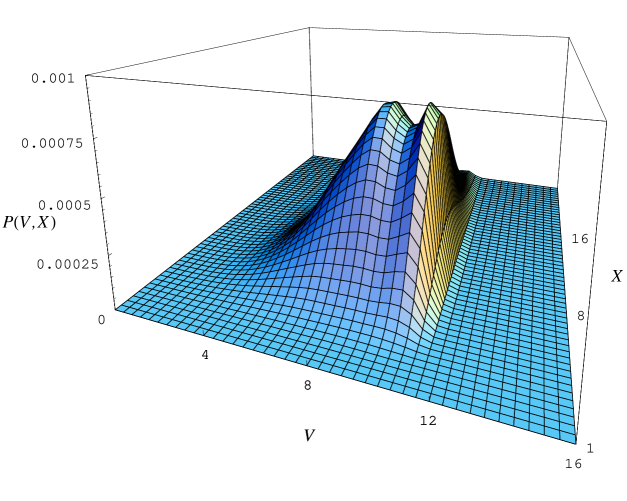
Figure 1: Probability density of headway $X$ and car velocity $V$ averaged over a group of 5 cars for $a=4$, $p_{2}/p_{0}=0.055$, $\mu=0.1$, and $v_{\rm max}=12$.

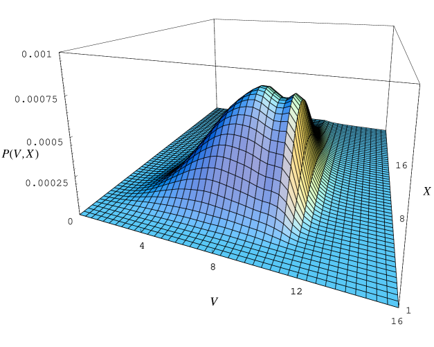
Figure 2: Probability density of headway $X$ and car velocity $V$ averaged over groups of 5 cars for $a=4$, $p_{2}/p_{0}=0.055$, $\mu=0.1$, with 70 % of cars of $v_{\rm max}=12$ and 30 % of $v_{\rm max}=20$.

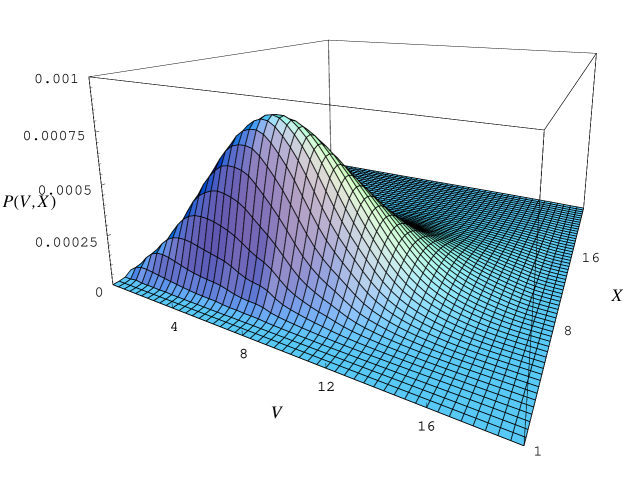
Figure 3: Probability density of headway $X$ and car velocity $V$ averaged over groups of 5 cars for $a=4$, $p_{2}/p_{0}=0.055$, $\mu=0.1$, with 2 % of cars of $v_{\rm max}=12$ and 98 % of $v_{\rm max}=20$.

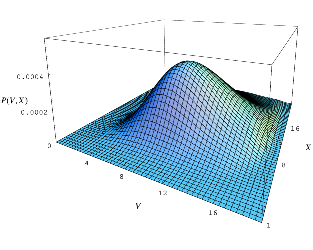
Figure 4: Probability density of headway $X$ and car velocity $V$ averaged over a group of 5 cars for $a=4$, $p_{2}/p_{0}=0.055$, $\mu=0.1$, with 100 % of cars of $v_{\rm max}=20$.

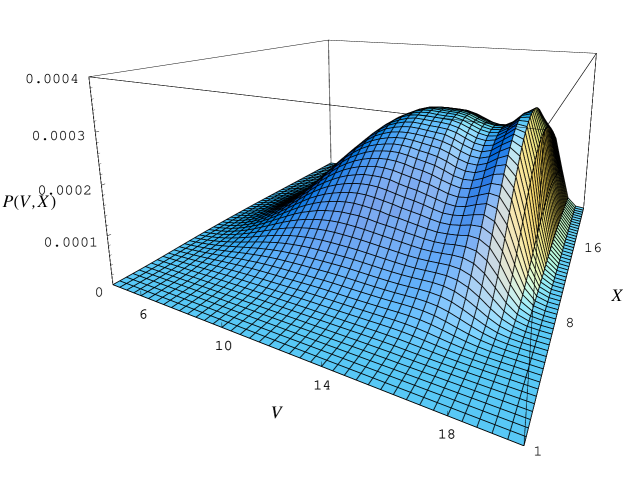
Figure 5: Probability density of headway $X$ and car velocity $V$ averaged over a group of 5 cars for $a=4$, $p_{2}/p_{0}=0.033$, $\mu=0.07$, with 100 % of cars of $v_{\rm max}=20$.

If all the cars have the smaller maximum velocity, $v_{\rm max}=12$, $p_{2}/p_{0}=0.055$, and $\mu=0.1$, the probability of velocity has two maxima practically of the same height (Fig. 1). Changing these two parameters, the relative heights of the peaks change, and eventually one of them disappears, i.e., a first order phase transition is observed in the system. This phase transition is also driven by ratio of slow and fast cars ($v_{\rm max}=20$) as seen from Fig. 2 where the increase of concentration of fast cars to 30 % causes an increase of the small velocity peak with respect to the high velocity one. Further addition of the fast cars makes the system even slower and denser (Fig. 3). Only total disappearance of slow cars causes an abrupt increase of mean velocity and distances between the vehicles. Nevertheless, the flow is not free, because of large value of the parameter $p_{2}/p_{0}$ the system is in the congested phase (Fig. 4), with the most probable velocity much smaller than $v_{\rm opt}$. For small values of the velocity spread $p_{2}/p_{0}$, potential $\mu$, and large deceleration rate, the car flow freely, and the probability diagram consists of a peak at $v_{\rm opt}$, narrow in $V$-direction and wide in $X$-direction.

For the fast cars with maximum velocity $v_{\rm max}=20$, the first order phase transition takes place at $p_{2}/p_{0}=0.033$, $\mu=0.07$ (Fig. 5). Now, addition of few slow cars, in distinction to the previous case, does not change the relative height of the two maxima, but totally destroys the probability diagram, and a wide peak in $V$-direction and narrow in $X$-direction is formed. (The probability diagram is similar to that in Fig. 2.) Density is higher and velocity lower than of the system consisting only of slow cars ($v_{\rm max}=12$).

As the cars cannot overtake each other, the most serious and instantaneous impact has a small admixture of cars with inferior properties to a free flowing pure system. On the other hand, addition of faster cars to a system of slow ones does not increase the mean velocity as well, but now the deterioration of the traffic flow is gradual.

If the braking abilities of the cars are poor, they form platoons of vehicles with the same, low velocity. The density of cars in the platoons is not small, and is varying in a large interval. In Fig. 6, the deceleration rate $a$ is 0.5 instead of $a=4$ of previous cases. $p_{2}/p_{1}$ is 0.1, potential $\mu=0.12$, and the maximum velocity $v_{\rm max}=20$. The presence of platoons is manifested by probability density maxima at integer values of the velocity.

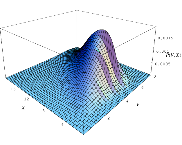
Figure 6: Probability density of headway $X$ and car velocity $V$ averaged over a group of 5 cars for $v_{\rm max}=20$, $p_{2}/p_{0}=0.1$, $\mu=0.12$, with 100 % of cars of $a=0.5$.

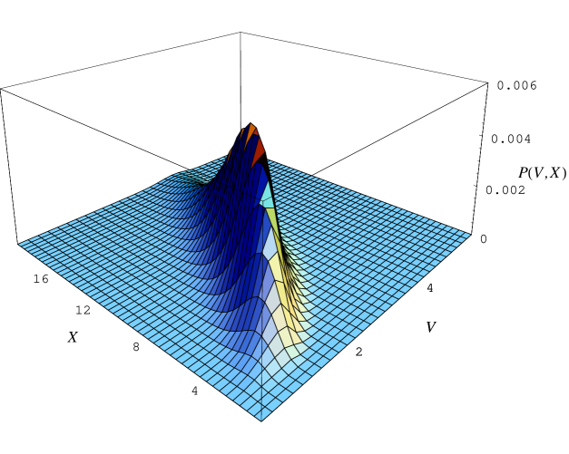
Figure 7: Probability density of headway $X$ and car velocity $V$ averaged over groups 5 indistinguishable cars for $v_{\rm max}=20$, $p_{2}/p_{0}=0.1$, $\mu=0.12$, with 90 % of cars of $a=0.5$ and 10 % of $a=4$.

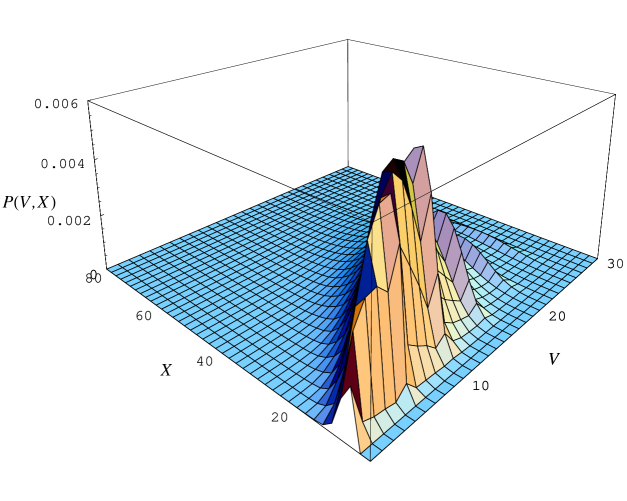
Figure 8: Probability density of headway $X$ and car velocity $V$ averaged over groups of 5 distinguishable cars for $v_{\rm max}=20$, $p_{2}/p_{0}=0.1$, $\mu=0.12$, with 90 % of cars of $a=0.5$ and 10 % of $a=4$.

If few cars with good brakes $(a=4)$ are added, and the drivers are not able to distinguish the quality of the car ahead, they should be more careful and decrease their velocity to, approximately, one half. The drivers of the cars with poor brakes have to assume that all the cars have effective brakes and to increase the headways. The platoons disappear, and the increase of the mean velocity with the mean distance between cars is slow (Fig. 7).

A different situation appears if the quality of the brakes of the preceding car is known to the driver. The cars with good brakes (type 1) may drive very closely to the cars with poor brakes (type 2). As the ratio of cars with good breaks is only 10% in Fig. 8, the cars with poor brakes drive mostly behind the cars of the same kind, the drivers know that, and formation of platoons is not hampered by the type 1 cars. All the cars move slowly so that also the distance between two cars with poor brakes is small, and the system is dense. Only the headway between type 1 and type 2 car is the same as all the headways in the previous case.

For the same parameters, but $a=4$, the cars move practically freely with only a small arm of slow vehicles (Fig. 9). This picture is destroyed by a small admixture (10%) of cars with poor brakes (Fig. 10). These cars should drive cautiously being surrounded by cars with good brakes which are able to stop immediately. They form very slow, dense platoons as at low velocity they are able to react effectively to slow cars in front of them. As in the front of cars with ineffective brakes there are practically always cars with good brakes, the possible knowledge of the type of the preceding car plays no role, and the diagram for $P(V,X)$ remains the same for both above-mentioned cases.

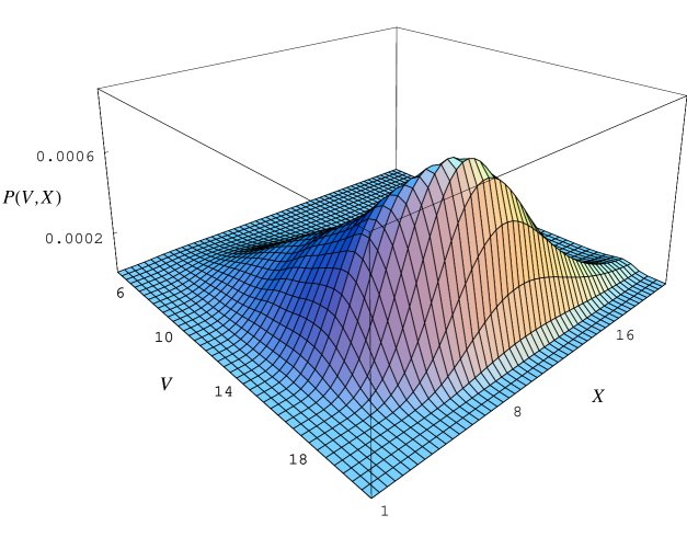
Figure 9: Probability density of headway $X$ and car velocity $V$ averaged over a group of 5 cars for $v_{\rm max}=20$, $p_{2}/p_{0}=0.1$, $\mu=0.12$, with 100 % of cars of $a=4$.

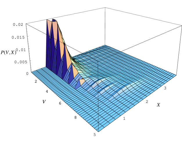
Figure 10: Probability density of headway $X$ and car velocity $V$ averaged over groups of 5 cars for $v_{\rm max}=20$, $p_{2}/p_{0}=0.1$, $\mu=0.12$, with 10 % of cars of $a=0.5$, 90 % of $a=4$.

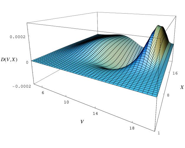
Figure 11: Difference of probability densities (7) of correlated and uncorrelated group of 5 cars for the same parameters as in figure 5.

All the peaks corresponding to free and congested flow or formation of platoons result from correlations between the cars. It is seen, e.g., in Fig. 11, where the difference between the probability density $D(V,X)$ of correlated and uncorrelated group of 5 cars, which $P(V,X)$ is in Fig. 5, is shown. The probability density of a group of uncorrelated cars always displays only a single peak without any internal structure.

4 Discussion

Deriving canonical distribution of an equilibrium gas of classical particles in statistical mechanics, all the velocities and positions of the particles are assumed to be equally probable, and a condition of given total mean energy is imposed on the system. (In grandcanonical distribution a condition for number of particles is added.) In our approach to the gas of cars all their relative positions are equally probable as well, but conditional probabilities of their velocities are given by behaviour of drivers. Instead of the condition on total energy, equality condition of mean velocities of all cars and a condition on the mean total length of the system are imposed. Now, the probability of a state has not a simple form of an exponential of the Hamiltonian like in the case of physical systems. In principle, it can be rewritten into such a form, but now the quantities appearing in the exponential are not conserved in an isolated system, what is the case in a gas of classical particles in physics. That is why it is not possible to introduce an effective energy or Hamiltonian in our system of cars, i.e., our approach differs from that of thermodynamical traffic gas [12] where interactions between cars and Hamiltonian of the system is introduced. Nevertheless, the results are similar but the velocity distribution of cars is not Gaussian.

Our method is, to some extent, similar to a mean-field and cluster approximation [8, 9, 10] looking for analytical solution of master equation corresponding to Nagel-Schreckenberg probabilistic cellular automaton model. Our choice of variables, velocities and headways, corresponds to that in the car oriented mean field theory [11], where the central role plays the probability $D_{n}(v)$ identical to our $P(v_{i-1},x_{i-1,i})$. In the above-mentioned approaches an approximate solution of master equations were found. In the present paper the solution is obtained by exact minimization of the entropy of the system.

Our results are consistent with a number of other approaches, based on kinetic or dynamical decripton of cars, and experimental observations of single line traffic [6, 13, 14]. It seems that systems of cars behave like many-particle physical systems or small parts of them, which, on microsopic level, are ruled by Newton or kinetic equations and, in equilibrium, are practically always described by canonical distribution derived from the principle of maximum entropy.

References

- [1] Nagel, K. and Schreckenberg, M., J. Phys. I (France) 2, 2221 (1992).
- [2] Maerivoet, S. and De Moor, B., Phys. Rep. 419, 1 (2005).
- [3] Chowdhury, D., Santen, L. and Schadschneider, A., Physics Reports 329, 199 (2000).
- [4] Šurda, A., J. Stat. Mech., P04017 (2008).
- [5] Herman, R. and Gardels, K., Sci. Am. 209, 35 (1963).
- [6] Kerner, B. S., Klenov, S. L., Hiller, A. and Rehborn, H., Phys. Rev. E 73, 046107 (2006).
- [7] Derrida, B., Phys. Rep. 301, 65 (1998).
- [8] Schadschneider, A., Physica A 313, 153 (2002).
- [9] Schadschneider, A. and Schreckenberg, M., J. Phys. A 26, L679 (1993).
- [10] Schreckenberg, M., Schadschneider, A., Nagel, K. and Ito, N., Phys. Rev. E 51, 2339 (1995).
- [11] Schadschneider, A. and Schreckenberg, M., J. Phys. A 30, L69 (1997).
- [12] Krbálek, M. J. Phys. A: Math. Theor. 40, 5813 (2007).
- [13] Wolf, D. E., Schreckenberg, M. and Bachem, A. (eds) 1996, Traffic and Granular Flow (Singapore, World Scientific); Helbing, D., Herrmann, H. J., Schreckenberg, M. and Wolf, D. E. (eds) 2000, Traffic and Granular Flow 99 (Berlin, Springer); Fukui, M., Sugiyama, Y., Schreckenberg, M. and Wolf, D. E. (eds) 2003, Traffic and Granular Flow 01 (Heidelberg, Springer); Hoogendoorn, S. P., Bovy, P. H. L., Schreckenberg, M. and Wolf, D. E. (eds) 2005, Traffic and Granular Flow 03 (Springer, Heidelberg)
- [14] Helbing, D., Rev. Mod. Phys. 73 1067 (2001).