Missing data in a stochastic Dollo model for cognate data, and its application to the dating of Proto-Indo-European

Abstract

Nicholls and Gray (2008) describe a phylogenetic model for trait data. They use their model to estimate branching times on Indo-European language trees from lexical data. Alekseyenko et al. (2008) extended the model and give applications in genetics. In this paper we extend the inference to handle data missing at random. When trait data are gathered, traits are thinned in a way that depends on both the trait and missing-data content. Nicholls and Gray (2008) treat missing records as absent traits. Hittite has 12% missing trait records. Its age is poorly predicted in their cross-validation. Our prediction is consistent with the historical record. Nicholls and Gray (2008) dropped seven languages with too much missing data. We fit all twenty four languages in the lexical data of Ringe et al. (2002). In order to model spatial-temporal rate heterogeneity we add a catastrophe process to the model. When a language passes through a catastrophe, many traits change at the same time. We fit the full model in a Bayesian setting, via MCMC. We validate our fit using Bayes factors to test known age constraints. We reject three of thirty historically attested constraints. Our main result is a unimodel posterior distribution for the age of Proto-indo-European centered at 8400 years BP with 95% HPD equal 7100-9800 years BP.

The Indo-European languages descend from a common ancestor called Proto-Indo-European. Lexical data show the patterns of relatedness among Indo-European languages. These data are “cognacy classes”: a pair of words in the same class descend, through a process of sound change, from a common ancestor. For example, English sea and German See are cognate to one another, but not to the French mer. Gray and Atkinson (2003) coded data of this kind in a matrix in which rows correspond to languages and columns to distinct cognacy classes, and entries are zero or one as the language possessed or lacked a term in the column class. They analysed these data using phylogenetic algorithms similar to those used for genetic data. Our analysis has the same objectives, but we fit a model designed for lexical trait data. We work with data compiled by Ringe et al. (2002), recording the distribution of some 872 distinct cognacy classes in twenty four modern and ancient Indo-European languages. In section 7, we give estimates for the unknown topology and branching times of the phylogeny of the core vocabulary of these languages.

Nicholls and Gray (2008) analyse the same data using a closely related stochastic Dollo-model for binary trait evolution. However, those authors were unable to deal with missing trait records. Missing data arise when we are unable to answer the question “does language X possess a cognate in cognacy class Y?”. Nicholls and Gray (2008) dropped seven languages which had many missing entries, and treated missing trait records in the remainder as absent traits. This is unsatisfactory. However, it is not straightforward to give a model-based integration of missing data for the trait evolution model of Nicholls and Gray (2008). In this paper we integrate the missing trait data, and this technical advance allows us to fit all twenty four of the languages in the original data. The binary trait model of Nicholls and Gray (2008), has been extended by Alekseyenko et al. (2008) to mutliple-level traits, and is finding applications in biology. A proper treatment of missing data will be of use in other applications.

We are specifically interested in phylogenetic dating. Because we are working with lexical, and not syntactic data, it is the age of the branching of the core vocabulary of Proto-Indo-European that we estimate. This is a controversial matter. Workers in historical linguistics have evidence from linguistic paleontology that the most recent common ancestor of all known Indo-European languages branched no earlier than about 6000–6500 years Before the Present (BP) (Mallory, 1989). For a recent review of the argument from linguistic paleontology, and a criticism of phylogenetic dating, see Garrett (2006) and McMahon and McMahon (2005). An alternative hypothesis suggests that the spread began around 8500 BP when the Anatolians mastered farming (Renfrew, 1987) in the early neolithic. Recent efforts to apply quantitative phylogenetic methods to dating Proto-Indo-European give a time depth of 8000 to 9500 years BP (Nicholls and Gray, 2008; Gray and Atkinson, 2003), supporting the link to farming. In this work we obtain a unimodal posterior distribution for the age of Proto-Indo-European centered at 8400 years BP with 95% HPD equal 7100-9800 years BP

One point of view is that the argument from linguistic paleontology is correct, and the phylogenetic dates are incorrect, due to rate heterogeneity, or some other model failing. In this respect we advance the search started in Nicholls and Gray (2008) for a model mispecification which might explain the 20% difference the central age estimates from our fitting, and the status quo. The difference is large enough that we are hopeful of finding a single coherent error, if any such error exists. Accounting now for missing data, we are able to publish a much wider cross-validation test (up from 10 to 30 tested calibrations). Also, we fit a model for explicit rate heterogeneity in time and space. In view of the spatial-temporal homogeneity we find here and in other data, the case for the earlier date seems now fairly strong. The most probable alternative seems to be a step change in the rate of lexical diversification acting in a coordinated fashion across the Indo-European territory some 3000 to 5000 years ago.

In Sections 1 and 2.1 we describe the data and specify a subjective prior for the phylogeny of vocabularies. In sections 2.2 and 3, we give a generative model for the data and the corresponding likelihood. We include, in Section 3, a recursive algorithm which makes the sum over missing data tractable. In sections 4 and 5 we give the posterior distribution on tree and parameter space, and briefly describe our MCMC sampler. In section 6, we discuss likely model mispecification scenarios, test for robustness by fitting synthetic data simulated under such conditions, and cross-validate our predictions. We fit the model to a data set of Indo-European languages in section 7. This paper has a supplement giving an analysis of a second data set, collected by Dyen et al. (1997).

Phylogenetic methods have been used to make inference for tree (Ringe et al., 2002) and network structure (McMahon and McMahon, 2005) in Historical Linguistics. Warnow et al. (2004) write down a more realistic model for the diversification of vocabulary, accounting for word-borrowing between languages (so that their history need not be tree-like) but there is to date no fitting.

1 Description of the data

The data group words from 328 meaning categories and 24 Indo-European languages into 872 homology classes. The data were collected and coded by Ringe et al. (2002). Meaning categories cover the “core” vocabulary and are assumed relevant to all languages in the study. Two words of closely similar meaning, descended from a common ancestor but subject to variation in phonology, are cognate terms. A cognacy class is a homology class of words all belonging to a single meaning category. For example, for the meaning “head", the Italian testa and the French tête belong to the same cognacy class, while the English head and the Swedish huvud belong to another cognacy class. An element of a cognacy class is thus a word in a particular language, a sound-meaning pair. These elements are called cognates. The vocabulary of a single language is represented as a set of distinct cognates. In our analysis a cognate has just two properties: its language and its cognacy class. If there are $N$ distinct cognacy classes in data for $L$ languages, then the $a$’th class $M_{a}\subseteq\{1,2,...,L\}$ is a list of the indices of languages which possess a cognate in that class. The data are coded as a binary matrix $D$. A row corresponds to a language and a column to a cognacy class, so that $D_{i,a}=1$ if the $a$’th cognacy class has an instance in the $i$’th language, and $D_{i,a}=0$ otherwise. See Table 1 for an example. This coding allows a language to have several words for one meaning (such as Old High German stirbit and touwit for ”he dies", an instance of polymorphism), or no word at all. Missing matrix elements arise because the reconstructed vocabularies of some ancient languages are incomplete. If we are unable to answer the question “does language $i$ possess a cognate in cognacy class $a$” then we set $D_{i,a}=?$.

We need notation for both matrix and set representations with missing data. Denote by $B_{a}$ column $a$ of $L\times N$ matrix $B$. For $a=1,2,...,N$ let ${\cal D}_{a}$ be the set of all column vectors $d^{*}$ allowed by the data $D_{a}$ in column $a$ of $D$,

$${\cal D}_{a}=\left\{d^{*}\in\{0,1\}^{L}:D_{i,a}\in\{0,1\}\Rightarrow d^{*}_{a}=D_{i,a},\ i=1,2,...,L\right\}.$$

For $d^{*}\in{\cal D}_{a}$ let $m(d^{*})=\{i:d^{*}_{i}=1\}$. Denote by $\Omega_{a}$ the set of cognacy classes consistent with the data $D_{a}$, so that

$$\Omega_{a}=\{\omega\subseteq\{1,2,\ldots,N\}:\omega=m(d^{*}),d^{*}\in{\cal D}_{a}\}.$$

The data $D$ are then equivalently $\Omega=(\Omega_{1},\Omega_{2},...,\Omega_{N})$. The $\Omega_{a}$-notation generalizes the $M_{a}$-notation to handle missing data. It is illustrated in Table 1.

$\begin{array}[]{c@{\hspace{.3in}}c}\begin{tabular}[]{|>{\bfseries}c|>{\itshape}c|}\hline\cr Old English&stierf\th\\ \hline\cr Old High German&stirbit, touwit\\ \hline\cr Avestan&miriiete\\ \hline\cr Old Church Slavonic&um\u{\i}ret\u{u}\\ \hline\cr Latin&moritur\\ \hline\cr Oscan&?\\ \hline\cr\end{tabular}\hfil\hskip 21.68121pt&\begin{tabular}[]{|>{\bfseries}c|ccc|}\hline\cr Old English&1&0&0\\ \hline\cr Old High German&1&1&0\\ \hline\cr Avestan&0&0&1\\ \hline\cr Old Church Slavonic&0&0&1\\ \hline\cr Latin&0&0&1\\ \hline\cr Oscan&?&?&?\\ \hline\cr\end{tabular}\\ \hfil\hskip 21.68121pt\\ (a)\hfil\hskip 21.68121pt&(b)\\ \hfil\hskip 21.68121pt\\ \end{array}$

Table 1: An example of data coding: (a), the word “he dies” in six Indo-European languages; (b), the coding of this data as a binary matrix with ?’s for missing data. In the notation of Section 1, the first column in (b) is a cognacy class $M_{\mbox{dies}}\in\Omega_{\mbox{dies}}$ with $\Omega_{\mbox{dies}}=\{\{\mbox{Old English, Old High German}\},\ \{\mbox{Old English, Old High German, Oscan}\}\}$

Ringe et al. (2002) list twenty four mostly ancient languages. For eleven of these languages (Latin, Modern Latvian, Old Norse…), all the matrix entries are recorded. For the rest, the proportion of missing entries varies between 1% (for Old Irish) and 91% (for Lycian, an ancient language of Anatolia). Note that data are usually missing in small blocks corresponding to the cognacy classes for a given meaning category, as in Table 1. We do not model this aspect of the missing data. This is related to the model-error Nicholls and Gray (2008) call ‘the empty-field approximation’, under which cognacy classes in the same meaning category are assumed to evolve independently.

For these Indo-European phylogenies, the topology of some subtrees are known from historical records. We have lower and upper bounds for the age of the root node of some subtrees. For example, the Slavic languages are known to form a subtree, and the most recent common ancestor of the Slavic languages in the data is known to be at least 1300 years old. In this way internal nodes of the phylogeny are constrained. We have age bounds for leaf nodes as well, since we are told when the vocabulary of the ancient languages in these data was in use. We combine these calibration constraints with the cognacy class data in section 2.1. Jumping ahead to our results, Figure 5 is a sample from the posterior distribution we find for phylogenies. Calibration constraints are represented by the black bars across nodes in this tree.

2 Models

We specify a subjective prior for phylogenies, representing a state of knowledge of interest to us. The model we give for the diversification of vocabulary in Section 2.2 is, in contrast, generative. We model the diversification of vocabulary as a branching process of sets of cognates, evolving on the phylogeny. Leaves are labeled by languages and a branch represents the ancestral lineage of a vocabulary.

2.1 Prior distribution on trees

The material in this subsection follows Nicholls and Gray (2008). We consider a rooted binary tree $g$ with $2L$ nodes: $L$ leaves, $L-2$ internal nodes, a root node $r=2L-1$ and an Adam node $A=2L$, which is linked to $r$ by a edge of infinite length. Each node $i=1,2,...,2L$ is assigned an age $t_{i}$ and $t=(t_{1},t_{2},...,t_{A})$; the units of age are years before the present; for the Adam node, $t_{A}=+\infty$. The edge between parent node $j$ and child node $i$ is a directed branch $\langle i,j\rangle$ of the phylogeny, with the orderings $i<j$ and $t_{i}<t_{j}$. Let $E$ be the set of all edges, including the edge $\langle r,A\rangle$, let $V$ be the set of all nodes and $V_{L}=\{1,2,...,L\}$ the set of all leaf nodes. Our base tree space $\Gamma$ is the set of all rooted directed binary trees $g=(E,V,t)$, with distinguishable leaves and, for $i=1,2,...,2L$, node ages $t_{i}>0$ assigned so that the directed path from a leaf $i\in V_{L}$ to node $A$ passes through nodes of strictly increasing age. With this numbering convention, $(E,V)$ is called the ordered history of a rooted directed binary tree.

We allow for $C$ calibration constraints on tree-topology and selected node ages. These are described at the end of Section 1. Each such constraint $c$ allows trees in just some subspace $\Gamma^{(c)}\subset\Gamma$ of tree space. We add to these constraints an upper bound on the root time at some age $T>0$, and set $\Gamma^{(0)}=\{(E,V,t)\in\Gamma:t_{r}\leq T\}$. The space of calibrated phylogenies with catastrophes is then

$$\Gamma^{C}=\bigcap_{c=0}^{C}\Gamma^{(c)}.$$

The root age is a sensitive statistic in this inference. A prior distribution on trees, with the property that the marginal distribution of the root age is uniform over a fixed prior range $t_{L}\leq t_{r}\leq T$, is of interest. For node $i\in V$, let $t^{+}_{i}=\sup_{g\in\Gamma^{C}}t_{i}$ and $t^{-}_{i}=\inf_{g\in\Gamma^{C}}t_{i}$ be the greatest and least admissible ages for node $i$, and let $S=\{i\in V:t^{+}_{i}=T\}$, so that $S$ is the set of nodes having ages not bounded above by a calibration (there are 12 such nodes in Figure (5)). Nicholls and Gray (2008) show that, before calibration (when $C=0$) and for tree spaces in which the leaves have fixed equal ages, the prior probability distribution with density

$$f_{G}(g|T)\propto\prod_{i\in S}(t_{r}-t^{-}_{i})^{-1}$$

gives a marginal density for $t_{r}$ which is exactly uniform in $t_{L}<t_{r}<T$. Nicholls and Gray (2008) do not comment on the distribution determined by $f_{G}$ over tree topologies. The prior $f_{G}$ has in this case ($C=0$) a uniform marginal distribution on ordered histories exactly equal to the corresponding distribution for the Yule model. This is not uniform, but favors balanced leaf-labeled topologies. For $C>0$, and on catastrophe-free tree spaces in which leaf ages are constrained by prior knowledge to lie in an interval only, Nicholls and Gray (2008) argue from simulation studies that this prior gives a reasonably flat marginal distribution for $t_{r}$ if in addition $T\gg\max_{i\in V\setminus S}t_{i}^{+}$ (the greatest upper bound among the calibration constraints is not too close to the upper bound on the root age). We give a sample from the prior in the Supplementary Material; the prior does not represent any reasonable prior belief before about 4500 BP, but this is immaterial as the likelihood rules these values out (an instance of an application of the principle of sufficient reason).

2.2 Diversification of cognacy classes

In this subsection we extend the stochastic Dollo model of Nicholls and Gray (2008) to incorporate rate heterogeneity in time and space, via a catastrophe process.

Consider the evolution of cognates down the ancestral lineage of the vocabulary of a single language. An example is given in Figure 1. A new cognacy class is born when its first cognate is born. This new word is not cognate with other words in the modeled process. Loan words from outside the core meaning categories of any language in the study, or from a language outside the study, may be good for word birth without violating this condition. A cognate dies in a particular vocabulary when it ceases to be used for the meaning common to its cognacy class: its meaning may change, or it may fall out of use.

Cognates evolving in a single language ($ie$ down a single branch of a language phylogeny) are born independently at rate $\lambda$, die independently at per capita rate $\mu$, and are subject to point-like catastrophes, which they encounter at rate $\rho$ along a branch. At a catastrophe, each cognate dies independently with probability $\kappa$, and a Poisson number of cognates with mean $\nu$ are born. At a branching event of the phylogeny, the set of cognates representing the branching vocabulary is copied into each of the daughter languages. See Figure 1.

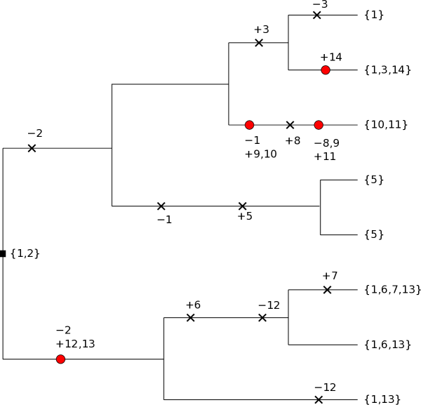
Figure 1: Description of the model: births and deaths of traits are marked. The dots correspond to catastrophes, at which multiple births and deaths may occur simultaneously. The cognate sets this generates at leaves are shown on the right. Calendar time flows from left to right and the age variables $t_{i}$ in the text increase from right to left.

The process we have described is not reversible, and this greatly complicates the analysis. It seems acceptable, from a data-modeling perspective, to impose the condition $\nu=\kappa\lambda/\mu$, which is necessary and sufficient for reversibility (see Supplementary Material for a proof). Under this condition, adding a catastrophe to an edge is equivalent to lengthening that edge by $T_{C}(\kappa,\mu)=-\log(1-\kappa)/\mu$ years. This follows because the number of cognates generated by the anagenic part of the process in an interval of length $T_{C}$ is Poisson distributed with mean $\frac{\lambda}{\mu}(1-e^{-\mu T_{C}})$ equal to $\kappa\lambda/\mu$, and the probability that a cognate entering an interval of length $T_{C}$ dies during that interval is $1-e^{-\mu T_{C}}$, which equals $\kappa$.

Because a catastrophe simply extends its edge by a block of virtual time, the likelihood depends only on the number of catastrophes on an edge, and not their location in time. Let $k_{i}$ be the number of catastrophes on edge $\langle i,j\rangle$, and $k=(k_{1},\ldots,k_{2L-2})$ be the catastrophe state vector. We record no catastrophes on the $\langle R,A\rangle$ edge (its length is already infinite). The tree $g=(V,E,t,k)$ is specified by its topology, node ages and catastrophe state. Calibrated tree space extended for catastrophes is

$$\Gamma^{C}_{K}=\{(V,E,t,k):(V,E,t)\in\Gamma^{C},k\in\mathbb{N}_{0}^{2L-2}\}.$$

We drop the catastrophe process from the calculation in Section 3. It is straightforward to restore it, and we do this in the expression for the posterior distribution in Section 4.

2.3 The registration process

Let ${\bf D}^{*}$ denote a notional full random binary data matrix, representing the outcome of the diversification process of Section 2.2. The number of columns in ${\bf D}^{*}$ is random, and equal to $N^{*}$. For the realization depicted in Figure 1, ${\bf D^{*}}=D^{*}$ with $D^{*}$ displayed in Figure 2.

[     D*     ]  [     I*     ]  [   D~       ]  [      I     ]  [      D     ]
10000000000000  11111111111111  10000000000000  1   111  1  11  1   000  0  00
10100000000001  01011111111111  ?0?00000000001  0   111  1  11  ?   000  0  01
00000000011000  10111001110110  0?000??001?00?  1   100  1  10  0   0??  1  0?
00001000000000  11111111111111  00001000000000  1   111  1  11  0   100  0  00
00001000000000  11110111111111  0000?000000000  1   011  1  11  0   ?00  0  00
10000110000010  10111111111111  1?000110000010  1   111  1  11  1   011  0  10
10000100000010  11111111111111  10000100000010  1   111  1  11  1   010  0  10
10000000000010  11111111111100  100000000000??  1   111  1  00  1   000  0  ??

Figure 2: Registration of the vocabulary realized in Figure 1 supposing a masking matrix $I^{*}$, as above. $D^{*}$ is the unobserved full data with a column for each cognacy class and a row for each language of Figure 1 (thus cognate 1 is present in rows 1,2,6,7 and 8); zeros in the masking matrix $I^{*}$ indicate missing matrix elements. Some cognacy classes are then thinned (in this example, the registration rule keeps cognacy classes with instances displayed in one or more language) to give the registered data $D$.

Note that $D^{*}$ has a column for each cognacy class present at the root node, or born below it, whether or not the cognacy class has any cognates represented in any leaf languages.

We call the random mapping of the unknown full representation ${\bf D}^{*}$ to the registered data $\bf D$, which is a random matrix with $N$ columns, the registration process. There are two stages to this process: the masking of matrix elements of the fully realised data $D^{*}$ with ?’s to form an intermediate data matrix $\tilde{D}$, and the selection of columns from $\tilde{D}$ to determine the realised data $D$.

Let ${\bf I}^{*}$ be a random $L\times N^{*}$ indicator matrix of independent Bernoulli random variables for observed elements. The zeros of $I^{*}$ mark matrix entries in $D^{*}$ which will be unobservable. For $i=1,2,...,L$ and given $a=1,2,...,N^{*}$, let $\xi_{i}=\Pr({\bf I}^{*}_{i,a}=1)$. The probability $\xi_{i}$ that we can answer the question, “does language $i$ possess a word in the $a$’th cognacy class?”, is assumed to be a function of the language index $i$ only. If we get an answer, it is assumed correct. Let $\xi=(\xi_{1},\ldots,\xi_{L})$ and denote by $I^{*}$ a realisation of ${\bf I}^{*}$. Denote by $\tilde{D}=\tilde{D}({D}^{*},{I}^{*})$ the masked version of the full random data matrix: if $I^{*}_{i,a}=1$ then $\tilde{D}_{i,a}=D^{*}_{i,a}$ and if $I^{*}_{i,a}=0$ then $\tilde{D}_{i,a}=?$.

Matrix columns may be missing too, so that $N\leq N^{*}$. We get missing columns even when there are no missing data. The matrix $\tilde{D}$ in Figure 2 includes some columns with only zeros and question marks, corresponding to cognacy classes which existed in the past but are observed in none of the leaf-languages from which the data were compiled. These cognacy classes are not included in the registered data. Denote by $R$ the registration rule ${\bf D}=R(\tilde{\bf D})$ mapping the full data to registered data.

Rule $R$ may thin additional column types. Let $Y$ and $Q$ be functions of the columns of $D^{*}$ and $I^{*}$ counting the visible 1’s and ?’s respectively,

$$Y({\bf D}^{*}_{a},{\bf I}^{*}_{a}) = \sum_{i=1}^{L}{\bf I}^{*}_{i,a}{\bf D}^{*}_{i,a},$$

$$Q({\bf I}^{*}_{a}) = \sum_{i=1}^{L}(1-{\bf I}^{*}_{i,a}).$$

Given $a=1,2,...,N^{*}$, let $Y_{a}=Y({\bf D}^{*}_{a},{\bf I}^{*}_{a})$ and $Q_{a}=Q({\bf I}^{*}_{a})$.

In Appendix A we give an efficient algorithm for computing the likelihood for rules formed by compounding the following elementary thinning operations:

1. $R_{1}(\tilde{D})=(\tilde{D}_{a}:Y_{a}>0)$ (discard classes with no instances at the leaves);

2. $R_{2}(\tilde{D})=(\tilde{D}_{a}:Y_{a}>1)$ (discard classes - singletons - observed at a single leaf);

3. $R_{3}(\tilde{D})=(\tilde{D}_{a}:Y_{a}<L)$ (discard classes which are observed at all leaves);

4. $R_{4}(\tilde{D})=(\tilde{D}_{a}:Y_{a}<L-1)$ (discard classes which are observed at all leaves or at all leaves but one);

5. $R_{5}(\tilde{D})=(\tilde{D}_{a}:Y_{a}+Q_{a}<L)$ (discard classes which are potentially present at all leaves);

6. $R_{6}(\tilde{D})=(\tilde{D}_{a}:Y_{a}+Q_{a}<L-1)$ (discard classes which are potentially present at all leaves or at all leaves but one).

We assume the chosen rule includes Condition (1). The rule $D=R(\tilde{D})$ with

$$R(\tilde{D})=R_{4}\circ R_{2}(\tilde{D})$$

collects “parsimony informative” cognacy classes. Ronquist et al. (2005) give the likelihood for the finite-sites trait evolution model of Lewis (2001) for registration rules like (1-6). In the example in Figure 2, and in Sections 6.2 and 7) we fit data registered with $R(\tilde{D})=R_{1}(\tilde{D})$.

The selection of columns is something we have in general no control over: the column selection rule simply describes what happened at registration. Results in the Supplementary Material for the Dyen et al. (1997) data use the rule $R(\tilde{D})=R_{2}(\tilde{D})$, since singleton columns were not included in that data. However, certain column types may include data which is hard to model well, and so we may choose to make further thinning using the other rules. Recursions for the other rules are given in an Appendix.

Column indices $a=1,2,...,N^{*}$ are exchangeable. It is convenient to renumber the columns of $D^{*}$, $I^{*}$ and $\tilde{D}$ after registration, so that $\tilde{D}_{a}=D_{a}$ and $I^{*}_{a}=I_{a}$ for $a=1,2,...,N$. The information needed to evaluate $Y_{a}$ and $Q_{a}$ is available in the column $D_{a}$ and set $\Omega_{a}$ representations. We write $Y(D_{a})=Y(\Omega_{a})=Y_{a}$ and $Q(D_{a})=Q(\Omega_{a})=Q_{a}$.

2.4 Point process of births for registered cognacy classes

Fix a catastrophe-free phylogeny $g\in\Gamma^{C}_{K}$, with $k=(0,0,...,0)$, and let an edge $\langle i,j\rangle$ and a time $\tau\in[t_{i},t_{j})$ be given. Denote by $[g]$ the set of all points $(\tau,i)$ on the phylogeny, including points $(\tau,r)$ with $\tau\geq t_{r}$ in the edge $\langle r,A\rangle$. The locations $z_{D}=\{z_{1},z_{2},...,z_{N}\}$ of the birth events of the $N$ registered cognacy classes are a realization of an inhomogeneous Poisson point process $Z_{D}$ on $[g]$. Let $Z\in[g]$ be the birth location of a generic (and possibly unregistered) cognacy class $M\subseteq\{1,2,...,L\}$, corresponding to a column of $\tilde{\bf D}$ with $Y$ observed $1$’s and $Q$ $?$’s, and let ${\cal E}_{Z}$ be the event that this class generates a column of the registered data. For the $a$’th cognacy class $M_{a}$, born at $Z_{a}$, this event is ${\cal E}_{Z_{a}}=\{{\bf D}_{a}=R(\tilde{\bf D}_{a})\}$ since $R(\tilde{\bf D}_{a})$ is empty for $\tilde{\bf D}_{a}$ a column dropped at registration.

Cognacy classes are born at constant rate on the branches of $g$, but are thinned by registration. However, conditional on the birth location $Z_{a}=z_{a}$, our modeling assumes that the outcome ${\cal E}_{Z_{a}}$ for the $a$’th cognacy class is decided independently of all events in all other cognacy classes. The point process $Z_{D}$ of birth locations of registered cognacy classes has intensity

$$\tilde{\lambda}(z)=\lambda\Pr({\cal E}_{Z}|g,\mu,\lambda,\xi,Z=z)$$

at $z\in[g]$ and probability density

$$f_{Z_{D}}(z_{D})=\frac{1}{N!}e^{-\Lambda([g])}\prod_{a=1}^{N}\tilde{\lambda}(z_{a})$$

with respect to the element of volume $dz_{D}=dz_{1}dz_{2}...dz_{N}$ in $[g]^{N}$, where

$$\Lambda([g]) = \int_{[g]}\tilde{\lambda}(z)dz$$

$$= \sum_{\langle i,j\rangle\in E}\int_{t_{i}}^{t_{j}}\tilde{\lambda}((\tau,i))d\tau.$$

The number $N$ of registered cognacy classes is $N\sim\mbox{Poisson}(\Lambda([g]))$.

3 Likelihood calculations

We give the likelihood for $g$, $\mu$, $\lambda$, $\kappa$, $\rho$ and $\xi$ given the data, along with an efficient algorithm to compute the sum over all missing data. The catastrophe process is left out, and reincorporated in the next section.

Since we only ever see registered data, the likelihood for $g,\lambda,\mu$ and $\xi$ is the probability $P[{\bf D}=D|g,\mu,\lambda,\xi,{\bf D}=R(\tilde{\bf D})]$, to get data $D$ given the parameters and conditional on the data having passed registration. We restore the birth locations (and so omit $\lambda$ from the conditioning), and factorize using the joint independence of $D_{a},a=1,2,...,N$ under the given conditions:

$$P[{\bf D}\!=\!D|g,\mu,\lambda,\xi,{\bf D}\!=\!R(\tilde{\bf D})] \!=\! \int f_{Z_{D}}(z_{D})P[{\bf D}\!=\!D|g,\mu,\xi,Z_{D}\!=\!z_{D},{\bf D}\!=\!R(\tilde{\bf D})]\,dz_{D},$$

$$\!=\! \frac{e^{-\Lambda([g])}}{N!}\prod_{a=1}^{N}\lambda\int_{[g]}\!\!P[{\cal E}_{Z_{a}}|g,\mu,\xi,Z_{a}\!=\!z_{a}]\ \!P[{\bf D}_{a}\!=\!D_{a}|g,\mu,\xi,Z_{a}\!=\!z_{a},{\cal E}_{Z_{a}}]\,dz_{a},$$

$$\!=\! \frac{e^{-\Lambda([g])}}{N!}\prod_{a=1}^{N}\lambda\int_{[g]}\!\!P[{\bf D}_{a}\!=\!D_{a}|g,\mu,\xi,Z_{a}\!=\!z_{a}]\,dz_{a}.$$

The last line follows because $P[{\cal E}_{Z_{a}}|{\bf D}_{a}=D_{a},...,Z_{a}=z_{a}]=1$ for $D_{a}$ a column of registered data: if the outcome of the birth at $z_{a}$ was the registerable data $D_{a}$ then the event ${\cal E}_{Z_{a}}$ certainly occurs. The likelihood depends on the awkward condition ${\bf D}=R(\tilde{\bf D})$ through the mean number $\lambda([g])$ of registered cognacy classes only, while $P[{\bf D}_{a}=D_{a}|g,\mu,\xi,Z_{a}=z_{a}]$ is the probability to realise the data vector $D_{a}$ in the unconditioned diversification/missing element process. The calculation has so far extended Nicholls and Gray (2008) to give the likelihood for a greater variety of column thinning rules. We now add the missing element component of the registration process.

We sum over possible values of the missing matrix elements in the registered data. Since $P[{\bf D}_{a}=D_{a}|g,\mu,\lambda,\xi,Z_{a}=z_{a}]$ is not conditioned on the requirement that the column $D_{a}$ gets registered, the entries of the corresponding column $I_{a}$ are determined by the unconditioned Bernoulli process, and we have

$$P[{\bf D}_{a}=D_{a}|g,\mu,\xi,Z_{a}=z_{a}] = \sum_{d^{*}\in{\cal D}_{a}}P[{\bf I}^{*}_{a},{\bf D}^{*}_{a}=d^{*}|g,\mu,\xi,Z_{a}=z_{a}]$$

$$= \prod_{i=1}^{L}\xi_{i}^{I_{i,a}}(1-\xi_{i})^{1-I_{i,a}}\sum_{d^{*}\in{\cal D}_{a}}P[{\bf D}^{*}_{a}=d^{*}|g,\mu,\xi,Z_{a}=z_{a}].$$

The likelihood is

$$P[{\bf D}=D|g,\mu,\lambda,\xi,{\bf D}=R(\tilde{\bf D})]=\frac{e^{-\Lambda([g])}}{N!}\prod_{a=1}^{N}(\prod_{i=1}^{L}\xi_{i}^{I_{i,a}}(1-\xi_{i})^{1-I_{i,a}})\lambda\int_{[g]}\sum_{\omega\in\Omega_{a}}P[M=\omega|g,\mu,\xi,Z=z_{a}]dz_{a},$$ (1)

where we have switched now from summing $d^{*}\in{\cal D}_{a}$ to the equivalent set representation $\omega\in\Omega_{a}$.

For the two integrated quantities in Equation (1) we have tractable recursive formulae. We are using a pruning procedure akin to Felsenstein (1981). We begin with $\Lambda([g])$.

We assume the registration rule includes at least Condition (1). It follows that a cognacy class born at $Z=(\tau,i)$ in $[g]$ must survive down to the node below, at $Z=(t_{i},i)$, in order to be registered, and so

$$P[{\cal E}_{Z}|Z=(\tau,i),g,\mu,\xi]=P[{\cal E}_{Z}|Z=(t_{i},i),g,\mu,\xi]e^{-\mu(\tau-t_{i})}.$$

We can substitute this into the expression for $\Lambda([g])$, and integrate, to get

$$\Lambda([g])=\frac{\lambda}{\mu}\sum_{\langle i,j\rangle\in E}P[{\cal E}_{Z}|Z=(t_{i},i),g,\mu,\xi]\left(1-e^{-\mu(t_{j}-t_{i})}\right).$$ (2)

Given a node $i$, let $V_{L}^{(i)}$ be the set of leaf nodes descended from $i$, including $i$ itself if $i$ is a leaf. Let $s_{i}=\mbox{card}(V_{L}^{(i)})$. Denote by $u_{i}^{(n)}=P[Y=n|Z=(t_{i},i),g,\mu,\xi]$ and $v_{i}^{(n)}=P[Y+Q=n|Z=(t_{i},i),g,\mu,\xi]$. We can compute $\Lambda$ for rules made up of combinations of Condition (1) with any combination of Conditions (2-6), from $u_{i}^{(0)}$, $u_{i}^{(1)}$, $u_{i}^{(s_{i}-1)}$, $u_{i}^{(s_{i})}$, $v_{i}^{(s_{i}-1)}$ and $v_{i}^{(s_{i})}$. For example,

$$P[{\cal E}_{Z}|Z=(t_{i},i),g,\mu,\xi]=\left\{\begin{array}[]{ll}1-u_{i}^{(0)}&R=R_{1},\\ 1-u_{i}^{(0)}-u_{i}^{(1)}&R=R_{2},\\ 1-u_{i}^{(0)}-u_{i}^{(1)}-u_{i}^{(L-1)}-u_{i}^{(L)}&R=R_{3}\circ R_{2}.\}\end{array}\right.$$ (3)

Notice that $u_{i}^{(n)}=0$ unless $s_{i}\geq n$, so for example $u_{i}^{(L)}$ is non-zero at $i$ the root node only. Since our main application is for data registered under Condition (1), we give, in the body of this paper, recursions for $u_{i}^{(0)}$ and $v_{i}^{(0)}$ only. See Appendix A for the recursions needed to evaluate the likelihood under rules involving Conditions (2-6).

For nodes $i$ and $j$, let $\delta_{i,j}=e^{-\mu(t_{j}-t_{i})}$. Consider a pair of edges $\langle c_{1},i\rangle$, $\langle c_{2},i\rangle$ in $E$.

$$u_{i}^{(0)} = \left((1-\delta_{i,c_{1}})+\delta_{i,c_{1}}u_{c_{1}}^{(0)}\right)\left((1-\delta_{i,c_{2}})+\delta_{i,c_{2}}u_{c_{2}}^{(0)}\right)$$ (4)

$$v_{i}^{(0)} = \left(\delta_{i,c_{1}}v_{c_{1}}^{(0)}+(1-\delta_{i,c_{1}})\prod_{j\in V_{L}^{c_{1}}}\xi_{j}\right)\left(\delta_{i,c_{2}}v_{c_{2}}^{(0)}+(1-\delta_{i,c_{2}})\prod_{j\in V_{L}^{c_{2}}}\xi_{j}\right)$$ (5)

The recursion is evaluated from the leaves $i\in V_{L}$, at which

$$u_{i}^{(0)} = 1-\xi_{i}$$ (6)

$$v_{i}^{(0)} = 0$$ (7)

We now give the equivalent recursions for $\lambda\int_{[g]}\sum_{\omega\in\Omega_{a}}P[M=\omega_{a}|Z=z_{a},g,\mu]\,dz_{a}$. Consider the set $m_{a}=\bigcap_{\omega\in\Omega_{a}}\omega$ of leaves known to have a cognate in the $a$th registered cognacy class. Let $E_{a}$ be the set of branches on the path from the most recent common ancestor of the leaves in $m_{a}$ up to the Adam-node $A$ above the root. Cognacy class $a$ must have been born on an edge in $E_{a}$. For $a=1,2,...,N$, class $M_{a}$ is non-empty and we can shift the birth location to the node below and convert the integral to a sum,

$$\lambda\int_{[g]}\sum_{\omega\in\Omega_{a}}P[M=\omega|Z=z_{a},g,\mu]\,dz_{a}=\frac{\lambda}{\mu}\sum_{\langle i,j\rangle\in E_{a}}\sum_{\omega\in\Omega_{a}}P[M=\omega|Z=(t_{i},i),g,\mu](1-\delta_{i,j}).$$

For each $a=1,2,...,N$ and $\omega\in\Omega_{a}$, let $\omega^{(i)}=\omega\cap V_{L}^{(i)}$ and

$$\Omega_{a}^{(i)}=\{\omega^{(i)}:\omega^{(i)}=\omega\cap V_{L}^{(i)},\omega\in\Omega_{a}\}$$

denote the set of all subsets $\omega^{(i)}$ of the leaves $V_{L}^{(i)}$ which are cognacy classes consistent with the data available for those leaves. Consider two child branches $\langle c_{1},i\rangle$ and $\langle c_{2},i\rangle$ at node $i$. Since $\Omega_{a}=\Omega_{a}^{(c_{1})}\times\Omega_{a}^{(c_{2})}$, and events are independent along the two branches,

$$\sum_{\omega\in\Omega_{a}}P[M=\omega|Z=(t_{i},i),g,\mu,\xi] = \sum_{\omega^{(c_{1})}\in\Omega_{a}^{(c_{1})}}P[M=\omega^{(c_{1})}|Z=(t_{i},c_{1}),g,\mu]$$

$$\times\sum_{\omega^{(c_{2})}\in\Omega_{a}^{(c_{2})}}P[M=\omega^{(c_{2})}|Z=(t_{i},c_{2}),g,\mu].$$

Having moved the birth event at $(t_{i},i)$ to $(t_{i},c_{1})$ and $(t_{i},c_{2})$ (off the node and onto its child edges) we now move the birth event at $(t_{i},c)$ to $(t_{c},c)$ (down an edge) as follows:

$$\sum_{\omega\in\Omega_{a}^{(c)}}P[M=\omega|Z=(t_{i},c),g,\mu]=$$

$$\left\{\begin{array}[]{ll}\delta_{i,c}\times\displaystyle\sum_{\omega\in\Omega_{a}^{(c)}}P[M=\omega|Z=(t_{c},c),g,\mu]&\text{ if }Y(\Omega_{a}^{(c)})\geq 1\\ (1-\delta_{i,c})+\delta_{i,c}\times\displaystyle\sum_{\omega\in\Omega_{a}^{(c)}}P[M=\omega|Z=(t_{c},c),g,\mu]&\text{ if }Y(\Omega_{a}^{(c)})=0\text{ and }Q(\Omega_{a}^{(c)})\geq 1\\ (1-\delta_{i,c})+\delta_{i,c}v_{c}^{(0)}&\text{ if }Y(\Omega_{a}^{(c)})+Q(\Omega_{a}^{(c)})=0\\ &\quad\text{(\emph{i.e.} }\Omega_{a}^{(c)}=\{\emptyset\}\text{)}\end{array}\right.$$

The recursion is evaluated from the leaves. If $c$ is a leaf, then

$$\ \sum_{\omega\in\Omega_{a}^{(c)}}P[M=\omega|Z=(t_{c},c),g,\mu]=\begin{cases}1&\text{ if }\Omega_{a}^{(c)}=\{\{c\},\emptyset\}\text{ or }\{\{c\}\}\text{ (\emph{i.e.} }D_{c,a}\in\{?,1\}\text{)}\\ 0&\text{ if }\Omega_{a}^{(c)}=\{\emptyset\}\text{ (\emph{i.e.} }D_{c,a}=0\text{)}.\end{cases}$$

In order to restore catastrophes to this calculation, and given $g\in\Gamma_{K}$, with $k_{i}$ catastrophes on edge $\langle i,j\rangle\in E$, replace $t_{j}-t_{i}$ with $t_{j}-t_{i}+k_{i}T_{C}(\kappa,\mu)$ throughout.

4 Posterior distribution

Our prior on the birth rate $\lambda$, death rate $\mu$ and catastrophe rate $\rho$ is $p(\lambda,\mu,\rho)\propto\frac{1}{\lambda\mu\rho}$ and we take a uniform prior over $[0,1]$ for the death probability at a catastrophe $\kappa$ and each missing data parameter $\xi_{i}$.

Substituting using equations (2)-(3) into equation (1) and multiplying by the prior $f_{G}(g|T)p(\lambda,\mu,\rho)$, we obtain the posterior distribution

$$p(g,\mu,\lambda,\kappa,\rho,\xi|{\bf D}=D)$$ (9)

$$= \frac{1}{N!}\left(\frac{\lambda}{\mu}\right)^{N}\exp\left(-\frac{\lambda}{\mu}\sum_{\langle i,j\rangle\in E}P[{\cal E}_{Z}|Z=(t_{i},i),g,\mu,\kappa,\xi](1-e^{-\mu(t_{j}-t_{i}+k_{i}T_{C})})\right)$$

$$\times\prod_{a=1}^{N}\left(\sum_{\langle i,j\rangle\in E_{a}}\sum_{\omega\in\Omega_{a}}P[M=\omega|Z=(t_{i},i),g,\mu](1-e^{-\mu(t_{j}-t_{i}+k_{i}T_{C})})\right)$$

$$\times\frac{1}{\mu\lambda\rho}f_{G}(g|T)\frac{e^{-\rho|g|}(\rho|g|)^{k_{T}}}{k_{T}!}\prod_{i=1}^{L}(1-\xi_{i})^{Q_{i}}\xi_{i}^{N-Q_{i}}$$

for parameters $\mu,\lambda,\kappa,\rho>0$, $0<\xi_{i}<1$ and trees $g\in\Gamma_{K}^{(C)}$.

The posterior is improper without bounds on $\rho$ since $k_{T}=0$ is allowed. We place very conservative bounds on $\rho$. Results are not sensitive to this choice. We can show that, for ’typical’ data sets $D$, and in particular the data analysed below, the posterior is then proper. Details of the relationship between cognate classes and calibration constraints play a role in the conditions for the posterior distribution to be proper.

5 Markov Chain Monte Carlo

We use Markov Chain Monte Carlo to sample the posterior distribution and estimate summary statistics. If the prior on the cognacy class birth rate parameter $\lambda$ has the conjugate form $\lambda^{u}\exp(-v\lambda)$ then the conditional distribution of $\lambda$ in the posterior distribution above has the form $\lambda^{N+u}\exp(-\lambda(X+v))$. We took the improper prior $u=-1$, $v=0$ for $\lambda$ and integrated. The MCMC state is then $x=((E,V,t,k),\mu,\kappa,\rho,\xi)$ and the target distribution $p(x|D)$ is the density obtained by integrating the density in Equation 9 over $\lambda$.

The MCMC sampler described in Nicholls and Gray (2008) has state $x=((E,V,t),\mu)$. We add to the $(E,V,t)$- and $\mu$-updates of Nicholls and Gray (2008) further MCMC updates acting on the catastrophe vector $k=(k_{1},...,k_{L-2})$, on the catastrophe parameters $\kappa,\rho$ and on $\xi$, the probability parameter for observable data-matrix elements. The catastrophe rate parameter $\rho$ is added to time-scaling updates in which subsets of parameters are simultaneously scaled by a common random factor $s$: if $\theta$ is a parameter in the scaled subset having units $[\mbox{time}]^{u}$, then $\theta\rightarrow s^{u}\theta$. The probability $0<\xi_{i}<1$ for an element of the registered data matrix to be observable is, for many leaf-languages, close to one, so we update those parameters by scaling $1-\xi_{i}$.

We incorporate updates adding and deleting catastrophes (the filled dots marked on the branches of Figure 1) plus an update which moves a catastrophe from an edge to a parent, child or sibling edge. For the addition and deletion of catastrophes, we do not need to use reversible jump Markov Chain Monte Carlo, as the state vector specifies the numbers, and not the locations, of catastrophes on edges.

We omit the details of these moves but give, as an example, the update that moves a catastrophe from an edge to a parent, child or sibling edge. Let $k_{T}=\sum_{i=1}^{L-2}k_{i}$ give the total number of catastrophes. Given a state $x=(g,\mu,\kappa,\rho,\xi)$ with $g=(V,E,t,k)$, we pick edge $\langle i,j\rangle\in E$ with probability $k_{i}/k_{T}$. Let $E_{\langle i,j\rangle}$ be the set of edges neighbouring edge $\langle i,j\rangle$ (child, sibling and parent edges, but excluding the edge $\langle R,A\rangle$) and let $q_{i}=\mbox{card}(E_{\langle i,j\rangle})$. We have in general $q_{i}=4$. However, for $i$ the index of a leaf node, $q_{i}=2$ (1 parent, 1 sibling, no children). If $j$ is the root and $i$ is non-leaf, then $q_{i}=3$ (1 sibling, 2 children) and if $j$ is the root and $i$ is a leaf we have $q_{i}=1$ (a sibling edge). Choose a neighbouring edge $\langle\tilde{i},\tilde{j}\rangle$ uniformly at random from $E_{\langle i,j\rangle}$ and move one catastrophe from $\langle i,j\rangle$ to $\langle\tilde{i},\tilde{j}\rangle$. The candidate state is $x^{\prime}=((V,E,t,k^{\prime}),\mu,\kappa,\rho)$, with $k_{i}^{\prime}=k_{i}-1$ and $k_{\tilde{i}}^{\prime}=k_{\tilde{i}}+1$ and $k^{\prime}_{j}=k_{j}$ for $j\neq i,\tilde{i}$. This move is accepted with probability

$$\alpha(x^{\prime}|x)=\min\left(1,\frac{q_{i}\,k_{\tilde{i}}^{\prime}\,p(x^{\prime}|D)}{q_{\tilde{i}}\,k_{i}\,p(x|D)}\right).$$

We assessed convergence with the asymptotic behaviour of the autocorrelation for the parameters $\mu$, $\kappa$, $\rho$ and $t_{R}$, as suggested by Geyer (1992). This method indicated that we could use runs of about 10 million samples; we also let the MCMC run for 100 million samples and checked that the computed statistics did not vary.

6 Validation

We made a number of tests using synthetic data. Fitting the model to synthetic data simulated according to the likelihood $P({\bf D}=D|g,\mu,\lambda,\rho,\kappa,\xi,{\bf D}=R(\tilde{\bf D}))$, (in-model data), shows us just how informative the data is for catastrophe placement, as well as making a debug-check on our implementation. We fit out-of-model data also. These are synthetic data simulated under likely model-violation scenarios, and are used to identify sources of systematic bias. We summarise results for synthetic data simulated using the parameter values we estimate in section 7 on the data. For in-model data we correctly reconstruct topology, root age and the number and position of catastrophes. Further details are given in the Supplementary Material.

6.1 Model mis-specification

Nicholls and Gray (2008) use out-of-model data representing un-modeled loan-words (called borrowing), rate-heterogeneity in time and space, rate heterogeneity across cognacy classes, and the empty-field approximation. They discuss also model mis-specification due to missing data and the incorrect identification of cognacy classes (in particular, a hazard for deeply rooted classes to be split). Rate-heterogeneity in time and space, and missing data are now part of the in-model analysis.

We synthesized out-of-model data with the borrowing model of Nicholls and Gray (2008), in order to see if un-modeled borrowing biased our results. For what Nicholls and Gray (2008) call low to moderate levels of borrowing, we were able to reconstruct true parameter values well. See the Supplementary Material for details. With high levels of borrowing, we under-estimate the root age and over-estimate rate parameters. However, unidentified loan words in the registered data do not generate model mispecification unless they are copies of cognates which occur in the observed meaning categories of languages ancestral to the leaf-languages. It is not plausible that unidentified borrowing of this kind is present at high levels.

We have not repeated the Nicholls and Gray (2008) out-of-model analysis of rate heterogeneity across cognacy classes.

In a real vocabulary, distinct cognacy classes that share a meaning category would not evolve independently. Also, a real language might be expected to a possess a word in each of the core meaning categories. This constrains the number of cognacy classes in each meaning category to be non-zero. Our model allows empty meaning categories. Nicholls and Gray (2008) find no substantial bias in a fit to out-of-model data respecting the constraint.

Our treatment of missing data introduces a new mis-specification. We modeled matrix elements as missing independently. However, we get missing data when we do not know the word used in a given language to cover a given meaning category. Matrix elements are as a consequence typically missing in blocks corresponding to all the cognacy classes for the given meaning. Because the ages of poorly reconstructed languages are well predicted in the cross-validation study below, we have not looked further at this issue.

6.2 Prediction tests for calibration

In the next section we estimate the age of a tree node (the root). In this sectio nwe test to see if the uncertainties we estimate are reliable.

The calibration data described in Section (1) fix the topologies and root ages of the subtrees marked with bars in Figure 5). We remove each calibration constraint in turn and use the data and the remaining constraints to estimate the age of the constrained node, and the probability for the constrained subtree topology. The topological constraints were all perfectly reconstructed. In twenty three of the twenty eight tests the constrained age interval overlaps the 95% HPD interval, as shown in the bottom half of Figure 3.

How good or bad are each of these predictions? Looking at the Hittite prediction in Figure 3, the large prediction uncertainty only just allows the calibration interval. Is this bad? We quantify the goodness-of-fit, for each calibration, using Bayes factors to replace $p$-values as indices of misfit. For each constraint $c=1,2,...,C$ we compute a Bayes factor measuring the support for the fully constrained model compared to a model with just the $c$’th constraint removed.

For $c=1,2,...,C$ let

$$\Gamma^{C-c}=\bigcap_{c^{\prime}=0\atop c^{\prime}\neq c}^{C}\Gamma^{(c^{\prime})}.$$

denote the enlarged tree space with the $c$’th constraint removed, and let $\Gamma^{C-c}_{K}$ be the enlarged tree space, extended to include catastrophes (as in Section (2.2)). For each constraint $c=1,2,...,C$ we make a model comparison between a common null model with all the constraints, $H_{0}:g\in\Gamma^{C}_{K}$, and an alternative model $H_{1}:g\in\Gamma^{C-c}_{K}$ with the constraint removed. The Bayes factor $B_{C,C-c}$ for the model comparison is the ratio of the posterior probabilities for these models with model prior $P(H_{0})=P(H_{1})$,

$$B_{-c} = \frac{P(D|g\in\Gamma^{C}_{K})}{P(D|g\in\Gamma^{C-c}_{K})}$$

$$= \frac{P(D|g\in\Gamma^{C}_{K}\cap\Gamma^{C-c}_{K})}{P(D|g\in\Gamma^{C-c}_{K})}$$

$$= \frac{P(g\in\Gamma^{C}_{K}|D,g\in\Gamma^{C-c}_{K})}{P(g\in\Gamma^{C}_{K}|g\in\Gamma^{C-c}_{K})}.$$

where the second line follows since $\Gamma^{C}_{K}\subset\Gamma^{C-c}_{K}$ and the third from the definition of the conditional probabilities. The numerator $P(g\in\Gamma^{C}_{K}|D,g\in\Gamma^{C-c}_{K})$ is the posterior probability for the $c$’th constraint to be satisfied given the data and the other constraints. The denominator, $P(g\in\Gamma^{C}_{K}|g\in\Gamma^{C}_{K})$, is the prior probability for the $c$’th constraint to be satisfied given the other constraints. We estimate these probabilities using simulation of the posterior and prior distributions with constraint $c$ removed. The Bayes factors are estimated with negligible uncertainty and $2\log(B_{C,C-c})$ is plotted for $c=1,2,...,C$ in the top half of Figure 3.

Strong evidence against a calibration is failure at prediction. Taking a Bayes factor exceeding 12 (that is, $2\log(B_{C,C-c})\gtrsim 5$ in Figure 3) as strong evidence against the constraint, following Raftery (1996), we have conflict for three of the thirty constraints: the ages of Old Irish and Avestan, and for the age of the Balto-Slav clade. As our analysis in Section 7 shows, there is a high posterior probability that a catastrophe event occurred on the branch between Old Irish and Welsh, and another between Old Persian and Avestan. The evidence for rate heterogeneity in rest of the tree is so slight, that when we try to predict these calibrations we are predicting atypical events.

Our missing-data analysis has helped here. The calibration interval for the Hittite vocabulary in these data is 3200–3700BP. A reconstruction of the age of Hittite which ignores missing data predicts 60–2010BP, well outside of the constraints. The 95% HPD interval for the age of Hittite in our model is 430–3250BP, which just overlaps the constraint. The Bayes factor gives odds less than 3:1 against, so the evidence against the constraint is ‘hardly worth mentioning’.

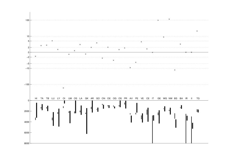
Figure 3: Reconstruction of known node ages: top, logarithm of Bayes factors $\log(B_{C,C-c})$ for $c=1,2,...,C$; bottom, thin lines show age constraints for different nodes, thick lines show 95% posterior HPD interval for the reconstructed dates. The nodes are displayed in the same order as the constraint in Fig. 5

7 Results

In this section we present results for our MCMC simulation of the full posterior, Equation (9). An upper limit $T=16000$ was used in the tree prior of Section 2.1. Any value for $T$ exceeding around $T=10000$ would lead to the same results. We show a consensus tree in figure 4. In a tree, an edge corresponds to a split partitioning the leaves into two sets. A consensus tree displays just those splits present in at least 50% of the posterior sample. Splits which receive less than 95% support are labelled. Where no split is present in 50% of the posterior sample, the consensus tree is multifurcating. The date shown for a node is the average posterior date given the existence of the split; similarly, the number of catastrophes shown on an edge is the average posterior number of catastrophes on that edge given the existence of the split, rounded to the nearest integer. Our estimates for the parameters are as follows: $\mu=1.86\cdot 10^{-4}\pm 1.47\cdot 10^{-5}$ deaths/year; $\kappa=0.361\pm 0.055$; $\rho=6.4\cdot 10^{-5}\pm 3.3\cdot 10^{-5}$ catastrophes/year (corresponding to large but rare catastrophes: about 1 catastrophe every 15,000 years, or an average of 3.4 on the tree, with each catastrophe corresponding to 2400 years of change).

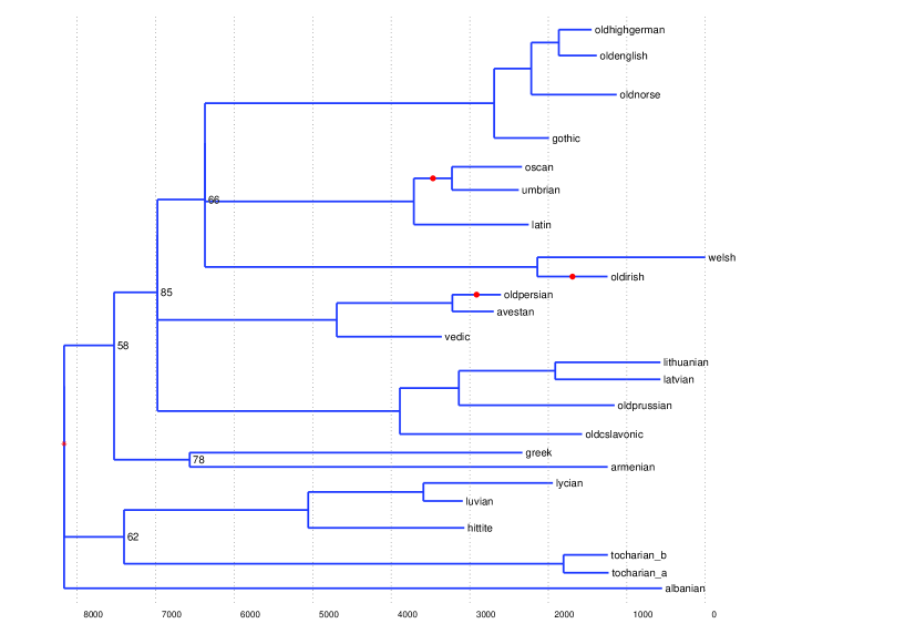
Figure 4: Consensus tree for the Ringe et al. (2002) dataset. Red dots show catastrophes supported with probability above one half.

We display in Figure 5 the calibration constraints on a tree sampled from the posterior. The constraints cannot be shown on a consensus tree, as slices across a consensus tree are not isochronous.

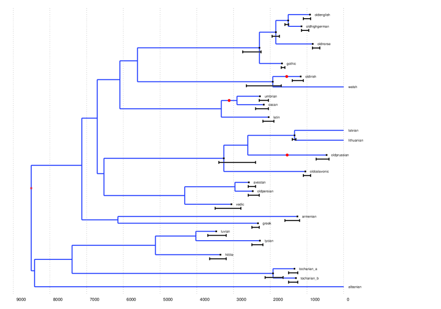
Figure 5: A typical sample from the posterior. All the constraints on the node ages are shown, except those for the Italic, Indo-Iranian and Iranian groups, for which we do not have an upper bound, and the root, which has an upper bound at $T=16000$ years BP.

The analysis reconstructs some well-known features of the Indo-European tree. The Germanic, Celtic and Italic families are grouped together, but no particular configuration of their relative positions is favored. The Indo-Persian group can fall outside the Balto-Slav group but the relative position of these two is uncertain. The deep topology of the tree is left quite uncertain by these data, especially the position of Albanian. We find evidence for catastrophic rate heterogeneity in three positions: on the edges leading to Old Irish, Old Persian, and in the Umbrian-Oscan clade.

Our estimate for the root age of the Indo-European family is 8430 $\pm$ 1320 years BP. The distribution of this key statistic is close to normal.

8 Conclusions

Our results give a root age for the most recent common ancestor of the Indo-European family of language vocabularies in agreement with earlier phylogenetic studies. Our results are in agreement with models which put this date around 8500 BP, and in conflict with models which require it to be less than 6500 years BP. Our studies of synthetic out-of-model data, and reconstruction tests for known historical data support our view that this main result is robust to model error. It would not be robust to a step change in the rate of lexical diversification acting in a coordinated fashion across the Indo-European languages extant some 3000 to 5000 years ago.

The methods outlined here for handling missing data and rate heterogeneity in the diversification of languages, as seen through lexical data, will find applications to generic trait data.

Appendix A Recursions for other registration processes

This section complements Section 3: we give iterations for $u_{i}^{(0)}$, $u_{i}^{(1)}$, $u_{i}^{(s_{i}-1)}$, $u_{i}^{(s_{i})}$, $v_{i}^{(s_{i}-1)}$ and $v_{i}^{(s_{i})}$. These are the quantities needed (as in Equation 3) to evaluate the sum in Equation 2, for registration rules which use Condition (1) in combination with other conditions from Section 2.3. Consider a pair of edges $\langle c_{1},i\rangle$, $\langle c_{2},i\rangle$ in $E$. In the notation of the text,

$$u_{i}^{(0)} = \left((1-\delta_{i,c_{1}})+\delta_{i,c_{1}}u_{c_{1}}^{(0)}\right)\left((1-\delta_{i,c_{2}})+\delta_{i,c_{2}}u_{c_{2}}^{(0)}\right)$$

$$u_{i}^{(1)} = \delta_{i,c_{1}}(1-\delta_{i,c_{2}})u_{c_{1}}^{(1)}+\delta_{i,c_{2}}(1-\delta_{i,c_{1}})u_{c_{2}}^{(1)}+\delta_{i,c_{1}}\delta_{i,c_{2}}(u_{c_{1}}^{(1)}u_{c_{2}}^{(0)}+u_{c_{1}}^{(0)}u_{c_{2}}^{(1)})$$

$$u_{i}^{(s_{i})} = \delta_{i,c_{1}}u_{c_{1}}^{(s_{c_{1}})}\delta_{i,c_{2}}u_{c_{2}}^{(s_{c_{2}})}$$

$$u_{i}^{(s_{i}-1)} = \left(\delta_{i,c_{1}}u_{c_{1}}^{(s_{c_{1}}-1)}+\mathbb{I}_{\{s_{c_{1}}=1\}}(1-\delta_{i,c_{1}})\right)\delta_{i,c_{2}}u_{c_{2}}^{(s_{c_{2}})}$$

$$\quad+\delta_{i,c_{1}}u_{c_{1}}^{(s_{c_{1}})}\left(\delta_{i,c_{2}}u_{c_{2}}^{s_{c_{2}}-1}+\mathbb{I}_{\{s_{c_{2}}=1\}}(1-\delta_{i,c_{2}})\right)\qquad$$

$$v_{i}^{(0)} = \left(\delta_{i,c_{1}}v_{c_{1}}^{(0)}+(1-\delta_{i,c_{1}})\prod_{j\in V_{L}^{c_{1}}}\xi_{j}\right)\left(\delta_{i,c_{2}}v_{c_{2}}^{(0)}+(1-\delta_{i,c_{2}})\prod_{j\in V_{L}^{c_{2}}}\xi_{j}\right)$$

$$v_{i}^{(s_{i})} = \left(\delta_{i,c_{1}}v_{c_{1}}^{(s_{c_{1}})}+(1-\delta_{i,c_{1}})\prod_{j\in V_{L}^{c_{1}}}(1-\xi_{j})\right)\left(\delta_{i,c_{2}}v_{c_{2}}^{(s_{c_{2}})}+(1-\delta_{i,c_{2}})\prod_{j\in V_{L}^{c_{2}}}(1-\xi_{j})\right)$$

$$v_{i}^{(s_{i}-1)} = \left(\delta_{i,c_{1}}v_{c_{1}}^{(s_{c_{1}}-1)}+(1-\delta_{i,c_{1}})s_{c_{1}}(1-\xi)^{s_{c_{1}}-1}\xi\right)\left(\delta_{i,c_{2}}v_{c_{2}}^{(s_{c_{2}})}+(1-\delta_{i,c_{2}})(1-\xi)^{s_{c_{2}}}\right)$$

$$+\ \left(\delta_{i,c_{1}}v_{c_{1}}^{(s_{c_{1}})}+(1-\delta_{i,c_{1}})(1-\xi)^{s_{c_{1}}}\right)\left(\delta_{i,c_{2}}v_{c_{2}}^{(s_{c_{2}}-1)}+(1-\delta_{i,c_{2}})s_{c_{2}}(1-\xi)^{s_{c_{2}}-1}\xi\right)$$

The recursion is evaluated from the leaves $i\in V_{L}$, at which

$$u_{i}^{(0)} = u_{i}^{(s_{i}-1)}=1-\xi_{i}$$

$$u_{i}^{(1)} = u_{i}^{(s_{i})}=\xi_{i}$$

$$v_{i}^{(0)} = v_{i}^{(s_{i}-1)}=0$$

$$v_{i}^{(s_{i})} = 1$$

References

- Alekseyenko et al. (2008) Alekseyenko, A., C. Lee, and M. Suchard (2008). Wagner and Dollo: A Stochastic Duet by Composing Two Parsimonious Solos. Systematic Biology 57(5), 772–784.
- Dyen et al. (1997) Dyen, I., J. Kruskal, and B. Black (1997). FILE IE-DATA1. Raw data available from http://www.ntu.edu.au/education/langs/ielex/IE-DATA1. Binary data available from http://www.psych.auckland.ac.nz/psych/research/RusselsData.htm.
- Felsenstein (1981) Felsenstein, J. (1981). Inferring phylogenies. Sinauer Associates Sunderland, Mass., USA.
- Garrett (2006) Garrett, A. (2006). Convergence in the formation of Indo-European subgroups: Phylogeny and chronology. Phylogenetic methods and the prehistory of languages, 139.
- Geyer (1992) Geyer, C. (1992). Practical Markov Chain Monte Carlo. Statistical Science 7(4), 473–483.
- Gray and Atkinson (2003) Gray, R. and Q. Atkinson (2003). Language-tree divergence times support the Anatolian theory of Indo-European origin. Nature 426(6965), 435–439.
- Lewis (2001) Lewis, P. (2001). A Likelihood Approach to Estimating Phylogeny from Discrete Morphological Character Data. Systematic Biology 50(6), 913–925.
- Mallory (1989) Mallory, J. (1989). In search of the Indo-Europeans: language, archaeology and myth. Thames and Hudson.
- McMahon and McMahon (2005) McMahon, A. and R. McMahon (2005). Language Classification by Numbers. Oxford University Press.
- Nicholls and Gray (2008) Nicholls, G. K. and R. D. Gray (2008). Dated ancestral trees from binary trait data and its application to the diversification of languages. Journal of the Royal Statistical Society, series B 70(3), 545–566.
- Raftery (1996) Raftery, A. (1996). Hypothesis testing and model selection. In W. Gilks, S. Richardson, and D. Spiegelhalter (Eds.), Markov Chain Monte Carlo in Practice. Chapman & Hall / CRC.
- Renfrew (1987) Renfrew, C. (1987). Archaeology and Language. The Puzzle of Indo-European Origins. Current Anthropology 29, 437–441.
- Ringe et al. (2002) Ringe, D., T. Warnow, and A. Taylor (2002). Indo-European and Computational Cladistics. Transactions of the Philological Society 100(1), 59–129.
- Ronquist et al. (2005) Ronquist, F., J. Huelsenbeck, and P. van der Mark (2005). MrBayes 3.1 Manual. School of Computational Science, Florida State University.
- Warnow et al. (2004) Warnow, T., S. Evans, D. Ringe, and L. Nakhleh (2004). A Stochastic model of language evolution that incorporates homoplasy and borrowing. Phylogenetic Methods and the Prehistory of Languages.