Rate description of Fokker-Planck processes with time-periodic parameters

Abstract

The large time dynamics of a periodically driven Fokker-Planck process possessing several metastable states is investigated. At weak noise transitions between the metastable states are rare. Their dynamics then represent a discrete Markovian process characterized by time dependent rates. Apart from the occupation probabilities, so-called specific probability densities and localizing functions can be associated to each metastable state. Together, these three sets of functions uniquely characterize the large time dynamics of the conditional probability density of the original process. Exact equations of motion are formulated for these three sets of functions and strategies are discussed how to solve them. These methods are illustrated and their usefulness is demonstrated by means of the example of a bistable Brownian oscillator within a large range of driving frequencies from the slow semiadiabatic to the fast driving regime.

1 Introduction

Chemical reactions have provided ubiquitous and versatile examples of activated transitions between two metastable states, formed by the reactants and products. In a chemical reaction the energy necessary for the activation most often stems from the (classical or even quantum mechanical) thermal energy that may accumulate in a single reaction coordinate and finally enable a transition from reactants to products [1, 2, 3, 4]. In contrast to these thermally assisted escape processes other additional sources of energy may externally be provided for example by driving a system with metastable states by periodic forces. Such periodically driven stochastic systems present a particular class of nonequilibrium processes that exhibit a broad variety of fascinating effects [5, 6, 7] such as stochastic resonance [8], directed transport of Brownian particles in ratchet type periodic potentials [9, 10, 11] or other anomalous transport properties as for example negative mobility [12]. Apart from an external periodic driving, these systems typically are subject to nonlinear dynamical laws and additionally experience fluctuating forces describing the random impact of the environment of the considered system [13]. Without the fluctuating forces the presence of nonlinearities often renders these systems multistable, i.e. such systems may approach different attractors [14], depending on their initial states. In combination with weak fluctuating forces these attractors become metastable states, which means that the system will be found most of the time in or close to one of these states while transitions between these states present rare events.

Each of the principal constituents of the dynamics of a periodically driven nonlinear stochastic system is characterized by typical time scales such as the correlation time of the fast random forces (ff), $\tau_{\text{ff}}$, relaxation times $\tau$ of the deterministic part of the dynamics, the period $T$ of the driving force and the times $\tau_{\text{ms}}$ of typical sojourn within the different metastable states (ms). In this work we will assume that the correlation times of the fluctuating forces are much shorter than all other time scales such that a Markovian description of the dynamics is appropriate. Hence, we model the fluctuating forces by white noise ($\tau_{\text{ff}}=0$) which moreover will be assumed to be Gaussian and weak. As a consequence of these assumptions the characteristic sojourn times of the metastable states are finite but much larger than any of the deterministic characteristic times ($\tau_{\text{ms}}\gg\tau$) [3]. This time scale separation implies that the transitions between the metastable states constitute a discrete Markovian process which will be investigated in more detail in the present work. We will demonstrate that this discrete process forms the backbone of the original continuous process on time scales that are much larger than the deterministic relaxation times $\tau$ .

Finally, the magnitude of the driving period $T$ in relation to the deterministic time scales $\tau$ has a decisive influence on the system’s dynamics. In the so-called semiadiabatic limit [15] the driving period is large compared to typical deterministic relaxation times independently of how large the driving period is compared with the typical sojourn times. Then the time-dependent transition rates are given by the frozen rates, i.e. their time dependence only results from the slow change of those system parameters that are varied by the driving process [16]. Within this framework stochastic resonance [17] and the dynamics of neuron models [18] have successfully been described.

Outside the regime of the so called semiadiabatic limit the escape rates no longer instantly follow but rather lack behind the periodic driving [19]. In the present paper we investigate this regime of intermediate to fast driving in more detail and present effective methods to characterize the large time behavior of periodically driven Fokker-Planck processes with metastable states.

Previous works on periodically driven processes with metastable states most often have been focussed on particular aspects such as on the dependence of the average life time of a metastable state [20, 21], of the exponentially leading part of escape rates within linear response theory [22], or on rates in the weak noise limit [23, 24].

We close this Introduction with a short outline of the paper. In Section 2 we introduce some important concepts of the deterministic dynamics of a periodically driven system with coexisting attractors. In Section 3 two alternative formulations of the conditional probability density function are presented for events that are separated by a time that is much larger than the characteristic deterministic time $\tau$. The first form originates from the Floquet representation of the conditional probability density of a periodically driven Markov process [5, 6] while the second expression explicitly refers to the dynamics of the metastable states. This second expression in particular contains quantities that characterize specific probability densities for each metastable state as well as localizing functions that allocate probabilities to the metastable states given the state of the full continuous system. In Section 4 we find equations of motion both for these metastable state specific probability densities and the localizing functions by comparing the two formulations of the conditional probability density at large times. In Section 5 the theory is exemplified and numerically tested for a bistable Brownian oscillator. Section 6 closes with a summary.

2 Characterization of the deterministic dynamics

In the deterministic limit the considered system is described by the motion of a state ${\mathbf{x}}$ in a $d$ dimensional state space $\Sigma$ governed by a set of $d$ coupled differential equations

$$\dot{{\mathbf{x}}}={\mathbf{f}}({\mathbf{x}},t)\>,$$ (1)

where the vector field ${\mathbf{f}}({\mathbf{x}},t)$ periodically depends on time with period $T$, i.e. ${\mathbf{f}}({\mathbf{x}},t+T)={\mathbf{f}}({\mathbf{x}},t)$. We denote the trajectory emanating at the time $s$ from the point ${\mathbf{y}}$ by ${\mathbf{X}}(t|{\mathbf{y}},s)$ and assume that in the asymptotic limit of large times the motion is bounded and characterized by a set of $n\geq 2$ different attractors $\mathcal{A}_{\alpha}(t)\subset\Sigma$, $\alpha=1\ldots n$, such that each trajectory approaches either of the attractors depending on its initial state and starting time, i.e. ${\mathbf{X}}(t|{\mathbf{y}},s)\to{\mathbf{x}}\in\mathcal{A}_{\alpha}(t)$ for $t-s$ sufficiently large. This relaxation process happens on a characteristic deterministic time scale of the considered system. The attractors periodically depend on time, i.e.

$$\mathcal{A}_{\alpha}(t+T)=\mathcal{A}_{\alpha}(t)\>.$$ (2)

To each attractor a domain of attraction $\mathcal{D}_{\alpha}(s)$ exists that consists of all states ${\mathbf{y}}$ at time $s$ from which the $\alpha^{\text{th}}$ attractor is reached. It is formally defined as $\mathcal{D}_{\alpha}(s)=\left\{{\mathbf{y}}|{\mathbf{X}}(t|{\mathbf{y}},s)\in\mathcal{A}_{\alpha}(t)\;\text{for}\;t-s\to\infty\right\}$. At each fixed time the domains of attraction form a partition of the state space into disjoint subsets, which in general periodically depend on time

$$\mathcal{D}_{\alpha}(t+T)=\mathcal{D}_{\alpha}(t)\>.$$ (3)

3 Conditional probability density of time-periodic Fokker-Planck processes with metastable states

3.1 Floquet representation

In many cases the description of a system in terms of deterministic equations of motion is sufficient in order to determine the typical behavior of the system with sufficient accuracy. However, the presence of weak random perturbations, which often can be modeled by Gaussian white noise, causes different effects depending on the considered time scales: On characteristic time scales of the deterministic motion only insignificant deviations from the deterministic motion typically occur; those trajectories that start close to the boundaries of the domains of attraction though are exceptional because they may be influenced even by small noise, cross the border of the deterministic domain of attraction and, in this way, come close to a “wrong” attractor with finite probability; all other trajectories are markedly influenced on much longer time scales only on which transitions between the deterministic, locally stable states become likely. Hence, these states lose their stability. Nevertheless, for sufficiently weak noise the system is found most of the time close to one of the formerly stable states. Transitions between these states do occur with certainty even though this happens rarely. Therefore such states can be considered as metastable.

Under the influence of Gaussian white noise the deterministic dynamical system (1) becomes a Markov process that is characterized by a Fokker-Planck operator of the following form [25, 26]

$$L(t)=-\sum_{i}^{d}\frac{\partial}{\partial x_{i}}K_{i}({\mathbf{x}},t)+\sum_{i,j}^{d}\frac{\partial^{2}}{\partial x_{i}\partial x_{j}}D_{i,j}({\mathbf{x}},t)\>.$$ (4)

We here will restrict ourselves to periodically driven processes where the drift $K_{i}({\mathbf{x}},t)$ and possibly also the diffusion $D_{i,j}({\mathbf{x}},t)$ periodically depend on time with a common period $T$. Hence, $L(t+T)=L(t)$. The time evolution of the system’s probability density function (pdf) $\rho({\mathbf{x}},t)$ is governed by the Fokker-Planck equation

$$\frac{\partial}{\partial t}\rho({\mathbf{x}},t)=L(t)\rho({\mathbf{x}},t)\>.$$ (5)

In the deterministic limit the diffusion matrix vanishes and the drift $K_{i}({\mathbf{x}},t)$ approaches the deterministic drift $f_{i}({\mathbf{x}},t)$ having the properties discussed in Section 1.

A particular solution of the Fokker-Planck equation is the conditional pdf $\rho({\mathbf{x}},t|{\mathbf{y}},s)$ to find the process at the state ${\mathbf{x}}$ at time $t$ under the condition that it was at the state ${\mathbf{y}}$ at time $s$. It can formally be expressed in terms of the Floquet representation in the following way [5, 6, 7, 8, 15]

$$\rho({\mathbf{x}},t|{\mathbf{y}},s)=\sum_{i}e^{\mu_{i}(t-s)}\psi_{i}({\mathbf{x}},t)\varphi_{i}({\mathbf{y}},s)\>,$$ (6)

where $\psi_{i}({\mathbf{x}},t)$ and $\varphi_{i}({\mathbf{y}},s)$ are Floquet eigenfunctions and $\mu_{i}$ are the corresponding Floquet exponents. They satisfy pairs of mutually adjoint Floquet equations reading

$$\begin{split}\frac{\partial}{\partial t}\psi_{i}({\mathbf{x}},t)&=L(t)\psi_{i}({\mathbf{x}},t)-\mu_{i}\psi_{i}({\mathbf{x}},t)\>,\\ -\frac{\partial}{\partial t}\varphi_{i}({\mathbf{x}},t)&=L^{+}(t)\varphi_{i}({\mathbf{x}},t)-\mu_{i}\varphi_{i}({\mathbf{x}},t)\>,\end{split}$$ (7)

with natural boundary conditions with respect to the state variable ${\mathbf{x}}$. Moreover, both types of eigenfunctions are periodic in time

$$\begin{split}\psi_{i}({\mathbf{x}},t+T)&=\psi_{i}({\mathbf{x}},t)\>,\\ \varphi_{i}({\mathbf{x}},t+T)&=\varphi_{i}({\mathbf{x}},t)\>.\end{split}$$ (8)

The Floquet functions $\psi_{i}({\mathbf{x}},t)$ and $\varphi_{j}({\mathbf{x}},t)$ are mutually orthogonal for eigenvalues $\mu_{i}\neq\mu_{j}$ and can be normalized such that

$$\int d{\mathbf{x}}\>\varphi_{j}({\mathbf{x}},t)\psi_{i}({\mathbf{x}},t)=\delta_{i,j}\>,$$ (9)

where $\delta_{i,j}$ denotes the Kronecker symbol. The Floquet exponents $\mu_{j}$ have real parts that are negative or at most zero.

The representation of the conditional probability in terms of the Floquet functions further requires that these functions form a complete set in the sense that

$$\sum_{i}\psi_{i}({\mathbf{x}},t)\varphi_{i}({\mathbf{y}},t)=\delta({\mathbf{x}}-{\mathbf{y}})\>,$$ (10)

where $\delta({\mathbf{x}})$ denotes the Dirac $\delta$ function. We note that equations (7), (9) and (10) do not uniquely determine the Floquet functions because gauge transformations of the form

$$\begin{split}\bar{\psi}_{j}({\mathbf{x}},t)&=g_{j}(t)\psi_{j}({\mathbf{x}},t)\>,\\ \bar{\varphi}_{j}({\mathbf{x}},t)&=g_{j}^{-1}(t)\varphi_{j}({\mathbf{x}},t)\>,\\ \bar{\mu}_{j}&=\mu_{j}+\frac{2\pi i}{T}n_{j},\quad n_{j}\in\mathbb{Z}\end{split}$$ (11)

with gauge factors

$$g_{j}(t)=c_{j}e^{2\pi in_{j}t/T}\>,\quad c_{j}\in\mathbb{C},\;c_{j}\neq 0$$ (12)

generate new Floquet eigenfunctions, cf. Ref. [27]. Here $\mathbb{Z}$ and $\mathbb{C}$ denote the sets of integer and complex numbers, respectively and $i$ the imaginary unit.

For the sake of definiteness we assume that the gauge chosen for the Floquet representation of the conditional pdf (6) is such that the Floquet exponents assume their smallest possible absolute values. The Floquet spectrum consisting of these Floquet exponents then contains the value $\mu_{0}=0$. We assume that this Floquet exponent is not degenerate [28] if the diffusion matrix is different from zero. The corresponding eigenfunction of $L^{+}(t)$ is constant with respect to ${\mathbf{x}}$ and $t$ and can be chosen as $\varphi_{0}({\mathbf{x}},t)=1$; the eigenfunction $\psi_{0}({\mathbf{x}},t)$ of $L(t)$ is a non-negative and normalized function giving the uniquely defined asymptotic pdf. Hence, it is the unique solution of the Fokker-Planck equation (5) that is approached at time $t$ from any initial state in the remote past at $s\to-\infty$. As a Floquet eigenfunction it is periodic in $t$. The normalization

$$\int_{\Sigma}d{\mathbf{x}}\>\psi_{0}({\mathbf{x}},t)=1$$ (13)

follows from eq. (9) together with the fact that $\varphi_{0}({\mathbf{x}},t)=1$.

For vanishing noise, the diffusion matrix $D_{i,j}({\mathbf{x}},t)$ vanishes and the backward operator becomes a first order partial differential operator $L^{+}_{0}(t)=\sum_{i}f_{i}({\mathbf{x}},t)\partial/\partial x_{i}$ with $f_{i}({\mathbf{x}},t)$ being the components of the deterministic vector field ${\mathbf{f}}({\mathbf{x}},t)$ governing the deterministic motion, eq. (1). For a dynamical system with $n$ coexisting attractors the characteristic functions of the domains of attraction represent $n$ independent periodic solutions of the backward equation $-\partial\varphi_{0}/\partial t=L_{0}^{+}(t)\varphi_{0}$. Each of the solutions is unity on one of the domains of attraction and zero outside. All other periodic solutions are linear combinations of these characteristic functions. That means that a deterministic system with $n$ locally stable states possesses an $n$-fold degenerate Floquet eigenvalue $\mu_{0}=0$. As discussed above, in the presence of noise, the formerly locally stable states become metastable. The $n$-fold degeneracy of $\mu_{0}=0$ is lifted, but at sufficiently weak noise there remains a group of $n$ Floquet exponents one of which is exactly zero and the others aquire a small negative real part. We call them the slow Floquet exponents. For sufficiently small noise this group of slow Floquet exponents stays well separated from all other Floquet exponents. For large time lags, the slow Floquet exponents and the corresponding Floquet eigenfunctions completely determine the conditional pdf which becomes

$$\begin{split}\rho({\mathbf{x}},t|{\mathbf{y}},s)&=\sum_{i=0}^{n-1}e^{\mu_{i}(t-s)}\psi_{i}({\mathbf{x}},t)\varphi_{i}({\mathbf{y}},s)\\ &\qquad\qquad\text{for}\;t-s\gg\tau\>,\end{split}$$ (14)

where the sum only runs over the group of $n$ slow Floquet exponents i.e. over those exponents with the smallest absolute values. All other Floquet exponents are determined by the deterministic time scales all of which are much shorter than those given by the slow Floquet exponents. Here $\tau$ denotes the slowest deterministic time scale.

3.2 Alternative representation of the conditional probability at large times

In the presence of metastable states the process of moving from a state ${\mathbf{y}}$ at time $s$ to a state ${\mathbf{x}}$ at a much later time $t$ may be subdivided into three consecutive steps that correspond to three contributions to the conditional probability $\rho({\mathbf{x}},t|{\mathbf{y}},s)$: Within the typical relaxation time $\tau$, compared to which the considered time span $t-s$ is supposed to be very large, the initial state ${\mathbf{y}}$ will be allocated to either of the metastable states $\beta$ with a probability $\chi_{\beta}({\mathbf{y}},s)$; within the remaining time $t-s-\tau\approx t-s$ the process may visit several other metastable states and will be found in the state $\alpha$ at the final time $t$ with a probability $p(\alpha,t|\beta,s)$. Given the final discrete state $\alpha$, the actual continuous states are distributed with a pdf $\rho({\mathbf{x}},t|\alpha)$. For sufficiently small noise the times within which the first and the last steps are performed are negligibly short compared to the total time $t-s$. Therefore, the initial allocation to a metastable state $\alpha$ and the final allocation to a continuous state ${\mathbf{x}}$ can be considered as instantaneous events. Moreover, all three steps are independent of each other and therefore the conditional probability $\rho({\mathbf{x}},t|{\mathbf{y}},s)$ results as

$$\rho({\mathbf{x}},t|{\mathbf{y}},s)=\sum_{\alpha,\beta}\rho({\mathbf{x}},t|\alpha)p(\alpha,t|\beta,s)\chi_{\beta}({\mathbf{y}},s)\>.$$ (15)

This particular form of the conditional pdf was derived in the semiadiabatic limit [16] which is definded by the regime for which the driving is slow compared to the characteristic local relaxation times but not necessarily slow compared to the typical transition times between metastable states [15]. We claim that this particular form of the conditional pdf remains to hold true also beyond the semiadiabatic limit, i.e. in situations when the driving period is comparable or even faster than the local relaxation times. The rare occurrence of the transitions between the metastable states is the only condition required for eq. (15) to hold. It implies the separation of the times needed to perform the first and the third step compared to the much larger time of the second step and justifies the independence of these three steps and their respective contributions to the conditional probability. Below, we will infer the main properties of these three sets of functions $\rho({\mathbf{x}},t|\alpha)$, $\chi_{\alpha}({\mathbf{x}},t)$ and $p(\alpha,t|\beta,s)$ from their according definitions.
(i) Each localizing function $\chi_{\alpha}({\mathbf{x}},t)$ assumes an almost constant value very close to unity within the domain of attraction $\mathcal{D}_{\alpha}(t)$ and vanishes outside. Close to the border of $\mathcal{D}_{\alpha}(t)$, the localizing function $\chi_{\alpha}({\mathbf{x}},t)$ smoothly interpolates between these two values. At each point ${\mathbf{x}}$ all $n$ functions $\chi_{\alpha}({\mathbf{x}},t)$ exactly add up to unity:

$$\sum_{\alpha}\chi_{\alpha}({\mathbf{x}},t)=1\>.$$ (16)

(ii) Each $\alpha$-specific pdf $\rho({\mathbf{x}},t|\alpha)$ is a strongly peaked function of ${\mathbf{x}}$ about the corresponding attractor $\mathcal{A}_{\alpha}(t)$ and rapidly decays away from the attractor. As pdf it is normalized to unity

$$\int_{\Sigma}d{\mathbf{x}}\>\rho({\mathbf{x}},t|\alpha)=1\>,$$ (17)

where the integration extends over the full state space $\Sigma$. Within the respective domains of attraction $\mathcal{D}_{\alpha}(t)$ the $\alpha$-specific pdf almost coincides with the asymptotic pdf $\psi_{0}({\mathbf{x}},t)$ up to a normalizing factor.

Property (i) of the localizing function allows one to determine the probability $p_{\alpha}(t)$ of finding the metastable state $\alpha$ realized at time $t$ for a given pdf $\rho({\mathbf{x}},t)$ in the following way

$$p_{\alpha}(t)=\int_{\Sigma}d{\mathbf{x}}\>\chi_{\alpha}({\mathbf{x}},t)\rho({\mathbf{x}},t)\>.$$ (18)

On the other hand, one can assign to a given set of probabilities $p_{\alpha}(t)$ a pdf $\rho_{p}({\mathbf{x}},t)$ by decorating the metastable states $\alpha$ with the $\alpha$-specific pdfs yielding

$$\rho_{p}({\mathbf{x}},t)=\sum_{\alpha}\rho({\mathbf{x}},t|\alpha)p_{\alpha}(t)\>.$$ (19)

In order that eqs. (18) and (19) are compatible with each other, i.e. that eq. (18) reproduces the prescribed probabilities $p_{\alpha}(t)$ for $\rho(t)=\rho_{p}(t)$, the localizing functions and the $\alpha$-specific pdfs must form a biorthonormal set of functions, i.e.

$$\int_{\Sigma}d{\mathbf{x}}\>\chi_{\alpha}({\mathbf{x}},t)\rho({\mathbf{x}},t|\beta)=\delta_{\alpha,\beta}\>.$$ (20)

For a Fokker-Planck process the time evolution of a pdf $\rho({\mathbf{x}},t)$ is determined by the conditional pdf according to

$$\rho({\mathbf{x}},t)=\int_{\Sigma}d{\mathbf{y}}\>\rho({\mathbf{x}},t|{\mathbf{y}},s)\rho({\mathbf{y}},s)\>.$$ (21)

For large time lags $t\!-\!s$ the conditional pdf can be written as in eq. (15). Using eqs. (15), (18) and (20) one obtains from eq. (21) for the propagation of the probabilities $p_{\alpha}(t)$

$$p_{\alpha}(t)=\sum_{\alpha,\beta}p(\alpha,t|\beta,s)p_{\beta}(s)\>.$$ (22)

This relation expresses the occupation probabilities of the metastable states at a time $t$ in terms of the corresponding probabilities at an earlier time $s$. Eq. (22) hence confirms the interpretation of $p(\alpha,t|\beta,s)$ as the conditional probability of the coarse grained process of the metastable, discrete states $\alpha=1\ldots n$.

In order to derive an equation of motion for the probabilities $p_{\alpha}(t)$ one differentiates both sides of eq. (18) with respect to time, uses the Fokker-Planck equation (5), and expresses the pdf by means of eq. (20) in terms of the probabilities $p_{\beta}(t)$. In this way one obtains

$$\begin{split}\dot{p}_{\alpha}(t)&=\int_{\Sigma}d{\mathbf{x}}\>\big{\{}\frac{\partial\chi_{\alpha}({\mathbf{x}},t)}{\partial t}\rho({\mathbf{x}},t)\\ &\quad+\chi_{\alpha}({\mathbf{x}},t)L(t)\rho({\mathbf{x}},t)\big{\}}\\ &=\sum_{\beta}k_{\alpha,\beta}(t)p_{\beta}(t)\>,\end{split}$$ (23)

where the time dependent rates $k_{\alpha,\beta}(t)$ are defined as

$$\begin{split}k_{\alpha,\beta}(t)&=\int_{\Sigma}d{\mathbf{x}}\>\frac{\partial\chi_{\alpha}({\mathbf{x}},t)}{\partial t}\rho({\mathbf{x}},t|\beta)\\ &\quad+\int_{\Sigma}d{\mathbf{x}}\>\chi_{\alpha}({\mathbf{x}},t)L(t)\rho({\mathbf{x}},t|\beta)\>.\end{split}$$ (24)

Eq. (16) implies that the sum over the first index of the rates vanishes, i.e. $\sum_{\alpha}k_{\alpha,\beta}(t)=0$. Therefore, eq. (23) can be brought into the familiar form of a master equation [29]

$$\dot{p}_{\alpha}(t)=\sum_{\beta\neq\alpha}k_{\alpha,\beta}(t)p_{\beta}(t)-\sum_{\beta\neq\alpha}k_{\beta,\alpha}(t)p_{\alpha}(t)\>.$$ (25)

We expect that for sufficiently low noise the quantities $k_{\alpha,\beta}(t)$ do not become negative for $\alpha\neq\beta$ and therefore represent proper rates. A formal proof of the positivity though is not available. Negative values of $k_{\alpha,\beta}(t)$ though would indicate a breakdown of the basic assumption that the long time behavior of the process is described by a rate process.

4 Localizing functions, $\alpha$-specific pdfs and transition rates

Comparing the two expressions (14) and (15) one finds that the $\alpha$-specific pdfs $\rho({\mathbf{x}},t|\alpha)$ can be expressed as linear combinations of the first $n$ Floquet eigenfunctions $\psi_{i}({\mathbf{x}},t)$ and the localizing functions $\chi_{\alpha}({\mathbf{x}},t)$ can be written in terms of $\varphi_{i}({\mathbf{x}},t)$. This leads to the linear relations

$$\rho({\mathbf{x}},t|\alpha) =\sum_{i=0}^{n-1}C_{i,\alpha}(t)\psi_{i}({\mathbf{x}},t)\>,$$ (26)

$$\chi_{\alpha}({\mathbf{x}},t) =\sum_{i=0}^{n-1}D_{\alpha,i}(t)\varphi_{i}({\mathbf{x}},t)\>,$$ (27)

where $C_{i,\alpha}(t)$ and $D_{\alpha,i}(t)$ are yet undetermined, time dependent coefficients. The orthogonality relations (9), (20) and the linear independence of the first $n$ Floquet eigenfunctions imply the following orthogonality relations of the coefficients $C_{i,\alpha}(t)$ and $D_{i,\alpha}(t)$:

$$\begin{split}\sum_{i}D_{\alpha,i}(t)C_{i,\beta}(t)&=\delta_{\alpha,\beta}\>,\\ \sum_{\alpha}C_{i,\alpha}(t)D_{\alpha,j}(t)&=\delta_{i,j}\>.\end{split}$$ (28)

For $i=0$ the normalization of the Floquet function $\psi_{0}({\mathbf{x}},t)$, see eq. (13), and of the $\alpha$-specific pdfs $\rho({\mathbf{x}},t|\alpha)$, see eq. (17), leads to

$$C_{0,\alpha}(t)=1.$$ (29)

Next we derive sets of coupled equations of motion for the localizing functions and the $\alpha$-specific pdfs.

4.1 Transition rates

Using the Floquet representation of the $\alpha$-specific pdfs and localizing functions, (26) and (27), in combination with the Floquet equations (7) we obtain for the rates from eq. (24)

$$\begin{split}k_{\alpha,\beta}(t)&=\sum_{i}\left(\dot{D}_{\alpha,i}(t)C_{i,\beta}(t)+D_{\alpha,i}\>\mu_{i}\>C_{i,\beta}(t)\right)\\ &=\sum_{i}\left(\dot{D}_{\alpha,i}(t)D^{-1}_{\beta,i}(t)+D_{\alpha,i}\>\mu_{i}\;D^{-1}_{\beta,i}(t)\right)\>,\end{split}$$ (30)

where we expressed the coefficient matrix $C_{i,\beta}(t)$ as the inverse of $D_{\beta,i}(t)$ by means of eq. (28). Assuming for the moment that the rates $k_{\alpha,\beta}(t)$ were known we can rewrite eq. (30) as of an equations of motion for the coefficients $D_{\alpha,i}(t)$ and $C_{i,\alpha}(t)$ reading

$$\dot{D}_{\alpha,i}(t) =\sum_{\beta}k_{\alpha,\beta}(t)D_{\beta,i}(t)-D_{\alpha,i}(t)\mu_{i}\>,$$ (31)

$$-\dot{C}_{i,\alpha}(t) =\sum_{\beta}C_{i,\beta}(t)k_{\beta,\alpha}(t)-\mu_{i}C_{i,\alpha}(t)\>.$$ (32)

It is interesting to note that these are just the Floquet equations of the master equation (25) and, moreover, that the slow Floquet exponents of the Fokker-Planck coincide with the Floquet exponents of the master equation. This is a consequence of the fact that the master equation specifies the transitions between the metastable states, and, therefore, represents the backbone of the long time evolution of the Fokker-Planck process.

With the help of eq. (31) and the Floquet equations (7) the following equations of motion for the $\alpha$-specific pdfs and the localizing functions are obtained

$$\frac{\partial}{\partial t}\rho({\mathbf{x}},t|\alpha) =L(t)\rho({\mathbf{x}},t|\alpha)-\sum_{\beta}k_{\beta,\alpha}(t)\rho({\mathbf{x}},t|\beta)\>,$$ (33)

$$-\frac{\partial}{\partial t}\chi_{\alpha}({\mathbf{x}},t) =L^{+}(t)\chi_{\alpha}({\mathbf{x}},t)-\sum_{\beta}k_{\alpha,\beta}(t)\chi_{\beta}({\mathbf{x}},t)\>.$$ (34)

These two sets of equations for the functions $\rho({\mathbf{x}},t|\alpha)$ and $\chi_{\alpha}({\mathbf{x}},t)$ are adjoint to each other such that the biorthonormality of the $\alpha$-specific and the localizing functions, see eq. (20), continues to hold for all times once it holds true at a particular instant of time. Eqs. (33) and (34) represent a central result of this work.

The set of coupled equations (33) can be interpreted as the motion of $n$ replicas of the original process. Each replica is labeled by one of the attractor indices $\alpha$. The corresponding processes are described by the Fokker-Planck equation (5) with additional source and sink terms, $\sum_{\beta\neq\alpha}k_{\beta,\alpha}(t)\rho({\mathbf{x}},t|\alpha)$ and $-\sum_{\beta\neq\alpha}k_{\beta,\alpha}(t)\rho({\mathbf{x}},t|\beta)$, respectively. This means that, say, the $\alpha$-process dies with probability $\sum_{\beta\neq\alpha}k_{\beta,\alpha}(t)\rho({\mathbf{x}},t|\beta)$ and instantly resurrects with probability $\sum_{\beta\neq\alpha}k_{\beta,\alpha}(t)\rho({\mathbf{x}},t|\alpha)$ such that the total probability $\int_{\Sigma}d{\mathbf{x}}\rho({\mathbf{x}},t|\alpha)$ of each replica is conserved for all times. A natural requirement on a process described by the set of eqs. (33) is the positivity of the probabilities $\rho({\mathbf{x}},t|\alpha)$. For an arbitrary choice of the rates $k_{\alpha,\beta}(t)$ this property generally will be violated in the course of time. Only for the correct choice of the transition rates the positivity is guaranteed to hold. In principle, it is this requirement which determines the rates $k_{\alpha,\beta}(t)$ on the basis of eq. (33).

In view of the fact that eqs. (33) and (34) are coupled sets of equations not only for the functions $\rho({\mathbf{x}},t|\alpha)$ and $\chi_{\alpha}({\mathbf{x}},t)$, respectively, but that in these equations also the time dependent rates $k_{\alpha,\beta}(t)$ are unknown, it would be very difficult to solve these equations exactly. Therefore appropriate approximation schemes have to be devised. This will be done in the remaining part of this Section.

4.2 Absorbing boundary approximation: $\alpha$-specific pdfs

Assuming the appropriateness of the rate description, i.e. in particular the positivity of $k_{\alpha,\beta}(t)$ for all $\alpha\neq\beta$, one can decompose the sum on the right hand side of eq. (33) into a sink term $-\sum_{\beta\neq\alpha}k_{\beta,\alpha}(t)\>\rho({\mathbf{x}},t|\beta)$ and a source term $\sum_{\alpha\neq\beta}k_{\beta,\alpha}(t)\>\rho({\mathbf{x}},t|\alpha)$. These sink and source terms result from the diagonal and non-diagonal parts of the rate matrix $(k_{\alpha,\beta}(t))$, respectively. The sink terms are linear combinations of the functions $\rho({\mathbf{x}},t|\beta)$, which are strongly concentrated about the positions of the corresponding attractors $\mathcal{A}_{\beta}(t)$ with $\beta\neq\alpha$.

We approximate these narrow, even though continuously distributed sink terms by replacing them with sharp, absorbing states lying on the boundaries $\partial\mathcal{B}_{\beta}(t)$ of domains $\mathcal{B}_{\beta}(t)$. Each domain $\mathcal{B}_{\beta}(t)$ contains the immediate neighborhood of the attractor $\mathcal{A}_{\beta}(t)$ in such a way that the boundary $\partial\mathcal{B}_{\beta}(t)$ separates the corresponding attractor from the remaining state space. Within this absorbing boundary approximation we obtain an uncoupled set of equations for the $\alpha$-specific pdfs reading

$$\begin{split}\frac{\partial}{\partial t}\bar{\rho}({\mathbf{x}},t|\alpha)&=L(t)\bar{\rho}({\mathbf{x}},t|\alpha)+k_{\alpha}(t)\bar{\rho}({\mathbf{x}},t|\alpha)\>,\\ &\qquad\text{for}\;{\mathbf{x}}\in\Sigma_{\alpha}(t)\>,\\ \bar{\rho}({\mathbf{x}},t|\alpha)&=0\>,\quad\text{for all}\;{\mathbf{x}}\in\partial\mathcal{B}_{\beta}(t)\;\text{with}\;\beta\neq\alpha\>,\end{split}$$ (35)

where

$$k_{\alpha}(t)\equiv-k_{\alpha,\alpha}(t)=\sum_{\beta\neq\alpha}k_{\beta,\alpha}(t)$$ (36)

denotes the total decay rate of the state $\alpha$ which is the sum over the individual rates from $\alpha$ to all other states $\beta$. The restricted state space $\Sigma_{\alpha}(t)$ is obtained from the full state space $\Sigma$ by excluding the immediate neighborhoods $\mathcal{B}_{\beta}(t)$ of all metastable states $\beta$ being different from $\alpha$. Hence, it is defined as

$$\Sigma_{\alpha}(t)\equiv\Sigma\smallsetminus\cup_{\beta\neq\alpha}\mathcal{B}_{\beta}(t)\>.$$ (37)

On this restricted state space the function $\bar{\rho}({\mathbf{x}},t|\alpha)$ is expected to represent a valid approximation of the $\alpha$-specific pdf $\rho({\mathbf{x}},t|\alpha)$.

We search for the periodic solution of eq. (35) which can be obtained in the following way. First one numerically solves the source free problem

$$\begin{split}\frac{\partial}{\partial t}\tilde{\rho}({\mathbf{x}},t|\alpha)&=L(t)\tilde{\rho}({\mathbf{x}},t|\alpha)\>,\\ \tilde{\rho}({\mathbf{x}},t|\alpha)&=0,\quad\text{for all}\;{\mathbf{x}}\in\partial\mathcal{B}_{\beta}(t)\;\text{with}\;\beta\neq\alpha\end{split}$$ (38)

with an initial condition that is positive in a small neighborhood of the attractor $\mathcal{A}_{\alpha}(t)$ and vanishes everywhere else. Because of the absorbing boundary conditions at $\partial\mathcal{B}_{\beta}(t)$, with $\beta\neq\alpha$, the auxiliary function $\tilde{\rho}({\mathbf{x}},t|\alpha)$ decays in time, i.e.

$$N_{\alpha}(t)=\int_{\Sigma_{a}(t)}d{\mathbf{x}}\>\tilde{\rho}({\mathbf{x}},t|\alpha)$$ (39)

is a decreasing function of time. Here the integral is extended over the restricted state space $\Sigma_{\alpha}(t)$ excluding the domains $\mathcal{B}_{\beta}(t)$, $\beta\neq\alpha$, as defined in eq. (37). The normalized function

$$\bar{\rho}({\mathbf{x}},t|\alpha)=\tilde{\rho}({\mathbf{x}},t|\alpha)/N_{\alpha}(t)$$ (40)

then satisfies the eq. (35) with the total outgoing rate given by

$$k_{\alpha}(t)=-\frac{\dot{N}_{\alpha}(t)}{N_{\alpha}(t)}\>.$$ (41)

The such constructed solution $\tilde{\rho}({\mathbf{x}},t)/N_{\alpha}(t)$ approaches a periodic function in time on the time scale of the deterministic dynamics, and presents an approximation to the $\alpha$-specific function $\rho({\mathbf{x}},t|\alpha)$. The other rates $k_{\beta,\alpha}(t)$ leaving the metastable state $\alpha$ follow from the flux associated with $\rho({\mathbf{x}},t|\alpha)$ through the boundaries $\partial\mathcal{B}_{\beta}(t)$

$$k_{\beta,\alpha}(t)=\int_{\partial\mathcal{B}_{\beta}(t)}d{\mathbf{S}}\cdot{\mathbf{j}}({\mathbf{x}},t|\alpha)\>,\quad\alpha\neq\beta\>,$$ (42)

where $d{\mathbf{S}}$ denotes the surface element on $\partial\mathcal{B}_{\beta}(t)$ pointing towards the metastable state $\mathcal{A}_{\beta}(t)$, and ${\mathbf{j}}({\mathbf{x}},t|\alpha)$ the probability current carried by the pdf $\bar{\rho}({\mathbf{x}},t|\alpha)$. Its components read

$$\begin{split}j_{i}({\mathbf{x}},t|\alpha)&=K_{i}({\mathbf{x}},t)\bar{\rho}({\mathbf{x}},t|\alpha)\\ &\quad-\sum_{l}\frac{\partial}{\partial x_{l}}D_{i,l}({\mathbf{x}},t)\bar{\rho}({\mathbf{x}},t|\alpha)\>.\end{split}$$ (43)

This is a generalization of the well known flux-over-population expression for the rate [3, 30, 31, 32]. The stationary flux carrying pdf of the classical flux-over-population expression is replaced by the flux carrying time-periodic pdf $\bar{\rho}({\mathbf{x}},t|\alpha)$ which is normalized to one, whence also the population is one. The decisive difference to the classical flux-over-population expression lies in the fact that in eq. (42) the flux is determined as the probability flowing per time directly into the final metastable state, which because of the surrounding absorbing boundary acts as an outlet, rather than through a “saddlepoint” or “bottleneck” on the common part of the separatrices $\partial\mathcal{D}_{\alpha}(t)$ and $\partial\mathcal{D}_{\beta}(t)$ of the initial and the final metastable state. In the time independent case both expressions coincide under the condition that a region containing the final metastable state and the bottleneck in question is free of sources [33]. In contrast, in the time-periodic case the probability current contains a periodic contribution which in general has a nonuniform phase, i.e. the phase depends on the location ${\mathbf{x}}$. Therefore, the instantaneous probability flux through the bottleneck in general differs from the flux into the outlet. A large portion of probability flowing through the bottleneck, say within the first half of the period may flow back during the second half of the period. Only the time averages over one period of the probabilities flowing through the bottleneck and into the outlet do coincide.

4.2.1 $\alpha$-Floquet functions and rates

The functions $\tilde{\rho}({\mathbf{x}},t|\alpha)$ which satisfy the Fokker-Planck equation (38) on the restricted state space $\Sigma_{\alpha}(t)$ defined in eq. (37) are closely related to the Floquet functions $\psi^{\alpha}({\mathbf{x}},t)$ of the Fokker-Planck operator restricted to $\Sigma_{\alpha}(t)$ with absorbing boundaries on the surfaces of the excluded regions $\mathcal{B}_{\beta}(t)$. These $\alpha$-Floquet functions, as we call them, are the solutions of the corresponding Floquet equations which read

$$\begin{split}\frac{\partial}{\partial t}\psi_{i}^{\alpha}({\mathbf{x}},t)&=L(t)\psi_{i}^{\alpha}({\mathbf{x}},t)-\mu_{i}^{\alpha}\psi_{i}^{\alpha}({\mathbf{x}},t)\\ &\qquad\text{for}\;{\mathbf{x}}\in\Sigma_{\alpha}(t)\>,\;n=1,2,\ldots\\ \psi_{i}^{\alpha}({\mathbf{x}},t)&=0\quad\text{for}\;{\mathbf{x}}\in\partial\mathcal{B}_{\beta}(t),\;\beta\neq\alpha\>.\end{split}$$ (44)

Because of the absorbing boundaries at all but one metastable states the Floquet spectrum consisting of the $\alpha$-Floquet eigenvalues $\mu_{i}^{\alpha}$ completely lies in the complex half plain with negative real part. We denote the $\alpha$-Floquet eigenvalue closest to zero by $\mu_{1}^{\alpha}$. The absolute value of the real parts of all other $\alpha$-Floquet eigenvalues are much larger, i.e. $|\mu_{1}^{\alpha}|\ll|\mu_{i}^{\alpha}|$ for all $i\neq 1$. In the deterministic limit $\mu_{1}^{\alpha}$ approaches zero, whereas all other $\alpha$-Floquet eigenvalues stay finite.

In terms of the $\alpha$-Floquet eigenfunctions the solution of eq. (38) becomes

$$\tilde{\rho}({\mathbf{x}},t|\alpha)=\sum_{i=1}c_{i}\>e^{\mu_{i}^{\alpha}t}\>\psi_{i}^{\alpha}({\mathbf{x}},t)\>,$$ (45)

where $c_{i}$ are constant coefficients whose values depend on the choice of the initial distribution. For times which are large on the deterministic time scale, all terms in the sum become negligibly small apart from the first term corresponding to $\mu_{1}^{\alpha}$. Hence, we obtain

$$\tilde{\rho}({\mathbf{x}},t|\alpha)\propto e^{\mu^{\alpha}_{1}t}\>\psi_{1}^{\alpha}({\mathbf{x}},t)\>,$$ (46)

and, by proper normalization

$$\bar{\rho}({\mathbf{x}},t|\alpha)=\frac{\psi_{1}^{\alpha}({\mathbf{x}},t)}{\int_{\Sigma_{\alpha}(t)}d{\mathbf{x}}\>\psi_{1}^{\alpha}({\mathbf{x}},t)}\>.$$ (47)

With eq. (41) the total rate $k_{\alpha}(t)$ follows as the negative logarithmic derivative of the normalization $\int_{\Sigma(t)}d{\mathbf{x}}\>\psi_{1}^{\alpha}({\mathbf{x}},t)$. It becomes

$$k_{\alpha}(t)=-\mu_{1}^{\alpha}+r_{\alpha}(t)\>,$$ (48)

where

$$r_{\alpha}(t)=-\frac{d}{dt}\ln\int_{\Sigma_{\alpha}(t)}d{\mathbf{x}}\>\psi_{1}^{\alpha}({\mathbf{x}},t)\>.$$ (49)

The average of $r_{\alpha}(t)$ over one period vanishes because $r_{\alpha}(t)$ is the derivative of a periodic function. Hence, with eq. (48) the $\alpha$-Floquet eigenvalue $\mu_{1}^{\alpha}$ is given by the negative averaged total rate.

If one performs the time derivative in eq. (49) one finds

$$\begin{split}r_{\alpha}(t)&=-\frac{\frac{d}{dt}\int_{\Sigma_{{\alpha}}(t)}d{\mathbf{x}}\>\psi_{1}^{\alpha}({\mathbf{x}},t)}{\int_{\Sigma_{{\alpha}}(t)}d{\mathbf{x}}\>\psi_{1}^{\alpha}({\mathbf{x}},t)}\\ &=-\frac{\int_{\Sigma_{{\alpha}}(t)}d{\mathbf{x}}\>\left[L(t)\psi_{1}^{\alpha}({\mathbf{x}},t)-\mu_{1}^{\alpha}\psi_{1}^{\alpha}({\mathbf{x}},t)\right]}{\int_{\Sigma_{\alpha}(t)}d{\mathbf{x}}\>\psi_{1}^{\alpha}({\mathbf{x}},t)}\\ &=\sum_{\beta\neq\alpha}\frac{\int_{\partial\mathcal{B}_{\beta}(t)}\sum_{i,j}dS_{i}\frac{\partial}{\partial x_{j}}D_{i,j}({\mathbf{x}},t)\psi_{1}^{\alpha}({\mathbf{x}},t)}{\int_{\Sigma_{\alpha}(t)}d{\mathbf{x}}\>\psi_{1}^{\alpha}({\mathbf{x}},y)}\\ &\quad+\mu_{1}^{\alpha}\\ &=\sum_{\beta\neq\alpha}k_{\beta,\alpha}(t)+\mu_{1}^{\alpha}\>.\end{split}$$ (50)

In the second equality the time derivative was performed. There, the time dependence of the domain $\Sigma_{\alpha}(t)$ does not contribute because the $\alpha$-Floquet function vanishes on the boundary $\partial\Sigma_{\alpha}(t)=\cup_{\beta\neq\alpha}\partial\mathcal{B}_{\beta}(t)$. The time derivative of $\psi_{1}^{\alpha}({\mathbf{x}},t)$ was expressed by eq. (44). In the next step the integral involving the Fokker-Planck operator was written by means of Gauss’ theorem in terms of surface integrals over the boundary of $\Sigma_{\alpha}(t)$. The terms in the sum on $\beta$ are the ratios of the probability fluxes through the boundaries $\partial\mathcal{B}_{\beta}(t)$ carried by the $\alpha$-Floquet function $\psi_{1}^{\alpha}({\mathbf{x}},t)$, see eq. (43), and the corresponding populations $\int_{\Sigma_{\alpha}(t)}d{\mathbf{x}}\>\psi_{1}^{\alpha}({\mathbf{x}},t)$. According to the eqs. (42) and (47) the terms in the sum on $\beta$ agree with the individual rates $k_{\beta,\alpha}(t)$.

4.3 Absorbing boundary approximations: Localizing functions

The same type of approximation as for the $\alpha$-specific pdfs may also be applied to the equations of motion for the localizing functions: By neglecting those terms on the right hand side of eq. (34) that are proportional to the rates $k_{\alpha,\beta}(t)$ with $\beta\neq\alpha$ and by introducing absorbing boundary condititions on the hypersurfaces $\partial\mathcal{B}_{\beta}(t))$, $\beta\neq\alpha$ we obtain a set of uncoupled equations for approximate $\alpha$-localizing functions $\bar{\chi}_{\alpha}({\mathbf{x}},t)$ reading

$$\begin{split}-\frac{\partial}{\partial t}\bar{\chi}_{\alpha}({\mathbf{x}},t)&=L^{+}(t)\bar{\chi}_{\alpha}({\mathbf{x}},t)+k_{\alpha}(t)\bar{\chi}_{\alpha}({\mathbf{x}},t)\>,\\ &\qquad\text{for}\;{\mathbf{x}}\in\Sigma_{\alpha}(t)\>,\\ \bar{\chi}_{\alpha}({\mathbf{x}},t)&=0\>,\quad\text{for all}\;{\mathbf{x}}\in\partial\mathcal{B}_{\beta}(t)\;\text{with}\;\beta\neq\alpha\>.\end{split}$$ (51)

This absorbing boundary approximation is again justified because the rates $k_{\alpha,\beta}(t)$ are much smaller than the inverse time scales of the deterministic dynamics which govern the motion within the domains of attraction. Moreover it is consistent with the above approximation for the $\alpha$-specific pdfs in the sense that the integrals of the products of the $\alpha$-specific and the respective localizing function are independent of time, i.e.

$$\frac{d}{dt}\int_{\Sigma_{\alpha}(t)}d{\mathbf{x}}\>\chi_{\alpha}({\mathbf{x}},t)\rho({\mathbf{x}},t|\alpha)=0\>,$$ (52)

as follows from eqs. (35) and (51). Note that the time dependence of the integration domain $\Sigma_{\alpha}(t)$ does not contribute because the integrand vanishes at the boundary. The biorthonormality of the localizing functions and specific pdfs cannot be strictly maintained within this approximation. The deviations though are expected to be exponentially small with respect to the noise strength because of the small overlap of these functions for different metastable states.

As in the case of the $\alpha$-specific functions the total decay rate $k_{\alpha}(t)$ need not be known in order to determine the $\alpha$-localizing functions. Rather one again may first determine an auxiliary function $\tilde{\chi}_{\alpha}({\mathbf{x}},t)$ as the solution of the source free equation

$$\begin{split}-\frac{\partial}{\partial t}\tilde{\chi}_{\alpha}({\mathbf{x}},t)&=L^{+}(t)\tilde{\chi}_{\alpha}({\mathbf{x}},t)\>,\\ \tilde{\chi}_{\alpha}({\mathbf{x}},t)&=0,\quad\text{for all}\;{\mathbf{x}}\in\partial\mathcal{B}_{\beta}(t)\;\text{with}\;\beta\neq\alpha\>.\end{split}$$ (53)

Because of the dissipative nature of the backward operator $L^{+}(t)$ it is convenient to integrate this equation backward in time. A forward integration easily may run into numerical problems because unavoidable errors would grow exponentially in time. As an appropriate final condition for $\tilde{\chi}_{\alpha}({\mathbf{x}},t_{0})$ one may choose a function which is constant on the domain of attraction $\mathcal{D}_{\alpha}(t_{0})$ and zero everywhere else. The solution of this final value problem will approach a periodic solution on the time scale of the deterministic dynamics. This asymptotic periodic solution must be normalized at each instant of time by the integral of its product with the corresponding $\alpha$-specific function to yield the required approximation of $\chi_{\alpha}({\mathbf{x}},t)$

$$\bar{\chi}_{\alpha}({\mathbf{x}},t)=\frac{\tilde{\chi}_{\alpha}({\mathbf{x}},t)}{Z_{\alpha}(t)}\>,$$ (54)

where

$$Z_{\alpha}(t)=\int_{\Sigma_{\alpha}(t)}d{\mathbf{x}}\>\tilde{\chi}_{\alpha}({\mathbf{x}},t)\bar{\rho}({\mathbf{x}},t|\alpha)\>.$$ (55)

Using the eqs. (35) and (53) one finds

$$k_{\alpha}(t)=\frac{\dot{Z}_{\alpha}(t)}{Z_{\alpha}(t)}\>.$$ (56)

This relation confirms that the function given by the eqs. (54) and (55) indeed is a solution of eq. (51).

5 Periodically driven Brownian bistable oscillator

In order to exemplify the theory developed above and to check its consistency we consider an overdamped bistable Brownian oscillator driven by an external force that varies periodically in time. We choose a bistable quartic potential $V(x,t)$ that depends periodically on time, see Fig 1.

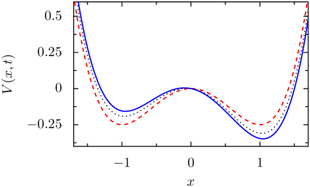
Figure 1: The bistable potential $V(x,t)$, eq. (57), is depicted as a function of the position $x$ for different times $t=0$ (red, dashed line), $t=0.2T$ (blue, solid line), and $t=0.4T$ (black, dotted line) where $T$ denotes the period of the driving and for the driving strength $A=0.1$.

In conveniently chosen dimensionless variables it reads

$$V(x,t)=-\frac{1}{2}x^{2}+\frac{1}{4}x^{4}-Ax\sin{\Omega t}\>,$$ (57)

where $t$ is time and $x$ the position of the Brownian particle. The strength of the periodic modulation is denoted by $A$ and its frequency by $\Omega$. Depending on the values of $A$ and $\Omega$ the deterministic overdamped dynamics in this time dependent potential is either monostable or bistable as displayed in Fig. 2. In the present context we are only interested in the bistable region in which the deterministic dynamics $\dot{x}=-V^{\prime}(x,t)$ possess two stable limit cycles $x_{-1}(t)$ and $x_{1}(t)$ and an unstable limit cycle $x_{0}(t)$ forming the separatrix between the two attractors, see Fig 3.

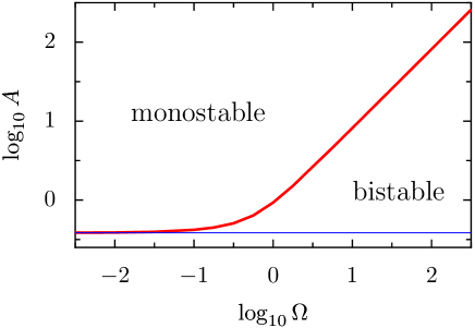
Figure 2: The line dividing the $\log_{10}\Omega$ – $\log_{10}A$ parameter plane into an upper monostable and a lower bistable region of the deterministic dynamics $\dot{x}=-V^{\prime}(x,t)$ is marked by the thick, red solid curve. The blue, thin straight line indicates the value of the forcing strength, $A^{\text{ad}}=2/(3\sqrt{3})$, below which the potential $V(x,t)$ has two minima for all times $t$.

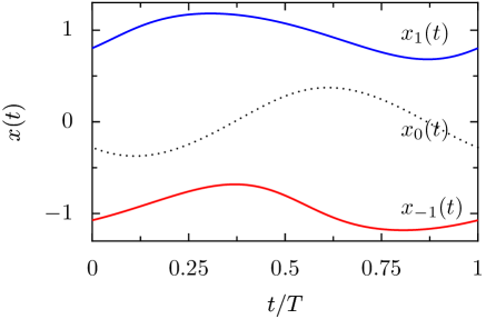
Figure 3: The attractors $x_{-1}(t)$, $x_{1}(t)$ and the separatrix $x_{0}(t)$ of the deterministic dynamics $\dot{x}=-V^{\prime}(x,t)$ for the driving strength $A=0.5$ and frequency $\Omega=1$.

The diffusion matrix $D$ is taken as constant. The Fokker-Planck operator then becomes

$$L(t)=\frac{\partial}{\partial x}V^{\prime}(x,t)+D\frac{\partial^{2}}{\partial x^{2}}\>,$$ (58)

where $V^{\prime}(x,t)$ denotes the derivative of the potential with respect to $x$. The corresponding Fokker-Planck and backward equations were numerically solved by a collocation method based on a representation of the solution in terms of Chebishev polynomials of degree 5 [34]. For all calculations a fixed number $N=1201$ of break-points in the interval $[-3,3]$ was used. At the ends of the interval reflecting boundary conditions were imposed. In the case of the forward equation an accuracy of $10^{-10}$ led to stable results whereas for the backward equations an accuracy of $10^{-12}$ turned out to be necessary in order to avoid numerical artefacts. Throughout this paper we used a fluctuation strength given by $D=1/40$. At vanishing driving strength $A=0$ the resulting bistable symmetric potential then possesses a barrier height per noise energy of $\Delta V/D=\left[V(0,0)-V(1,0)\right]/D=10$.

5.1 Flux-over-population rates

We first numerically determined the time dependent solution $\tilde{\rho}(x,t|-1)$ of the Fokker-Planck equation (38) on the restricted state space $\Sigma_{-1}(t)=[-3,x_{1}(t)]$ with a reflecting boundary at $x=-3$ and an absorbing boundary at the the position of the right attractor $x_{1}(t)$ and with an initial condition that is sharply located at the position of the other attractor $x_{-1}(0)$. After a number $n$ of periods $T=2\pi/\Omega$ of the driving frequency $\Omega$ had elapsed the remaining population $N_{-1}(t)$ was identified as

$$N_{-1}(t)=\int_{-3}^{x_{1}(t)}dx\>\tilde{\rho}(x,t|-1),$$ (59)

see also eq. (39), and the renormalized pdf

$$\bar{\rho}(x,t|-1)=\tilde{\rho}(x,t|-1)/N_{-1}(t)\>,$$ (60)

as well as the rate

$$k_{1,-1}(t)=-\frac{\dot{N}_{-1}(t)}{N_{-1}(t)}$$ (61)

were determined. The number $n$ of transient periods was chosen such that $k_{1,-1}(t)$ remained unchanged upon a further increase of $n$. For different values of $\Omega$ appropriate numbers $n$ are collected in Table 1.

Table 1: Number of transient periods

$\Omega$	$n$
1	100
0.5	50
0.1	10
0.01	5
0.001	3

In Fig. 4 the rates $k_{1,-1}(t)$ are displayed as functions of time for various driving frequencies. For small frequencies the time dependent rate approaches its adiabatic form [16] that is given by the inverse mean first time that a process needs to move from $x=x_{-1}(t)$ to $x=x_{1}(t)$ in the frozen potential. The rate then reads [3]

$$k^{\text{ad}}_{1,-1}(t)=D\left[\int_{x_{-1}(t)}^{x_{1}(t)}dx\>e^{V(x,t)/D}\int_{-3}^{x_{0}(t)}dy\>e^{-V(y,t)/D}\right]^{-1}.$$ (62)

For larger frequencies the maximal value of the rate shrinks and also becomes delayed with respect to the driving force. In the limit of high frequencies it approches the time independent rate $k^{\text{av}}$ of a Brownian particle moving in the potential $\overline{V(x,t)}=T^{-1}\int_{0}^{T}dt\>V(x,t)$ averaged over one period of the driving force. For the potential given by eq. (57) the average is symmetric and given by $\overline{V(x,t)}=V(x,0)$. Hence the rate in the limit of high driving frequencies coincides with the value of the adiabatic rate at $t=0$:

$$k^{\text{av}}=k^{\text{ad}}_{1,-1}(0)\>.$$ (63)

Due to the symmetry of the averaged potential, the rate $k^{\text{av}}$ also describes the opposite transition from the state $x_{1}(t)$ to $x_{-1}(t)$, whence we skipped the index.

At a fixed frequency the rate $k_{1,-1}(t)$ decreases with decreasing amplitude $A$ approaching the time independent value $k^{\text{av}}$, see Fig. 5

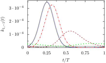
Figure 4: The rate $k_{1,-1}(t)$ following from eq. (61) displays a maximum as a function of $t/T$ that becomes lower and shifts towards later times within one period if the frequency $\Omega$ increases. For the frequency $\Omega=10^{-3}$ the rate is indistinguishable from the adiabatic rate (62) (black, solid line). The other curves display the rates for $\Omega=10^{-2}$ (blue, dotted line), $0.1$ (red, dash-dotted line), $0.5$ (brown, dashed line) and $1$ (green, thick dots); in the asymptotic limit $\Omega\to\infty$ the constant rate $k^{\text{av}}$ (thin solid line) given by eq. (63) is approached. In all cases the driving strength is $A=0.1$ and the noise strength $D=0.025$.

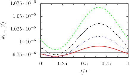
Figure 5: The times at which the rate $k_{1,-1}(t)$ assumes its extrema do hardly depend on the amplitude $A$. The rate is displayed for various values of $A=0.1$ (solid, red), $0.2$ (dotted, blue), $0.3$ (dashdotted, black), and $0.4$ (dashed, green); in all cases the frequency is $\Omega=10$, and the noise $D=0.025$. Note that for the large amplitude $A=0.4>A^{\text{ad}}$ the deterministic attractors $x_{\pm 1}(t)$ are dynamically stabilized, see also Fig. 2.

The specific pdf $\bar{\rho}(x,t|-1)$ given by eq. (60) represents a periodic current carrying pdf with an absorbing state at the attractor $x_{1}(t)$. It possesses a single maximum the location of which closely follows the deterministic motion of the attractor $x_{-1}(t)$, see Fig. 6. The pdf is asymmetric about its maximum with a breathing width that is wider if the maximum is closer to the position of the separatrix $x_{0}(t)$.

The approximate localizing function $\bar{\chi}_{-1}(x,t)$ of the left metastable state $x_{-1}(t)$ on the restricted state space $\Sigma_{-1}(t)$ was obtained from the solution $\tilde{\chi}_{-1}(x,t)$ of the backward equation (53) with absorbing boundary condition at the right metastable state $x_{1}(t)$. In order to guarantee for sufficient numerical stability, the integration of the backward equation has to be performed backward in time from some $t_{0}$ to times $t<t_{0}$. The final function $\tilde{\chi}_{-1}(x,t_{0})$ was chosen such that it assumes the constant value $1$ for all $x\in[-3,x_{-1}(t_{0})]$ then decreases monotonically and reaches zero at the right metastable state.

After the same number $n$ of transient periods as for the corresponding characteristic pdf, see Table 1, the normalization integral (55)

$$Z_{-1}(t)=\int_{-3}^{x_{1}(t)}dx\>\tilde{\chi}_{-1}(x,t)\bar{\rho}(x,t|-1)$$ (64)

was determined. The rates $k_{1,-1}(t)$ that follow from the logarithmic derivative of $Z_{-1}(t)$, cf. eq. (56), were compared with the rates obtained from eq. (61). They are identical within numerical accuracy.

Finally, the localizing function $\bar{\chi}_{-1}(x,t)$ was determined by normalizing $\tilde{\chi}_{-1}(x,t)$ with $Z_{-1}(t)$. For an example see Fig. 7. We note that the position where the localizing function assumes the value $1/2$ coincides with the location of the separatrix at the respective time.

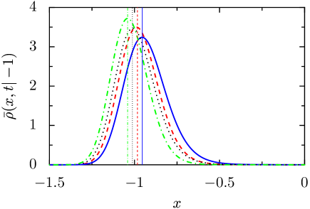
Figure 6: The specific pdf $\bar{\rho}(x,t|-1)$ is depicted as a function of the position $x$ for various times $t=0.12\>T$ (red, dashed), $0.37\>T$ (blue, solid), $0.62\>T$ (black, dotted), and $0.87\>T$ (green, dashed-dotted) for the driving frequency $\Omega=1$, driving amplitude $A=0.1$ and noise strength $D=0.025$. Outside the displayed interval the specific pdf continues to decay. It vanishes at the position of the attractor $x_{1}(t)$. The vertical lines indicate the positions of the attractor $x_{-1}(t)$ at the respective times. These positions almost coincide with the maxima of the specific pdfs at the respective times.

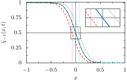
Figure 7: The localizing function $\bar{\chi}_{-1}(x,t)$ interpolates between the values $1$ at the attractor $x_{-1}(t)$ and $0$ at $x_{1}(t)$. It is displayed at various instants of time, $t=0.12\>T$ (red, dashed), $0.37\>T$ (blue, solid), $0.62\>T$ (black, dotted), and $0.87\>T$ (green, dash-dotted). The vertical lines denote the positions of the separatrix of the deterministic dynamics at the corresponding times, see Fig. 3. In the inset a magnification of the center part of the plot marked by a rectangle is depicted. It demonstrates that the localizing functions very precisely assume the value $1/2$ (horizontal line) at the positions of the separatrices indicated by the vertical lines.

5.2 Floquet approach

Here we construct the specific pdfs and the localizing functions in terms of Floquet eiegenfunctions on the basis of the eqs. (26) and (27). In the present case of two metastable states these equations simplify to read

$$\rho(x,t|\pm 1) =\psi_{0}(x,t)+C_{\pm 1}(t)\psi_{1}(x,t)\>,$$ (65)

$$\chi_{\pm 1}(x,t) =\frac{C_{\mp 1}(t)}{C_{\mp 1}(t)-C_{\pm 1}(t)}$$

$$\quad-\frac{1}{C_{\mp 1}(t)-C_{\pm 1}(t)}\varphi_{1}(x,t)\>.$$ (66)

Here we skipped the first index $i$ of $C_{i,\alpha}(t)$ since only the values for $i=1$ are nontrivial in the case of two metastable states. For $i=0$, $C_{0,\alpha}(t)=1$ always holds, see eq. (29).

To further evaluate these equations (i) the first two Floquet functions of the forward and the backward equation and (ii) the coefficients $C_{\pm 1}(t)$ were determined numerically. The Floquet function $\psi_{0}(x,t)$ belonging to the Floquet eigenvalue $\mu_{0}=0$ is the periodic solution of the Fokker-Planck equation (5), (58) with reflecting boundary conditions at $x=\pm 3$. As initial condition we chose

$$\psi_{0}(x,0)=\frac{\exp\left(-V(x,0)/D\right)}{\int_{-3}^{3}dx\exp\left(-V(x,0)/D\right)}\>.$$ (67)

The Fokker-Planck equation was numerically solved for $n$ periods of the driving force. We designated this number $n$ in such a way that after subsequent $n/10$ periods the $L_{1}$-norm of the difference of the two solutions was less than $10^{-5}$, i.e.

$$||\psi_{0}(x,1.1\>n\>T)-\psi_{0}(x,n\>T)||_{1}\leq 10^{-5}\>,$$ (68)

where the $L_{1}$-norm of a function $f(x)$ on the interval $[-3,3]$ is defined by the integral of the its absolute value as

$$||f(x)||_{1}=\int_{-3}^{3}dx|f(x)|\>.$$ (69)

The numbers $n$ found in this way are collected in Table 2 for different values of the driving frequency.

Table 2: Number of transient periods needed to reach convergence of the Floquet function $\psi_{0}(x,t)$ and Floquet exponent $\mu_{1}$

$\Omega$	$n$	$\mu_{1}$
1	10000	- 4.46 $10^{-5}$
0.5	2000	-  9.46 $10^{-5}$
0.1	1000	- 1.54 $10^{-4}$
0.01	1000	- 1.58 $10^{-4}$
0.001	100	- 1.58 $10^{-4}$

The Floquet function $\psi_{1}(x,t)$ and the corresponding Floquet exponent $\mu_{1}$ were obtained from the solution of the Fokker-Planck equation (5), (58) with reflecting boundary conditions at $x=\pm 3$ and the initial condition

$$\tilde{\psi}_{1}(x,0)=\delta\big{(}x-x_{-1}(0)\big{)}\>.$$ (70)

After a transient period of duration $n\>T$ with $n$ given by Table 1 the logarithm of the $L_{1}$-norm of the difference between $\tilde{\psi}_{1}(x,t)$ and $\psi_{0}(x,t)$ was plotted as a function of time for several periods. Its logarithm $\ln||\tilde{\psi}_{1}(x,t)-\psi_{0}(x,t)||_{1}$ is the superposition of a declining linear and a periodic function of time with period $T$ of the driving. The Floquet exponent $\mu_{1}$ can be read off from the inclination of the linear contribution. The results are presented in Table 2. We note here that the method of the $\alpha$-Floquet functions defined on a restricted phase space with an absorbing state at, say $x_{1}(t)$, see Section 4.2.1, gave Floquet exponents $\mu_{1}^{-1}$ which coincide with those based on the full state space up to 4 or 5 digits. The same agreement was obtained from the time average of the rates obtained by either of the methods described in the previous Section 5.1. Once the Floquet exponent $\mu_{1}$ is known, the still unnormalized Floquet eigenfunction is obtained as

$$\psi_{1}(x,t)=e^{-\mu_{1}t}\left(\tilde{\psi}_{1}(x,t)-\psi_{0}(x,t)\ \right)\>.$$ (71)

The first two Floquet eigenfunctions, which were normalized with respect to the $L_{1}$-norm, are displayed in Fig. (8).

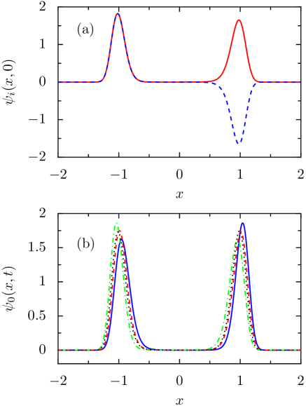
Figure 8: The first two Floquet eigenfunctions $\psi_{0}(x,0)$ (red, solid line) and $\psi_{1}(x,0)$ (blue, dashed line) of the Fokker-Planck operator (58) of a driven Brownian oscillator in a bistable potential (57) for the driving strengths $A=0.1$, driving frequency $\Omega=1$ and noise strength $D=2.5\times 10^{-2}$ at $t=0$ that are displayed in panel (a) are strongly localized in the vicinity of the two metastable states at $x_{\pm 1}(0)$. Both functions are normalized such that their $L_{1}$-norms are one, i.e. $||\psi_{i}(x,t)||_{1}=\int_{-3}^{3}dx|\psi_{i}(x,t)|=1$. The two functions almost agree with each other up to a change in sign close to the unstable point $x_{0}(0)$. In panel (b), the time dependence is indicated for the asymptotic pdf $\psi_{0}(x,t)$ for four different times $0.12T$ (red, dashed line), $0.37T$ (blue, solid line), $0.62T$ (black, dotted line) and $0.87T$ (green, dash-dotted line).

The Floquet eigenfunction of the backward operator belonging to the Floquet exponent $\mu_{0}=0$ is known to be constant, i.e. $\varphi_{0}(x,t)=1$. In order to determine the Floquet eigenfunction $\varphi_{1}(x,t)$ belonging to $\mu_{1}$ we solved the backward equation

$$-\frac{\partial}{\partial t}\tilde{\varphi}_{1}(x,t)=L^{+}(t)\tilde{\varphi}_{1}(x,t)$$ (72)

with the initial condition

$$\tilde{\varphi}_{1}(x,0)=\text{sign}(x)\cdot\left\{\begin{array}[]{ll}-1&|x|\geq 0.1\\ 100\cdot(|x|-0.1)^{2}-1&|x|\leq 0.1\>.\end{array}\right.$$ (73)

After a transient time of duration $nT$ with $n$ given in Table 1 all contributions from higher Floquet functions have become negligible and $\tilde{\varphi}_{1}(x,t)$ assumes the form

$$\tilde{\varphi}_{1}(x,t)=c_{0}+e^{\mu_{1}t}c_{1}\varphi_{1}(x,t)\>.$$ (74)

Knowing the Floquet exponent $\mu_{1}$ we determined the constant $c_{0}$ such that $[\tilde{\varphi}_{1}(x,t)-c_{0}]\exp(-\mu_{1}t)$ becomes a periodic function of time which is proportional to the sought-after function $\varphi_{1}(x,t)$. The normalization of $\varphi_{1}(x,t)$ is chosen such that

$$\int_{-3}^{3}dx\>\varphi_{1}(x,t)\psi_{1}(x,t)=1\>.$$ (75)

The spatial and temporal dependence of $\varphi_{1}(x,t)$ is depicted in Fig. 9 for the same parameter values as for the periodic pdf displayed in Fig. 8.

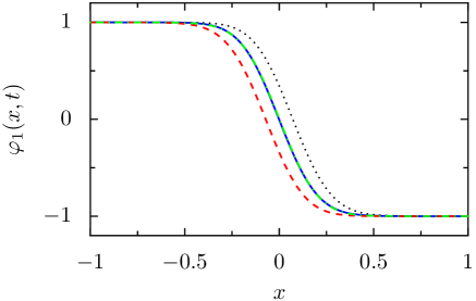
Figure 9: The Floquet eigenfunctions $\varphi_{1}(x,t)$ of the backward operator for the times $0.12T$ (red, dashed line), $0.37T$ (blue, solid line), $0.62T$ (black, dotted line) and $0.87T$ (green, dash-dotted line) are almost constant apart from a narrow region about the unstable fixed point $x_{0}(t)$. The parameters are with $A=0.1$, $\Omega=1$ and $D=2.5\times 10^{-2}$ the same as in Fig. 8.

Once the Floquet functions $\psi_{i}(x,t)$ for $i=0,1$ are known the coefficients $C_{\pm 1}(t)$ can be determined from the condition that the $\alpha$-specific pdf $\rho(x,t|\alpha)$ is negligibly small in the vicinity of the other metastable state $x_{\beta}(t)$ ($\alpha\neq\beta$). Hence the intergration on both sides of eq. (65) over a small neighborhood of $x_{\mp}(t)$ gives a negligibly small contribution and thus leads to the following expression for the coefficients $C_{\pm 1}(t)$

$$C_{\pm 1}(t)\approx-\frac{\int_{x_{\mp 1}(t)-\epsilon/2}^{x_{\mp 1}(t)+\epsilon/2}dx\>\psi_{0}(x,t)}{\int_{x_{\mp 1}(t)-\epsilon/2}^{x_{\mp 1}(t)+\epsilon/2}dx\>\psi_{1}(x,t)}\>.$$ (76)

As an example the coefficient $C_{-1}(t)$ is displayed in Fig. 10 for different values of the driving frequency. The interval length was chosen as $\epsilon=0.1$.

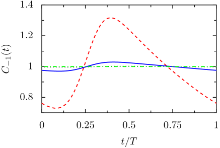
Figure 10: The variability of the coefficient $C_{-1}(t)$ within one period $T$ of the driving decreases with increasing frequency $\Omega=10^{-3}$ (red, dashed), $10^{-2}$ (blue, solid), $10^{-1}$ (black, dotted) and $1$ (green, dash-dotted). The other parameters are with $A=0.1$ and $D=2.5\times 10^{-2}$ the same as in Fig. 8.

Once the first two Floquet eigenfunctions and the coefficients $C_{\pm 1}(t)$ are known, the specific pdfs $\rho(x,t|\pm 1)$ and the localizing functions $\chi_{\pm 1}(x,t)$ can be calculated and compared with the results for $\bar{\rho}(x,t|\pm 1)$ and $\bar{\chi}_{\pm 1}(x,t)$, respectively, obtained by the flux-over-population method. We here restrict ourselves to a comparison for the specific pdf $\rho(x,t|-1)$ for fast driving with $\Omega=1$. Fig. 11 demonstrates the perfect agreement. Only in the immediate vicinity of the metastable state a difference becomes visible upon strong magnification.

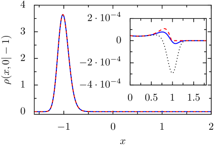
Figure 11: The specific pdf $\rho(x,0|-1)$ was determined by three different methods: As the flux carrying periodic pdf $\bar{\rho}(x,t|-1)$ in the presence of a sharp absorbing boundary at $x_{1}(t)$ (red, dashed line), and as a linear combination of the first two Floquet eigenfunctions, see eq. (65), with coefficients either determined by eq. (76) (blue, solid line), or from the solutuion of the Floquet problem of the master equation (black, dotted line), see the discussion below. Only in the magnification displayed in the inset a deviation of the results of these methods becomes visible in the vicinity of the metastable state $x_{1}(0)\approx 0.98$ where $\bar{\rho}(x_{0}(0),0|-1)=0$. We expect that these small deviations become even smaller at smaller noise strength.

Moreover, from the coefficients $C_{\pm 1}(t)$ and the Floquet exponent $\mu_{1}$ the rate $k_{-1,1}(t)$ and $k_{1,-1}(t)$ can be determined according to eq. (32) which simplifies for $k_{1,-1}(t)$ in the case of two metastable states to

$$k_{1,-1}(t)=\frac{\mu_{1}C_{-1}(t)-\dot{C}_{-1}(t)}{C_{1}(t)-C_{-1}(t)}\>.$$ (77)

A comparison of these rates with those obtained by the reactive flux method is presented in Fig. 12 for different values of the driving frequency. A qualitatively good agreement is obtained for all frequencies whereby deviations become more visible for higher frequencies.

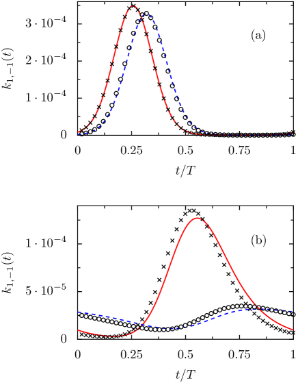
Figure 12: A comparison of the flux-over-population rates (fop rates) (lines) with the Floquet rate expressions (F rates) following from eq. (77) (symbols) is presented for frequencies $\Omega=0.01$ (fop rates: red, solid line; F rates: crosses) and $\Omega=0.1$ (fop rates: blue, dashed line; F rates: circles) in panel (a), and for $\Omega=0.5$ (fop rates: red, solid line; F rates: crosses) and $\Omega=1$ (fop rates: blue, dashed line; F rates: circles) in panel (b). The remaining parameters are with $A=0.1$, $D=2.5\times 10^{-2}$ the same as in Fig. 8.

5.3 Decoration

Finally, we numerically investigated the crucial assumption that after a sufficiently large transient period the pdf $\rho({\mathbf{x}},t)$ takes the form of eq. (19), i.e. it is determined by the solutions of the master equation (25), $p_{\alpha}(t)$, which are decorated by the $\alpha$-specific pdfs $\rho({\mathbf{x}},t|\alpha)$. As a quantitative measure of the distance between the numerically exact solution $\rho(x,t)$ of the Fokker-Planck equation (5), with the Fokker-Planck operator (58), starting at the metastable state $x_{-1}(0)$, i.e. with the initial condition (70), and an approximate form $\rho_{\text{a}}(x,t)$ of the pdf we employed the $L_{1}$-norm (69) of the difference of these functions. The assumed asymptotic form

$$\rho_{\text{a}}(x,t)=\rho(x,t|1)p_{1}(t)+\rho(x,t|-1)p_{-1}(t)$$ (78)

requires the knowledge of the probabilities $p_{\pm 1}(t)$ which was obtained as the solution of the master equation

$$\begin{split}\dot{p}_{1}(t)&=-k_{-1,1}(t)p_{1}(t)+k_{1,-1}(t)p_{-1}(t)\\ \dot{p}_{-1}(t)&=k_{-1,1}(t)p_{1}(t)-k_{1,-1}(t)p_{-1}(t)\\ p_{1}(0)&=0\>,\quad p_{-1}(0)=1\>,\end{split}$$ (79)

where the flux-over-population expressions were taken for the rates, see Section 5.1. For the specific pdfs we employed three different approximations: First we used the current carrying pdfs $\bar{\rho}(x,t|\pm 1)$ introduced in Section 5.1. These functions were extended onto the full state space $[-3,3]$ by assigning the value zero beyond their respective domains of definition, i.e. we defined

$$\begin{split}\rho_{I}(x,t|\!-\!1)&=\left\{\begin{array}[]{ll}\bar{\rho}(x,t|\!-\!1)&\text{for}\;-3\leq x\leq x_{1}(t)\\ 0&\text{for}\;x_{1}(t)\leq x\leq 3\end{array}\right.\\ \rho_{I}(x,t|1)&=\left\{\begin{array}[]{ll}0&\text{for}\;-3\leq x\leq x_{-1}(t)\\ \bar{\rho}(x,t|1)&\text{for}\;x_{-1}(t)\leq x\leq 3\>.\end{array}\right.\end{split}$$ (80)

As a second and third approximation, in the followowing referred to as approximation II and III, we used the specific pdfs (65) with the numerically determined Floquet functions, see Section 5.2, and determined the coefficients $C_{\pm 1}(t)$ in two different ways. The approximation II was obtained by using eq. (76) for the coefficients $C_{\pm 1}(t)$. The approximation III is based on the fact that these coefficients obey the Floquet equations (32) of the backward master equation. We numerically solved these equations under the assumption that the rates are given by the flux-over-population expressions. The resulting functions $c_{\pm 1}(t)$ then coincide with the sought-after coefficients $C_{\pm 1}(t)=qc_{\pm 1}(t)$ up to a common proportionality constant $q$. Finally this coefficient was determined such that the distance between the numerical solution of the Fokker-Planck equation and the approximation III, i.e. $||\rho(x,t)-\rho_{\text{III}}(x,t)||_{1}$, became minimal at $t=nT$ with $n$ from Table 1. The coefficients $C_{\pm 1}(t)$ obtained in this way are compared with those used in the approximation II, see Fig 13.

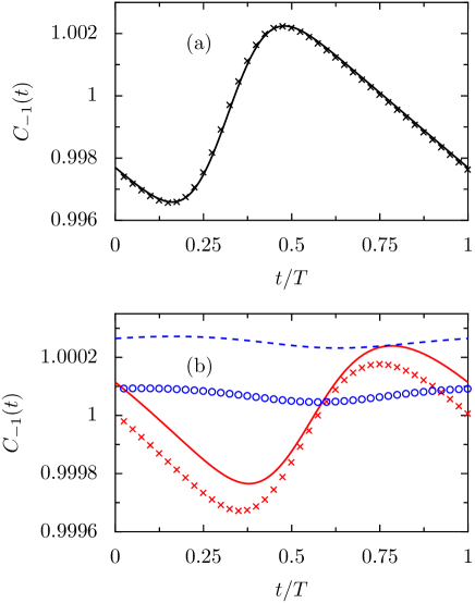
Figure 13: The comparison of the approximations II and III for the coefficient $C_{-1}(t)$ shows perfect agreement for driving frequencies $\Omega\leq 0.1$, see panel (a) for $\Omega=0.1$ (method II: crosses, method III: solid line). Relatively small but on the scale of the variability apparent deviations between the methods become visible for $\Omega=0.5$ (red, method II: crosses, method III: solid line) and $\Omega=1$ (blue, method II: circles, method III: dashed line) in panel (b). The remaining parameters in both panels are with $A=0.1$, $D=2.5\times 10^{-2}$ the same as in Fig. 8.

The relative deviation between the coefficients $C_{\pm}(t)$ resulting from the approximations II and III were smaller than $5\times 10^{-4}$ in all investigated cases. Clear deviations are visible only on the scale of the variability of the coefficients for frequencies $\Omega>0.1$, see Fig 13.

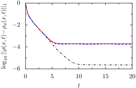
Figure 14: After a short relaxation time, the decadic logarithm of the $L_{1}$ distance between the numerical solution of the Fokker-Planck equation and the proposed asymptotic form (78) reveals a perfect agreement with $\rho_{\text{III}}$ within the expected numerical precision of the solution of the Fokker-Planck equation (black, dash-dotted line). In the case of the first method (red, solid line) which uses the decoration with the current carrying densities, the absorbing boundary conditions at one of the metastable states leads to a larger distance from the asymptotic pdf. This also happens with method II (blue, dashed line) which is based on the estimate (76) of the coefficients $C_{\pm 1}(t)$ which lacks a rigorous foundation. Yet the observed agreement is very good even for rather fast driving with the frequency $\Omega=1$. The remaining parameters are with $A=0.1$, $D=2.5\times 10^{-2}$ the same as in Fig. 8.

The distances between the numerically exact solution of the Fokker-Planck equation and the pdfs obtained from the decoration of the metastable states according to the three methods described above are displayed in Fig. 14. In all cases, after a short initial time, an exponential relaxation sets in until the pdfs obtained from method II as well as from the decoration with the current carrying pdfs saturate at a distance of the order of $2\times 10^{-4}$. For method III it does so at the smaller distance of $2\times 10^{{-6}}$. This is a clear indication that the asymptotic pdf is indeed of the form of eq. (78). This hence corroborates a basic assumption of our work about the structure of the pdf at large times.

6 Summary

We investigated the large time stochastic dynamics of periodically driven systems with metastable states governed by a Fokker-Planck equation. On time scales larger than the typical deterministic time scale this dynamics can be completely characterized by the localizing functions, the $\alpha$-specific pdfs and the conditional occupation probabilities of the metastable states. The latter are solutions of a Markovian master equation with time-dependent rates. These rates can be expressed in terms of the localizing functions and the $\alpha$-specific pdfs, see eq. (24).

Using the Floquet representation of the conditional pdf in the large time limit we obtained coupled equations of motion for the $\alpha$-specific densities and an adjoint set of equations for the localizing functions. Most interestingly, these equations of motion can be interpreted in the spirit of Farkas’ [30] and Kramers’ [31] idea to construct a flux carrying stationary solution by imposing convenient sources and sinks. To each $\alpha$-specific density an $\alpha$-process can be assigned that evolves according to the same dynamical laws as the original process with the only difference that it can instantly be translocated in state space. These translocations are governed by sinks and sources that cause a sudden death of an $\alpha$-process, say, at a point ${\mathbf{x}}$ and the instant resurrection of the same process at a different point ${\mathbf{y}}$ in state space. The sinks are determined by the sum of transition rates out of the metastable state $\alpha$ multiplied by those $\beta$ specific pdfs corresponding to states that can directly be reached from $\alpha$. The source is given by the total rate to leave state $\alpha$ multiplied by its specific pdf. In this way the conservation of probability of each specific pdf is guaranteed. Due to the resulting intricate coupling and the dependence on the unknown rates, an exact solution is difficult to construct and one must rely on approximate methods to solve this set of equations of motion for the $\alpha$-specific pdfs.

An efficient way of approximation is based on the fact that at weak noise the $\alpha$-specific pdfs are expected to be strongly localized in the region of the according metastable state. This allows one to effectively decouple the equations for the $\alpha$-specific pdfs (as well as those for the localizing functions) and to calculate a current carrying pdf in the presence of sharply absorbing states. The rates of all transitions leaving the considered metastable state can then be calculated by means of a flux-over-population expression [30, 31, 32]. In contrast to the case without time-dependent driving it is important to calculate the probability flux flowing directly into the final metastable state. In the time independent case this flux is the same through all hypersurfaces in state space separating the initial from the final metastable state. In the presence of periodic driving the total flux through a hypersurface in general depends both on time and on the location of the chosen hypersurface. The proper rate therefore must be determined from the probability flux flowing directly into the final metastable state.

We illustrated our theory with the example of a periodically driven bistable Brownian oscillator. In contrast to a slowly driven bistable oscillator, at finite frequencies bistability extends to larger amplitudes of the driving force. We found that the flux-over-population method based on the $\alpha$-specific pdf with an absorbing boundary at the final metastable state requires a much lesser computational effort than the direct application of the Floquet approach. In the former case the solution of the Fokker-Planck equation with the appropriate boundary conditions converges on the order of the deterministic time scale, whereas for the second method the convergence of the Floquet functions is only reached after several transitions between the metastable states have taken place on average.

We note that based on the absorbing boundary approximation the transition rates can also be determined by means of numerical simulations of the Langevin equations of the considered Fokker-Planck process [17, 18, 19].

We finally tested the crucial assumption of our theory saying that the probability density resulting as the large time solution of the Fokker-Planck equation can be represented as the product of the probabilities of the metastable states decorated by the specific pdfs. The time dependence of the probabilities of the metastable states was obtained from the solution of the master equation with the numerically determined flux-over-population rates. The specific pdfs obtained by the absorbing boundary approximation already lead to an excellent agreement with the numerically exact solution of the Fokker-Planck equation on time scales larger than a few characteristic deterministic times. A more elaborate calculation of the specific pdfs in terms of Floquet eigenfunctions of the Fokker-Planck operator led to a further improvement of the agreement by two orders of magnitude confirming our assumption.

References

- [1] Pollak, E., J. Chem. Phys. 85 (1986) 865.
- [2] Pollak, E., H. Grabert, P. Hänggi, J. Chem. Phys. 91 (1989) 4073.
- [3] Hänggi, P., P. Talkner, M. Borkovec, Rev. Mod. Phys. 62 (1990) 251.
- [4] Pollak, E., P. Talkner, Chaos 15 (2005) 026116.
- [5] Jung, P., P. Hänggi, Phys. Rev. A 41 (1990) 2977.
- [6] Jung, P., P. Hänggi, Phys. Rev. A 44 (1991) 8032.
- [7] Jung, P., Phys. Rep. 234 (1993) 175 .
- [8] Gammaitoni, L., P. Hänggi, P. Jung, F. Marchesoni, Rev. Mod. Phys. 70 (1998) 223.
- [9] Astumian, R.D., P. Hänggi, Physics Today 55 (No. 11) (2002) 33.
- [10] Reimann, P., Phys. Rep. 361 (2002) 57.
- [11] Hänggi, P., F. Marchesoni, Rev. Mod. Phys. 81 (2009) 387.
- [12] Machura, L., M. Kostur, P. Talkner, J. Łuczka, P. Hänggi, Phys. Rev. E 98 (2007) 040601.
- [13] R. Zwanzig, Nonequilibrium Statistical Mechanics, Oxford University Press, Oxford 2001.
- [14] Pollak, E., P. Pechukas, J. Chem. Phys. 69 (1978) 1218.
- [15] Talkner, P., New J. Phys. 1 (1999) 4.
- [16] Talkner, P., J. Łuczka, Phys. Rev. E 69 (2004) 046109.
- [17] Talkner, P., L. Machura, M. Schindler, P. Hänggi, J. Łuczka, New J. Phys. 7 (2004) 14.
- [18] Schindler, M., P. Talkner, P. Hänggi, Phys. Rev. Lett. 93 (2004) 048102.
- [19] Schindler, M., P. Talkner, P. Hänggi, Physica A 351 (2005) 40.
- [20] Doering, C.R., J.C. Gadoua, Phys. Rev. Lett. 69 (1992) 2318.
- [21] Pechukas, P., P. Hänggi, Phys. Rev. Lett. 73 (1994) 2772.
- [22] Luchinsky, D.G. , P.V.E. McClintock, M.I. Dykman, Rep. Prog. Phys. 61 (1998) 889.
- [23] Lehmann, J., P. Reimann, P. Hänggi, Phys. Rev. Lett. 84 (2001) 1639.
- [24] Lehmann, J., P. Reimann, P. Hänggi, phys. stat. sol. (b) 237 (2003) 53.
- [25] Hänggi, H. Thomas, Phys. Rep. 88 (1982) 207.
- [26] H. Risken, The Fokker-Planck Equation, Springer-Verlag, Berlin 1984.
- [27] Talkner, P., Ann. Phys. (Leipzig) 9 (2000) 741.
- [28] The Floquet eigenvalue is non-degenerate if the diffusion matrix is non-singular. There are also processes with singular diffusion matrices such as for Fokker-Planck operators of the Klein-Kramers type for which is still non-degenerate.
- [29] N.G. van Kampen, Stochastic Processes in Physics and Chemistry, North Holland, Amsterdam, 1992.
- [30] Farkas, L., Z. Phys. Chem. (Leipzig) 125 (1927) 236.
- [31] Kramers, H.A., Physica (Utrecht) 7 (1940) 284.
- [32] Reimann, P., G.J. Schmid, P. Hänggi, Phys. Rev. E 60 (1999) R1.
- [33] Langer, J.S., Ann. Phys., (N.Y.) 54 (1969) 258.
- [34] Berzis, M. P.M. Dew, ACM Trans. Math. Software 17 (1991) 178.