Coarse Grained Simulations of a Small Peptide: Effects of Finite Damping and Hydrodynamic Interactions

Abstract

In the coarse grained Brownian Dynamics simulation method the many solvent molecules are replaced by random thermal kicks and an effective friction acting on the particles of interest. For Brownian Dynamics the friction has to be so strong that the particles’ velocities are damped much faster than the duration of an integration timestep. Here we show that this conceptual limit can be dropped with an analytic integration of the equations of damped motion. In the resulting Langevin integration scheme our recently proposed approximate form of the hydrodynamic interactions between the particles can be incorparated conveniently, leading to a fast multi-particle propagation scheme, which captures more of the short-time and short-range solvent effects than standard BD. Comparing the dynamics of a bead-spring model of a short peptide, we recommend to run simulations of small biological molecules with the Langevin type finite damping and to include the hydrodynamic interactions.

I Introduction

For the simulation of microscopic particles in a solvent, Brownian Dynamics (BD) has become a work horse technique, which is routinely applied to study, e.g., the properties of colloidal suspensions PHI88 ; LAD90 ; GOR04 , the dynamics of polymers LIU03 ; BEA00b ; SZY07 ; EMP08 , or the association of biological proteins GAB02 ; MIN05 ; SPA06 ; DLU08 . Einstein’s seminal explanation of the random thermal motion of microscopic objects in a solvent EIN05 , which had been discovered earlier by Robert Brown, is based on the assumption that the solvent molecules are so much smaller than the interesting objects that they can be replaced by a continuous solvent, which then modifies the motion of the much larger Brownian particles in three major ways. First, the kinetic energy of the large particles is dissipated via the viscosity of the solvent. Second, the thermal motion of the solvent molecules is replaced by random kicks to the observed particles. These two contributions effectively form a thermostat. Third, the direct interactions like Coulomb or short range van-der-Waals interactions are modified by the solvent. With these three modifications, the problem of solving Newton’s equations of motion for very many particles with well-defined position-dependent interaction potentials is replaced by solving a few-body problem with more complex interactions, a velocity-dependent dissipation, and an additional noise term. This level of approximation is often referred to as Langevin Dynamics (LD), whereas Brownian Dynamics involves the additional approximation that only ”long” time intervals are considered DHO96 . Then, due to the damping of the particle velocities, all information about the momentum is lost between two subsequent observations. This is called the overdamped regime.

Obviously, the central criterion whether BD is an adequate simulation method, is that the solvent molecules are indeed much faster—or that the Brownian particles are much larger and thus slower than a water molecule with its effective diameter of about 1.5 Å. For colloidal particles with diameters on the micron scale this separation of scales is a good approximation, but for the much smaller biological proteins with diameters of a few nanometers it is already questionable. This becomes even more pronounced, when this coarse grained method is applied to the internal dynamics of proteins.

In addition to the thermostat effect, the solvent also mediates a mechanical coupling between the observable particles, the so called hydrodynamic interactions (HI). The resulting correlations in the particle velocities may have striking effects on the folding behavior of proteins as shown recently FRE09 .

Here, we investigate the effects of the approximations outlined above. For a bead-spring representation of a short peptide we compare plain BD simulations to BD simulations with HI included and also to LD simulations both with and without HI to see how the simulated dynamics of very small particles is influenced by the non-negligible relaxation times and how the hydrodynamic coupling between the beads affects the overall dynamics. In the next section we introduce our implementation of the LD and BD algorithms and how hydrodynamic interactions can be incorporated efficiently. There we also explain the coarse graining procedure used to set up the bead-spring model of the peptide. The results then show how the different approximations influence the dynamic behavior of the model peptide.

II Methods

II.1 Langevin and Brownian Propagation

For the following it is convenient to formulate the Brownian and the Langevin propagation algorithms with effective forces instead of directly using displacements as in the original BD scheme of Ermak and McCammon ERM78 . For this, we start from Newton’s equations of motion for the complete system including all solvent molecules. Obviously, the particle masses $m_{i}$ can be taken as constant such that the change of the momenta $p_{i}$ can be expressed as a change of the velocities $v_{i}$ due to the sums $F_{i}$ of all pairwise position-dependent forces.

$$\frac{dp_{i}}{dt}=m_{i}\frac{dv_{i}}{dt}=F_{i}=\sum_{k\neq i}F(r_{ik})$$ (1)

The dimensionality of this system of equations can be greatly reduced by assuming that the solvent molecules are very small. Then their masses are very small and they move so fast that their effect on the slower degrees of freedom of the interesting particles can be treated as a mean-field heat bath consisting of a dissipative friction term plus a random driving EIN05 . For a spherical particle, the phenomenological friction constant $\gamma$ can be calculated via the Stokes-Einstein relation from the hydrodynamic radius $a$ of the particle and the macroscopic bulk viscosity $\eta$ of the solvent as $\gamma=6\pi\eta a$ DHO96 . Due to the random nature of the driving kicks from the solvent molecules, these kicks are characterized via the statistical measures of a vanishing average and a finite covariance of the resulting displacements $R_{i}(\delta t)$:

$$\langle R_{i}\rangle=0\quad\mbox{and}\quad\langle R_{i}R_{k}\rangle=2D_{ik}\delta t$$ (2)

For the diagonal terms with $i=k$ the diffusion coefficient $D_{ii}=k_{B}T/\gamma_{i}$ gives the ratio between the solvent induced thermal energy $k_{B}T$ and the also solvent mediated dissipation. For the off-diagonal terms, $D_{ik}$ describes the hydrodynamic coupling due to the displaced solvent.

To determine the random displacements $R_{i}$ from the covariance (2), one essentially has to take the square root of the diffusion matrix FIX81 . Due to the high numerical cost associated with this step, the hydrodynamic coupling was often neglected in BD simulations by setting the off-diagonal entries $D_{ik}=0$. It was only recently that we could show how this expensive matrix factorization can be approximated by a sum of two-body contributions and the correlated random displacements can be expressed via effective random forces GEY09 $f_{i}^{eff}$, leading to the same $\mathcal{O}(N^{2})$ runtime scaling as for the pairwise direct interactions $F_{ik}$.

To arrive at a formulation of the equation of motion with the implicit solvent which is convenient for numerical propagation, we start from (1) with the total force $F=F_{ext}+f$, which is the sum of the external forces $F_{ext}$ and the random kicks $f$:

$$\frac{dv}{dt}=\frac{1}{m}(F-\gamma v)$$ (3)

For simplicity, we omit the coordinate index $i$ for the following. This equation of motion can be integrated analytically over one timestep of length $\Delta t$, which must be so small that the configuration dependent forces remain essentially constant BEA00a . Due to the linear Stokes friction, we can use the average $f(\Delta t)$ of the random kicks. With the initial velocity $v_{0}$, $v(\Delta t)$ at the end of the timestep is then

$$v(\Delta t)=\frac{F}{\gamma}+\left(v_{0}-\frac{F}{\gamma}\right)\mbox{e}^{-\frac{\gamma\Delta t}{m}}$$ (4)

This equation can be integrated once more to give the displacement $\Delta x(\Delta t)$ during $\Delta t$:

$$\Delta x(\Delta t)=\frac{F}{\gamma}\Delta t-\frac{m}{\gamma}\left(\frac{F}{\gamma}-v_{0}\right)\left(1-\mbox{e}^{-\frac{\gamma\Delta t}{m}}\right)$$ (5)

From these equations the conventional BD propagation algorithm is obtained by going to the overdamped regime where $\Delta t\gg\tau_{rel}$, i.e., only timesteps $\Delta t$ are considered that are much longer than the velocity relaxation time $\tau_{rel}=m/\gamma$. Then $v_{0}$ can be neglected and the displacement simplifies to

$$\Delta x(\Delta t)=\frac{F}{\gamma}\Delta t=\frac{D_{0}}{k_{B}T}F\,\Delta t,$$ (6)

which can also be expressed with the diffusion constant $D_{0}=k_{B}T/\gamma$ of the particle.

For the rotational motion, analogous equations are used where position $x$ and velocity $v$ are replaced by a rotation angle and an angular velocity, and torques instead of the forces $F$ act on moments of inertia.

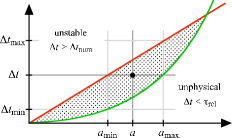
Figure 1: Range of admissible timesteps $\Delta t$ between the inaccurate and the unphysical regimes of a BD simulation vs. particle radius $a$. The lower green line denotes the conceptual limit according to $\Delta t\gg\tau_{rel}\propto a^{2}$. The upper red limit indicates that the maximal timestep for a numerically stable propagation increases only $\propto a$. Consequently, for any $\Delta t$ there is a minimal particle size $a_{min}$, for which the propagation becomes unstable, and a maximal $a_{max}$, for which the assumption of overdamped motion is not valid anymore. For further explanations see text.

The Langevin equations (4) and (5) look much more complex than the Brownian propagator (6), but for practical applications the main effort is to determine the forces and torques acting on each of the particles. Thus, keeping track of the velocity only incurs a negligibly small additional overhead for the benefit that one has not to make sure that the conceptual constraint of BD, $\Delta t\gg\tau_{rel}$, is fulfilled. It is actually quite easy to find simulation scenarios where these BD requirements cannot be fulfilled for all particles simultaneously. This can be seen from the following estimate of the two limits for $\Delta t$. The first is that $\Delta t\gg\tau_{rel}=m/\gamma$. For typical colloidal particles or biological polymers, the mass $m=\frac{4\pi}{3}\rho a^{3}$ is proportional to the volume and thus scales $\propto a^{3}$ with the radius $a$. From the Stokes-Einstein relation we get $\gamma=6\pi\eta a\propto a$, thus $\tau_{rel}=\frac{2}{9}\frac{\rho a^{2}}{\eta}$ increases quadratically with $a$. On the other hand, $\Delta t$ has to be small enough for numerical reasons to keep the typical displacements $\Delta x(\Delta t)\ll\Delta x_{max}$, where $\Delta x_{max}$ is a typical potential well extensions or the dimensions of the smallest particles. According to (6) this upper limit scales $\propto a$. In a simulation where all particles have the same size, usually a $\Delta t$ can be found, which fulfills both requirements. However, when particles of different sizes are considered, a timestep which allows for a stable propagation of the small particles may be much shorter than $\tau_{rel}$ for the largest particles, while a $\Delta t$ that ensures the overdamped regime for the larger particles most likely leads to numerical instabilities. This problem is sketched in figure 1, where the green line denotes the lower limit from the overdamped regime and the red line the upper numerical stability margin. The dotted area between these two limits is the area of permissible timesteps. For a fixed $a$ there is a certain region $[\Delta t_{min},\Delta t_{max}]$ for $\Delta t$ to choose from, but when particles of different sizes are used in the same simulation, then for a given timestep $\Delta t$ there is only a range of particle sizes $[a_{min},a_{max}]$ which can be propagated reliably within the assumption of Brownian Dynamics.

A few numbers highlight this problem. With a typical protein density of $\rho=1.1\rho_{H_{2}O}$ and $\rho/\eta=1.23$ ps/nm² we find that a protein of $a$ = 5 nm radius has $\tau_{rel}=6.8$ ps. The small electron carrier cytochrome $c_{2}$ with $a=1.67$ nm has only $\tau_{rel}=0.76$ ps and an ion with an effective hydrodynamic radius of 0.2 nm looses its velocity already within $\tau_{rel}=0.01$ ps. In a simulation with cytochrome $c_{2}$ and ions, based on practical experience, a timestep of $\Delta t=1$ ps still yields a stable propagation of the fast ions. While the ions are clearly in the overdamped regime, this assumption is at least questionable for the cytochrome $c_{2}$. When one wants to simulate the association of cytochrome $c_{2}$ to larger proteins in the presence of explicitly modelled ions, $\Delta t=1$ ps is clearly too short for a theoretically valid overdamped BD description.

We note that for the analytical integration above we required that the interparticle forces be constant during one timestep. When the underlying interaction potentials are not approximated by constant slopes but one order further by harmonic potentials, the analytical solutions for the motion of a damped harmonic oscillator can be used for the propagator. Though this is not really practical, it allows to distinguish between the strongly damped creeping and the weakly damped ballistic regimes based on the ratio of potential curvature and relaxation time. With this criterion and the parameter values above, only for very short ranged potentials like van-der-Waals interactions the dynamics may come close to the weakly damped ballistic and thus oscillatory regime.

II.2 Including Hydrodynamic Interactions

When one wants to include HI into a Langevin propagation as the one from equations (4) and (5), then there is a conceptual difficulty. The usual Oseen KIR48 or Rotne-Prager-Yamakawa ROT69 ; YAM70 (RPY) hydrodynamic tensors are built with the help of the Faxén theorem FAX22 from the stationary flow fields around spheres moving with constant velocities. In an overdamped BD simulation one can at least assume that the velocities are constant during one timestep and then treat each timestep as a configuration with (temporarily) stationary velocities mimicking these creeping flow conditions. Due to the linear Stokes friction, the velocity does not even occur in the BD propagator (6) and the (constant) forces can directly be converted into displacements.

With hydrodynamic interactions the BD propagator (6) for the $i$th coordinate becomes ERM78

$$\Delta x_{i}(\Delta t)=\sum_{k}\frac{D_{ik}F_{k}}{k_{B}T}\Delta t+R_{i}(\Delta t),$$ (7)

which can be rewritten with a hydrodynamically corrected effective force GEY09 $F_{i}^{eff}=\sum_{k}\frac{D_{ik}}{D_{ii}}F_{k}$:

$$\Delta x_{i}(\Delta t)=\frac{D_{ii}\,\Delta t}{k_{B}T}F_{i}^{eff}+R_{i}(\Delta t)$$ (8)

With the RPY HI tensor, the term taking care of local variations of the diffusion coefficients vanishes and is omitted here (see, e.g., the original derivation by Ermak and McCammon ERM78 ). Recently, we could show GEY09 how the expensive calculation of the correlated random displacements $R_{i}(\Delta t)$ can be approximated efficiently with an ansatz that converts the uncorrelated random forces $f_{i}$ into hydrodynamically corrected effective random forces $f_{i}^{eff}$:

$$R_{i}(\Delta t)=\frac{D_{ii}\Delta t}{k_{B}T}C_{i}\sum_{k}\beta_{ik}\frac{D_{ik}}{D_{ii}}f_{i}=\frac{D_{ii}\Delta t}{k_{B}T}f_{i}^{eff}$$ (9)

With $\beta_{ii}=1$, the normalization factors can be determined from

$$\left(\frac{1}{C_{i}}\right)^{2}=1+\sum_{k\neq i}\beta_{ik}^{2}\frac{D_{ik}^{2}}{D_{ii}D_{kk}}$$ (10)

and the quadratic equation

$$\beta_{ik}=\frac{1-\sqrt{1-[(N-1)\epsilon^{2}-(N-2)\epsilon]}}{(N-1)\epsilon^{2}-(N-2)\epsilon},$$ (11)

where $\epsilon=\langle D_{ik}/D_{ii}\rangle$ is the average normalized off-diagonal entry of the diffusion matrix. Then, the displacements $\Delta x_{i}$ can be calculated efficiently with an overall $\mathcal{O}(N^{2})$ runtime scaling from the hydrodynamically corrected external and random forces and the diagonal entries of the diffusion matrix as

$$\Delta x_{i}(\Delta t)=\frac{D_{ii}\,\Delta t}{k_{B}T}(F_{i}^{eff}+f_{i}^{eff})$$ (12)

We now show how this idea can also be used in an LD description, where the velocities are not constant during a timestep but change from the initial $v_{0}$ to the final $v(\Delta t)$, which is then the new $v_{0}$ for the next step. For this, we need an effective force $\tilde{F}$ which is constant during one timestep and leads to the same total displacement as with the correct propagator. With $\Delta x(\Delta t)=\tilde{F}\Delta t/\gamma$ we find from equation (5)

$$\tilde{F}=\left[1-\frac{m}{\gamma\Delta t}\left(1-\mbox{e}^{-\frac{\gamma\Delta t}{m}}\right)\right]F+\frac{m}{\Delta t}\left(1-\mbox{e}^{-\frac{\gamma\Delta t}{m}}\right)v_{0}.$$ (13)

The new $v_{0}$ for the next timestep is then

$$\tilde{v}_{0}=\exp\left[-\frac{\gamma\Delta t}{m}\right]v_{0}+\frac{1}{\gamma}\left(1-\mbox{e}^{-\frac{\gamma\Delta t}{m}}\right)F\,.$$ (14)

In the actual implementation equations (13) and (14) occur twice, once for the external forces $F_{i}$ and once for the random forces $f_{i}$. From these damping-corrected uncorrelated forces the hydrodynamically correlated forces $\tilde{F}_{i}^{eff}$ and $\tilde{f}_{i}^{eff}$ are then computed as explained above and used to propagate the particles according to equation (12). With this recipe, our recent efficient truncated expansion HI GEY09 can be combined with a Langevin type propagation of Brownian particles, which is conceptually valid even for arbitrarily small timesteps with only negligibly more effort. Most of the prefactors in equations (13) and (14) need only be evaluated once during the simulation setup.

III Results

As a testcase for the propagation schemes outlined above we used a small eleven-residue peptide, which had been used in our group in a recent molecular dynamics (MD) study of the effects of interfacial water layers during peptide-protein association at an SH3 domain AHM08 . The sequence of the peptide is SHRPPPPGHRV using the one-letter codes ALB02 . The four central prolin (P) residues form a rather rigid PP2 helix, the short peptide therefore does not show any folding or unfolding on the considered timescales.

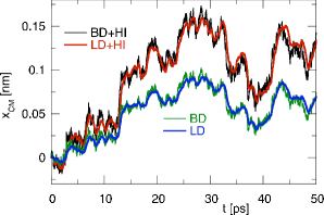
Figure 2: X-component of the trajectory of the peptide CM under the same sequence of random kicks with the different propagation schemes. The inclusion of HI accelerates the CM diffusion and the finite damping of LD smoothes and slightly delays the peptide’s response to the fast thermal kicks without changing the long-time trajectory.

The atomic structure of the peptide was coarse-grained by first placing a van-der-Waals sphere around the C_α atoms of each of the residues. The side chains of the residues, which extended beyond this first sphere, were enclosed in a second (and third) sphere, for which the positions and radii were chosen to reproduce the van-der-Waals surface of the peptide as close as possible. In each residue the effective charges from the PDB structure with $|q|\leq 0.5$ e were kept. Then, the C_α spheres were connected by springs. The diffusion coefficients of the residues were taken from Ma etalMa05 . Running BD simulations of this first setup we determined the resulting mutual center-of-mass (CM) distances for each pair of residues and compared them to the respective distances derived from a 20 ns MD simulation of the peptide in a water box. This reference simulation was performed with the Gromacs package VDS05 using the OPLS all-atom force field JOR96 and the TIP4P water model JOR83 . The MD trajectory consequently includes the finite damping of and the hydrodynamic coupling between the residues. As this first set of springs was not enough to reproduce all distance distributions correctly, additional springs between the CMs of the residues were added and their values optimized manually until a sufficient agreement between the MD results and a standard BD simulation was achieved. With this parametrized bead-spring-model of the peptide we ran BD and LD simulations, each with and without hydrodynamics. In all simulations, a single copy of the peptide was simulated in an unbounded box. The comparison of these four different simulation schemes shows the effects of each of the simplifications.

The calculated relaxation times of the peptide residues range from $\tau_{rel}=32$ fs for the small glycin (G) to 50 fs for the larger arginine (R). For a reliable propagation we used a conservatively estimated small time step $\Delta t=10$ fs in all simulations.

III.1 Center-of-Mass Diffusion

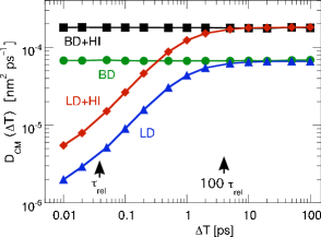
Figure 3: CM diffusion coefficient $D_{CM}=\frac{\langle\Delta r^{2}\rangle}{6\Delta T}$ of the peptide vs. the length of the observation time interval $\Delta T$. The arrow labeled with $\tau_{rel}$ indicates the typical velocity relaxation time of a single residue of $\approx 40$ fs. With LD the long-time value of $D_{CM}$ is obtained only for $\Delta T\geq 100\,\tau_{rel}$. With HI, $D_{CM}$ is increased by a factor of 2.7.

For the diffusion of the CM of the peptide two effects were observed. As for polymers the CM diffusion coefficient $D_{CM}$ was increased when HI was included. This can be well seen in figure 2, which compares the x-component of the CM motion of the peptide obtained with the same sequence of random numbers for the four different propagation schemes. All four curves show the same trends, but the amplitudes from BD+HI and LD+HI are nearly twice as large as without HI. In this plot one can also see that the trajectories with LD are much smoother than with BD due to the finite relaxation time. For both BD with and without HI the power spectrum can be well fitted with a $1/f$ behavior, where the amplitudes with HI are about 60% higher. With LD, however, the amplitudes are the same in the low-frequency range as in the corresponding BD simulations, but fluctuations that occur on timescale shorter than a picosecond are suppressed by about 30% in this one-dimensional representation (data not shown).

Similar conclusions can be drawn from how the CM diffusion coefficient $D_{CM}(\Delta T)$ changes with the length of the observation time step $\Delta T$. Figure 3 gives $D_{CM}=\langle\Delta r^{2}(\Delta T)\rangle/6\Delta T$ for the four different propagation schemes. Here, for the same trajectory, which was simulated at a timestep $\Delta t=10$ fs, the observation window $\Delta T$ was varied at which the CM displacements $\Delta\vec{r}(\Delta T)$ were obtained. As expected, the BD simulations have no implicit time scale and, consequently, give the same $D_{CM}$ for any $\Delta T$. The creeping flow HI used here accelerates the diffusive motion without introducing a timescale of its own and $D_{CM}$ is about 2.7 times larger with hydrodynamics than without. For long observation intervals $\Delta T>10$ ps, the LD propagation reproduces the respective BD values for $D_{CM}$, whereas in the ballistic short time regime $D_{CM}$ increases linearly with $\Delta T$. The relaxation times of the individual residues are in the range $\tau_{rel}=32\ldots 50$ fs, which is indicated in figure 3. However, it takes about two orders of magnitude longer, until $D_{CM}$ from the LD propagation reaches the timescale-free BD value.

III.2 Orientational Relaxation

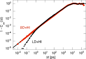
Figure 4: Orientational relaxation of the end-to-end vector $R_{ee}$ as seen from the autocorrelation $C_{ee}$ from BD+HI (red points) and LD+HI simulations (black squares). The solid line indicates the fit to a stretched exponential as explained in the text.

As shown above, the inclusion of HI accelerates the collective CM diffusion. This is accompanied by a slowdown of the internal dynamics. For bead-spring polymers this can, e.g., be seen in a prolonged correlation of the end-to-end vector $\vec{R}_{ee}$ pointing from the first to the last monomer. The peptide used here is too short and not flexible enough to show pronounced differences in the relaxation of $\vec{R}_{ee}$ whether HI are included or not. Nevertheless, the effects of the finite damping can be seen in the autocorrelation $C_{ee}(\Delta t)=\langle\hat{R}_{ee}(t)\hat{R}_{ee}(t+\Delta t)\rangle$, which is plotted in figure 4 as $1-C_{ee}(\Delta t)$. For both BD and BD+HI, $C_{ee}$ fits well to a stretched exponential

$$C_{ee}(\Delta t)=\exp\left[-\left(\Delta t/\tau\right)^{\alpha}\right]$$ (15)

with $\tau$ = 4.1 ns and $\alpha=0.95$. With the LD propagation, the dynamics on timescales shorter than a few picoseconds is slowed down both with and without HI. Correspondingly, in figure 4, $1-C_{ee}$ from the Langevin simulation is smaller than with the overdamped Brownian propagation for short time intervals, while for longer intervals the same exponential decay is observed.

III.3 Internal Dynamics

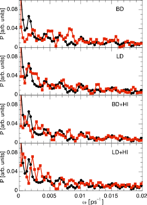
Figure 5: Comparison of the power spectra for the dynamics of the CM distance between the first and the last residue with the different propagation schemes. In all four panels the black data (points) are from the MD simulation and the red (squares) from the respective coarse grained method.

The bonds of the coarse-grained representation of the peptide had been parametrized against the stationary distance distributions without considering the actual dynamics, which are also influenced by the residue masses and the damping. Consequently, the dynamics will have different temporal signatures with the different propagation schemes. Figure 5 shows the power spectrum of the distance between the first and the last bond for the four integration schemes in comparison to the power spectrum extracted from the MD trajectory. These power spectra are typical for the distances between residues located on opposite ends of the peptide.

As seen in figure 5, the first four peaks between 0.002 ps^-1 and 0.01 ps^-1 are present in the LD result and can be recognized in the LD+HI spectrum. BD and BD+HI are damped too fast. Consequently, no real peak structure can be identified above the strongly fluctuating background. For the other distances between residues on opposite ends of the peptide, a similar trend is found.

These spectra now could be further improved by optimizing the effective masses of the residues. However, already these results with the raw textbook-masses demonstrate that the short-time dynamics on the picosecond timescale are better reproduced with the finitely damped Langevin algorithm.

III.4 Numerical Stability and Runtime

The first test had been to compare the distance distributions between the CMs of the residues for all four simulation schemes. As expected, for these static measures no differences beyond the statistical uncertainties were found. Getting the same positions and widths with LD as with BD shows that the velocity relaxation occurs faster than one oscillation period in the interparticle potentials even for the rather hard springs that had to be used along the peptide backbone between the C_α atoms. Otherwise one would expect a widening of the distance distributions and, in the extreme case, a bimodal density as in a classical weakly damped oscillator.

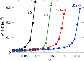
Figure 6: Variance $\sigma^{2}$ of the distance distribution of the bond between residues 5 and 6 vs. the simulation timestep $\Delta t$ for the four propagation schemes.

The stability of each integration scheme was then tested via the variances of the distance distributions for the hard springs, i.e., those distributions which have a small variance. Figure 6 shows the representative behavior for the distance between the fifth and the sixth residue, which are both part of the stiff PP2 helix in the central part of the peptide. With BD alone, timesteps up to 0.05 ps would have been okay, whereas the viscous damping due to HI allows for three times longer timesteps. The same trend is observed for LD, which itself is already more stable than BD because of the damping at high frequencies.

The respective runtimes for 100000 timesteps on a 2.8 GHz Pentium 4 CPU were 18.9 s for BD, 24.2 s for BD+HI, 19.5 s for LD, and 24.5 s for LD+HI. As explained above, keeping track of the velocity in the LD propagation only adds a minimal cost which already pays off when only the numerical stability is taken into account and considerations about the regime of damping are ignored. In this small peptide with its 35 effective charges and 38 bonds, the hydrodynamic interactions between the eleven residues only add a manageable 25% to the total runtime, whereby the direct interactions and the hydrodynamic coupling have the same $\mathcal{O}(N^{2})$ runtime scaling.

IV Summary and Conclusions

In this publication we investigated the effects of a finite damping and of hydrodynamic interactions in Brownian dynamics simulations of a small biological peptide.

Integrating Newton’s equations of motion with a continuous viscous solvent over one timestep, we arrived at a Langevin type integration scheme which allows for the inclusion of our recently introduced efficient approximation for the hydrodynamic coupling GEY09 . With a fast damping this Langevin scheme reduces to the conventional BD algorithm of Ermak and McCammon ERM78 . Due to the analytic integration for one timestep the Langevin propagator is about as fast numerically as the simple BD integration, but does not have the conceptual limitation that the timestep $\Delta t$ has to be much longer than the velocity relaxation time $\tau_{rel}$. This issue arises especially in simulations of proteins of different sizes, because there $\Delta t$ may be too close to $\tau_{rel}$ for the larger proteins, while for the smaller, faster proteins $\Delta t$ is already too long for a stable propagation. With the LD propagator, the length of $\Delta t$ is only limited by numerical accuracy and stability considerations. Actually, our test showed that only when $\Delta t$ is at least two orders of magnitude longer than $\tau_{rel}$, the finite damping may safely be neglected. For practical applications such a long integration timestep is nearly never feasible.

Comparing the dynamics of a small peptide from our coarse grained BD and LD simulations to an atomistic molecular dynamics trajectory, we found that the distance distributions between the residues of the peptide can be reproduced with a bead-spring model with either propagation technique and the same force constants. However, when the dynamics of the relative motions are compared, LD with its more realistic finite damping gives an overall better agreement of the internal dynamics.

For the short and rather stiff peptide investigated here, the influence of hydrodynamic interactions on the internal motion was small. The center-of-mass motion, however, became faster by nearly a factor of three. Compared to a plain BD simulation, the slightly delayed orientational motion with the LD scheme together with the faster translation due to the HI may change the microscopic dynamics during, for example, the association of two proteins or the binding of a small peptide to a larger protein. At close encounter the smoothed motion with LD may then further modify the obtained association and dissociation rates towards a more stable bound state. From a conceptual point of view we therefore recommend to include hydrodynamics and to use a Langevin propagation scheme for coarse grained protein simulations.

From a numerical point of view, we find no difference in runtime for BD vs. LD and a moderate increase in runtime of about 30% for adding our approximate hydrodynamics with its $\mathcal{O}(N^{2})$ runtime scaling. The coarse grained model of the peptide had about six times as many effective charges on the individual residues than there were effective spheres for the hydrodynamics. For peptide or protein models with a similar ratio of the numbers of the simple Coulomb compared to the more expensive hydrodynamic interactions, the runtime cost incurred by HI will be similar.

The finitely damped LD propagation was also more stable numerically, i.e., one could use longer integration timesteps than with the overdamped BD algorithm. The numerical stability of both the BD and the LD schemes further increased with the viscous damping due to the HI. Actually, the longer timesteps that could be used with LD and HI more than compensated for the increased runtime.

Here we used a simple peptide to demonstrate that coarse grained simulation methods need not stop at the level of Einstein’s formulation of Brownian diffusion but that they can also be used very efficiently for much smaller systems, which are usually considered the realm of atomistic simulations or partially coarsened methods, where a few atoms each are summarized into one pseudo atom MAR04 ; GUI06 . The main difference, which makes fine-grained BD and LD simulations so much faster than the coarse grained versions of all-atom descriptions is that the very many solvent molecules do not have to be treated explicitly.

Summarizing we could show that the LD+HI simulation scheme, which includes more of the mechanically induced solvent effects than the conventional BD algorithm, can be formulated and implemented efficiently. Consequently, we are looking forward to applying the methods presented here to larger and more realistic systems in the near future. Potential applications will be the investigation of association funnels of peptide-protein encounter SPA06 ; AHM08 , the folding of coarse grained proteins FRE09 , and dense many-particle scenarios like the cytosol inside a biological cell.

The LD and HI algorithms presented here have been implemented in a general purpose multi-particle BD/LD simulation library, which will be available from the corresponding author free of charge for academic use.

V Acknowledgements

We thank Ahmad Mazen for the post-processed atomic coordinates and the molecular dynamics trajectory of the simulated peptide. This work was funded by the Deutsche Forschungsgemeinschaft through the Graduiertenkolleg 1276/1.

References

- (1) R. J. Phillips, J. F. Brady and G. Bossis, Phys. Fluids 31 3462 (1988)
- (2) A. J. C. Ladd, J. Chem. Phys. 93 3484 (1990)
- (3) C. Gorba, T. Geyer, and V. Helms, J. Chem. Phys. 121, 457 (2004)
- (4) B. Liu and B. Dünweg, J. Chem. Phys. 118, 8061 (2003)
- (5) D. A. Beard and T. Schlick, J. Chem. Phys. 112 7323 (2000)
- (6) P. Szymczak and M. Cieplak, J. Chem. Phys. 127, 155106 (2007)
- (7) A. Emperador, O. Carrillo, M. Rueda and M. Orozco, Biophys. J. 95 2127 (2008)
- (8) D. D. J. Minh, J. M. Bui, C. Chang, T. Jain, J. M. J. Swanson and A. J. McCammon, Biophys. J. 89 L25 (2005)
- (9) R. R. Gabdoulline and R. C. Wade, Curr. Op. Struc. Biol. 12, 204 (2002)
- (10) A. Spaar, C. Dammer, R. R. Gabdoulline, R. C. Wade, and V. Helms, Biophys. J. 90, 1913 (2006)
- (11) M. Dlugosz, J. A. Antosiewicz, and J. Trylska, J. Chem. Theory Comput. 4, 549 (2008)
- (12) A. Einstein, Ann. d. Physik 17, 549 (1905)
- (13) J. K. G. Dhont, An Introduction to Dynamics of Colloids (Elsevier, Amsterdam, 1996)
- (14) T. Frembgen-Kesner and A. H. Elcock J. Chem. Theory Comput. 5 242 (2009)
- (15) D. L. Ermak and J. A. McCammon, J. Chem. Phys. 69, 1352 (1978)
- (16) M. Fixman, Macromolecules 14 1710 (1981)
- (17) T. Geyer and U. Winter, J. Chem. Phys. 130 114905 (2009)
- (18) D. A. Beard and T. Schlick, J. Chem. Phys. 112 7313 (2000)
- (19) J. G. Kirkwood and J. Riseman, J. Chem. Phys. 16, 565 (1948)
- (20) J. Rotne and S. Prager, J. Chem. Phys. 50, 4831 (1969)
- (21) H. Yamakawa, J. Chem. Phys. 53, 436 (1970)
- (22) H. Faxen, Ann. d. Phys. 373 89 (1922)
- (23) M. Ahmad, W. Gu and V. Helms, Angew. Chem. Int. Ed. 47 7626 (2008)
- (24) B. Alberts, A. Johnson, J. Lewis, M. Raff, K. Roberts and P. Walter, Molecular Biology of the Cell, 4th Ed. (Garland Science, New York, Amsterdam, 2002)
- (25) D. Van Der Spoel, E. Lindahl, B. Hess, G. Groenhof, A. E. Mark and H. J. Berendsen, J. Comput. Chem. 26, 1701 (2005)
- (26) W. L. Jorgensen, D. S. Maxwell and J. Tirado-Rives, J. Am. Chem. Soc. 118, 11225 (1996)
- (27) W. L. Jorgensen, J. Chandrasekhar, J. D. Madura, R. W. Impey and M. L. Klein, J. Chem. Phys. 79, 926 (1983)
- (28) Y. Ma, C. Zhu, P. Ma and K. T. Yu, J. Chem. End. Data 50, 1192 (2005)
- (29) S. J. Marrink, A. H. de Vries and A. E. Mark, J. Phys. Chem. B 108 750 (2004)
- (30) G. Guigas and M. Weiss, Biophys. J. 91 2393 (2006)