A canonical form for Projected Entangled Pair States and applications

D. Pérez-García1, M. Sanz2, C. E. González-Guillén1, M. M. Wolf3, J. I. Cirac2 1Dpto. Análisis Matemático and IMI, Universidad Complutense de Madrid, 28040 Madrid, Spain
2Max-Planck-Institut für Quantenoptik, Hans-Kopfermann-Str. 1, 85748 Garching, Germany
3Niels Bohr Institute, Blegdamsvej 17, 2100 Copenhagen, Denmark
Abstract

We show that two different tensors defining the same translational invariant injective Projected Entangled Pair State (PEPS) in a square lattice must be the same up to a trivial gauge freedom. This allows us to characterize the existence of any local or spatial symmetry in the state. As an application of these results we prove that a SU(2)𝑆𝑈2SU(2) invariant PEPS with half-integer spin cannot be injective, which can be seen as a Lieb-Shultz-Mattis theorem in this context. We also give the natural generalization for U(1)𝑈1U(1) symmetry in the spirit of Oshikawa-Yamanaka-Affleck, and show that a PEPS with Wilson loops cannot be injective.

I Introduction

The isolation of Projected Entangled Pair States (PEPS) AKLT88 ; PEPS as an appropriate representation for ground states of 2D local Hamiltonians Hastings turns the problem of understanding 2D quantum many body systems into the question: How can one characterize the different phases of matter in terms of the tensors defining a PEPS?

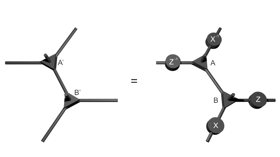
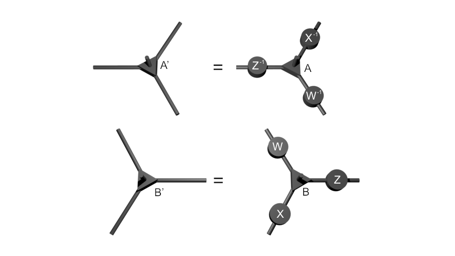
Though there are known examples of PEPS with topological order Verstraete ; Guifre , power law decay of correlations Verstraete , SU(2)𝑆𝑈2SU(2)-symmetry AKLT88 ; Rico , or universal power for measurement based quantum computation Verstraete ; Gross , characterizing these phases has turned out to be a daunting task. In this paper we provide a simple characterization of the existence of symmetries (both local and spatial) as a trivial consequence of the fact, which we call canonical form, that two PEPS describing the same translational invariant state in a square lattice are related by invertible matrices in the virtual spins, as in Fig. 1.

Refer to caption
Figure 1: This is the Canonical Form for PEPS, i.e., the relation that holds between the tensors which define the PEPS when they represent the same state.

This simple characterization illuminates the restrictions that symmetries impose on quantum systems. For instance one can in this context understand the validity of the Lieb-Shultz-Mattis theorem in arbitrary dimensions LSM61 ; HastingsLSM , as well as its U(1)𝑈1U(1) generalization due to Oshikawa, Yamanaka and Affleck OYA97 (originally only in the 1D case). We can also understand why and how three of the main indicators of topological order, namely degeneracy of the ground state, existence of Wilson loops and correction to the area law, are related. Moreover, it has been proven in PWSVC08 that the existence of symmetries in increasing sizes of the system gives the appropriate definition of string order in 2D, overcoming the drawbacks sketched in Anfuso . The importance of string orders in the study of quantum phase transitions, may vaticinate interesting applications in the future along this direction.

Before introducing PEPS formally, we will start with the simpler case of Matrix Product States (MPS), their 1D analogue FNW92 ; PVWC07 . Let us consider a system with periodic boundary conditions of N𝑁N (large but finite number of) sites, each of them with an associate d𝑑d-dimensional Hilbert space. An MPS on this system is defined by a set of D×D𝐷𝐷D\times D matrices {AiD,i=1,,d}formulae-sequencesubscript𝐴𝑖subscript𝐷𝑖1𝑑\{A_{i}\in\mathcal{M}_{D}\,,\,i=1,\ldots,d\} and reads

|ϕA=i1,,iNtr[Ai1AiN]|i1iN.ketsubscriptitalic-ϕ𝐴subscriptsubscript𝑖1subscript𝑖𝑁trdelimited-[]subscript𝐴subscript𝑖1subscript𝐴subscript𝑖𝑁ketsubscript𝑖1subscript𝑖𝑁|\phi_{A}\rangle=\sum_{i_{1},\ldots,i_{N}}{\rm tr}\left[A_{i_{1}}\cdots A_{i_{N}}\right]|i_{1}\cdots i_{N}\rangle\;.

An alternative but equivalent view is the valence bond construction: consider a pair of D𝐷D dimensional ancillary/virtual Hilbert spaces associated to each site and connect every pair of neighboring virtual Hilbert spaces by maximally entangled states (usually called entangled bonds). The MPS is then the result of projecting the virtual Hilbert spaces into the real/physical one by the map 𝒜=iαβAi,αβ|iαβ|𝒜subscript𝑖𝛼𝛽subscript𝐴𝑖𝛼𝛽ket𝑖bra𝛼𝛽\mathcal{A}=\sum_{i\,\alpha\,\beta}A_{i,\alpha\beta}|i\rangle\langle\alpha\beta|.

A key property within MPS theory is called injectivity FNW92 ; PVWC07 and it essentially means that different boundary conditions give rise to different states. Let us formally define it:

Definition 1 (Injectivity).

An MPS |ϕAketsubscriptitalic-ϕ𝐴|\phi_{A}\rangle is injective in a region R𝑅R (whose minimal length we denote by L0subscript𝐿0L_{0}) if the map ΓR(X)=i1,,iL0tr(XAi1AiL0)|i1iL0subscriptΓ𝑅𝑋subscriptsubscript𝑖1subscript𝑖subscript𝐿0tr𝑋subscript𝐴subscript𝑖1subscript𝐴subscript𝑖subscript𝐿0ketsubscript𝑖1subscript𝑖subscript𝐿0\Gamma_{R}(X)=\sum_{i_{1},\ldots,i_{L_{0}}}\operatorname{tr}(XA_{i_{1}}\cdots A_{i_{L_{0}}})|i_{1}\cdots i_{L_{0}}\rangle which associates boundary conditions of R𝑅R to states in R𝑅R is injective. That is, different boundary conditions give rise to different states. An MPS is said to be injective if it is injective for some region R𝑅R.

If we do not take into consideration translational invariance, we can talk about MPS with ‘open boundary conditions’ (OBC). An OBC-MPS is then a state of the form

|Φ=i1,,iNAi1[1]AiN[N]|i1iNketΦsubscriptsubscript𝑖1subscript𝑖𝑁superscriptsubscript𝐴subscript𝑖1delimited-[]1superscriptsubscript𝐴subscript𝑖𝑁delimited-[]𝑁ketsubscript𝑖1subscript𝑖𝑁|\Phi\rangle=\sum_{i_{1},\ldots,i_{N}}A_{i_{1}}^{[1]}\cdots A_{i_{N}}^{[N]}|i_{1}\cdots i_{N}\rangle

where Ai[k]superscriptsubscript𝐴𝑖delimited-[]𝑘A_{i}^{[k]} are Dk×Dk+1subscript𝐷𝑘subscript𝐷𝑘1D_{k}\times D_{k+1} matrices with D1=DN+1=1subscript𝐷1subscript𝐷𝑁11D_{1}=D_{N+1}=1. By taking successive singular value decompositions one can always find a canonical OBC-MPS form of a state Guifre2 ; PVWC07 , which is characterized by the following conditions:

  1. 1.

    iAi[m]Ai[m]=𝟙subscript𝑖subscriptsuperscript𝐴delimited-[]𝑚𝑖subscriptsuperscript𝐴delimited-[]𝑚𝑖1\sum_{i}A^{[m]}_{i}A^{[m]\dagger}_{i}=\mathbbm{1} for all 1mN1𝑚𝑁1\leq m\leq N.

  2. 2.

    iAi[m]Λ[m1]Ai[m]=Λ[m],subscript𝑖subscriptsuperscript𝐴delimited-[]𝑚𝑖superscriptΛdelimited-[]𝑚1subscriptsuperscript𝐴delimited-[]𝑚𝑖superscriptΛdelimited-[]𝑚\sum_{i}A^{[m]\dagger}_{i}\Lambda^{[m-1]}A^{[m]}_{i}=\Lambda^{[m]}, for all 1mN1𝑚𝑁1\leq m\leq N,

  3. 3.

    Λ[0]=Λ[N]=1superscriptΛdelimited-[]0superscriptΛdelimited-[]𝑁1\Lambda^{[0]}=\Lambda^{[N]}=1 and each Λ[m]superscriptΛdelimited-[]𝑚\Lambda^{[m]} is diagonal, positive, full rank and trΛ[m]=1trsuperscriptΛdelimited-[]𝑚1\operatorname{tr}{\Lambda^{[m]}}=1.

PEPS are the natural extension of the MPS beyond the 1D case, where the projection is performed from a larger number of virtual Hilbert spaces depending on the co-ordination number of the lattice (the square lattice, for instance, has four virtual Hilbert spaces). Therefore, the local building blocks are tensors instead of matrices which implies that most calculations become much harder Norbert .

Let us consider an L×N𝐿𝑁L\times N square lattice of spins of dimension d𝑑d. A PEPS consists on a tensor Aldruisubscriptsuperscript𝐴𝑖𝑙𝑑𝑟𝑢A^{i}_{ldru} with 5 indexes: i𝑖i corresponding to the physical spin of dimension d𝑑d and l,d,r,u𝑙𝑑𝑟𝑢l,d,r,u (left, down, right, up) corresponding to four virtual spaces of dimensions (bonds) D1subscript𝐷1D_{1} and D2subscript𝐷2D_{2}, as we did for MPS. The connections between two sites are again performed by means of maximally entangled states |Ω=α|ααketΩsubscript𝛼ket𝛼𝛼|\Omega\rangle=\sum_{\alpha}|\alpha\alpha\rangle. Then, the shape of these states is

|ϕA=i1,,iNL𝒞(Aldrui)|i1iNLketsubscriptitalic-ϕ𝐴subscriptsubscript𝑖1subscript𝑖𝑁𝐿𝒞subscriptsuperscript𝐴𝑖𝑙𝑑𝑟𝑢ketsubscript𝑖1subscript𝑖𝑁𝐿|\phi_{A}\rangle=\sum_{i_{1},\ldots,i_{NL}}\mathcal{C}(A^{i}_{ldru})|i_{1}\ldots i_{NL}\rangle

where 𝒞𝒞\mathcal{C} means the contraction of all tensors Aldruisubscriptsuperscript𝐴𝑖𝑙𝑑𝑟𝑢A^{i}_{ldru} along the square lattice.

Associated to any PEPS |ϕAketsubscriptitalic-ϕ𝐴|\phi_{A}\rangle we can define a parent Hamiltonian HAsubscript𝐻𝐴H_{A} PVWC08 , which is locally defined by the projector onto range(ΓR)\operatorname{range}(\Gamma_{R})^{\perp}. It is clear that the |ϕAketsubscriptitalic-ϕ𝐴|\phi_{A}\rangle is a ground state for HAsubscript𝐻𝐴H_{A} and that it minimizes the energy locally, that is, HAsubscript𝐻𝐴H_{A} is frustration free. In the case of 1D it is proven in FNW92 ; PVWC07 that a MPS is injective if and only if |ϕAketsubscriptitalic-ϕ𝐴|\phi_{A}\rangle is the unique ground state of HAsubscript𝐻𝐴H_{A}.

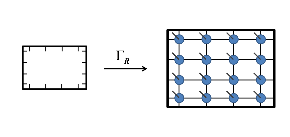
We can define the injectivity property for PEPS in the same way (see Fig 2). That is, the PEPS |ϕAketsubscriptitalic-ϕ𝐴|\phi_{A}\rangle is injective in a region R𝑅R if ΓRsubscriptΓ𝑅\Gamma_{R} is injective. As in the 1D case it is clear that injectivity is a generic condition.
Refer to caption
Figure 2: A PEPS is injective in a region R𝑅R if ΓRsubscriptΓ𝑅\Gamma_{R} is injective, that is, if different boundary conditions give rise to different states in R𝑅R.

In the applications we will give below (Lieb-Shultz-Mattis, Wilson loops), the conclusion will often be that a given PEPS is not injective. What does this mean? As we list below, injectivity is closely related to uniqueness of the ground state of the parent Hamiltonian and to the saturation of the area law for the 0-Renyi entropy.

  1. 1.

    If a PEPS is injective, it is the unique ground state of its parent Hamiltonian PVWC08 .

  2. 2.

    If a PEPS is not-injective for any cylinder-shape region, any local frustration free Hamiltonian for which the given PEPS is a ground state has a degenerate ground space, as long as we grow one of the directions exponentially faster than the other. This is a trivial consequence of the 1D case PVWC07 .

  3. 3.

    The 00-Renyi entropy of the reduced density matrix ρRsubscript𝜌𝑅\rho_{R} of a region R𝑅R of a PEPS with bond dimension D𝐷D is |R|logDabsent𝑅𝐷\leq|\partial R|\log D. It is easy to see that if S0(ρR)=|R|logDsubscript𝑆0subscript𝜌𝑅𝑅𝐷S_{0}(\rho_{R})=|\partial R|\log D, then the PEPS is injective. That is, if a PEPS is not injective, there is a correction to the area law for the 00-Renyi entropy.

To finish this section we introduce the following notation. If R𝑅R is a region of the considered lattice underlying the PEPS, we denote by ARsuperscript𝐴𝑅A^{R} the joint tensor obtained after contracting all the tensors inside region R𝑅R.

II The canonical form for MPS

It is shown in (PVWC07, , Theorem 6) that two injective representations of the same MPS must be related by an invertible matrix R𝑅R as Ai=RBiR1subscript𝐴𝑖𝑅subscript𝐵𝑖superscript𝑅1A_{i}=RB_{i}R^{-1}. This holds if the number of sites satisfies N2L0+D4𝑁2subscript𝐿0superscript𝐷4N\geq 2L_{0}+D^{4}, where L0subscript𝐿0L_{0} is the size from which on one has injectivity and D𝐷D is the bond dimension of the MPS. Since we are interested (see the argument in Theorem 4 below) to apply this to a “column” of a PEPS, the exponential dependence on D𝐷D would be critical. So in this section, we modify the proof of (PVWC07, , Theorem 6) to make N𝑁N depend on L0subscript𝐿0L_{0} only. In particular, we obtain that the result holds when N4L0+1𝑁4subscript𝐿01N\geq 4L_{0}+1.

Theorem 2.

Let

|ψA=i1,,iN=1dtr(Ai1Ain)|i1iNketsubscript𝜓𝐴superscriptsubscriptsubscript𝑖1subscript𝑖𝑁1𝑑trsubscript𝐴subscript𝑖1subscript𝐴subscript𝑖𝑛ketsubscript𝑖1subscript𝑖𝑁|\psi_{A}\rangle=\sum_{i_{1},\ldots,i_{N}=1}^{d}{\rm tr}(A_{i_{1}}\cdots A_{i_{n}})|i_{1}\cdots i_{N}\rangle

and

|ψB=i1,,iN=1dtr(Bi1Bin)|i1iNketsubscript𝜓𝐵superscriptsubscriptsubscript𝑖1subscript𝑖𝑁1𝑑trsubscript𝐵subscript𝑖1subscript𝐵subscript𝑖𝑛ketsubscript𝑖1subscript𝑖𝑁|\psi_{B}\rangle=\sum_{i_{1},\ldots,i_{N}=1}^{d}{\rm tr}(B_{i_{1}}\cdots B_{i_{n}})|i_{1}\cdots i_{N}\rangle

be translational invariant MPS representations with bond dimension D𝐷D which are injective for regions of size L0subscript𝐿0L_{0}. Then, if |ψA=|ψBketsubscript𝜓𝐴ketsubscript𝜓𝐵|\psi_{A}\rangle=|\psi_{B}\rangle and N4L0+1𝑁4subscript𝐿01N\geq 4L_{0}+1, there exists an invertible matrix R𝑅R such that Ai=RBiR1subscript𝐴𝑖𝑅subscript𝐵𝑖superscript𝑅1A_{i}=RB_{i}R^{-1}, for all i𝑖i.

Proof.

We can obtain an OBC representation by noticing that

|ψA=i1,,iN=1dai1[1](Ai2𝟙)(AiN1𝟙)aiN[N]|i1iNketsubscript𝜓𝐴superscriptsubscriptsubscript𝑖1subscript𝑖𝑁1𝑑superscriptsubscript𝑎subscript𝑖1delimited-[]1tensor-productsubscript𝐴subscript𝑖21tensor-productsubscript𝐴subscript𝑖𝑁11superscriptsubscript𝑎subscript𝑖𝑁delimited-[]𝑁ketsubscript𝑖1subscript𝑖𝑁|\psi_{A}\rangle=\sum_{i_{1},\ldots,i_{N}=1}^{d}a_{i_{1}}^{[1]}(A_{i_{2}}\otimes\mathbbm{1})\cdots(A_{i_{N-1}}\otimes\mathbbm{1})a_{i_{N}}^{[N]}|i_{1}\cdots i_{N}\rangle

where ai[1]superscriptsubscript𝑎𝑖delimited-[]1a_{i}^{[1]} is the vector that contains all the rows of Aisubscript𝐴𝑖A_{i} and ai[N]superscriptsubscript𝑎𝑖delimited-[]𝑁a_{i}^{[N]} is the vector that contains all the columns in Aisubscript𝐴𝑖A_{i}. Doing the same with the B’s

|ψB=i1,,iN=1dbi1[1](Bi2𝟙)(BiN1𝟙)biN[N]|i1iNketsubscript𝜓𝐵superscriptsubscriptsubscript𝑖1subscript𝑖𝑁1𝑑superscriptsubscript𝑏subscript𝑖1delimited-[]1tensor-productsubscript𝐵subscript𝑖21tensor-productsubscript𝐵subscript𝑖𝑁11superscriptsubscript𝑏subscript𝑖𝑁delimited-[]𝑁ketsubscript𝑖1subscript𝑖𝑁|\psi_{B}\rangle=\sum_{i_{1},\ldots,i_{N}=1}^{d}b_{i_{1}}^{[1]}(B_{i_{2}}\otimes\mathbbm{1})\cdots(B_{i_{N-1}}\otimes\mathbbm{1})b_{i_{N}}^{[N]}|i_{1}\cdots i_{N}\rangle

Getting from them an OBC canonical representation (with matrices C𝐶C’s for the A𝐴A’s and matrices D𝐷D’s for B𝐵B’s) as in (PVWC07, , Theorem 2) we obtain Yj1superscriptsubscript𝑌𝑗1Y_{j}^{1}, Zj1superscriptsubscript𝑍𝑗1Z_{j}^{1}, Yj2superscriptsubscript𝑌𝑗2Y_{j}^{2} and Zj2superscriptsubscript𝑍𝑗2Z_{j}^{2} with Yj1Zj1=𝟙superscriptsubscript𝑌𝑗1superscriptsubscript𝑍𝑗11Y_{j}^{1}Z_{j}^{1}=\mathbbm{1}, Yj2Zj2=𝟙superscriptsubscript𝑌𝑗2superscriptsubscript𝑍𝑗21Y_{j}^{2}Z_{j}^{2}=\mathbbm{1} such that

Ci[1]=ai[1]Z11,Ci[N]=YN11ai[N]formulae-sequencesuperscriptsubscript𝐶𝑖delimited-[]1superscriptsubscript𝑎𝑖delimited-[]1superscriptsubscript𝑍11superscriptsubscript𝐶𝑖delimited-[]𝑁subscriptsuperscript𝑌1𝑁1superscriptsubscript𝑎𝑖delimited-[]𝑁\displaystyle C_{i}^{[1]}=a_{i}^{[1]}Z_{1}^{1},C_{i}^{[N]}=Y^{1}_{N-1}a_{i}^{[N]}
Ci[m]=Ym11(Ai𝟙)Zm1 for 1<m<Nsuperscriptsubscript𝐶𝑖delimited-[]𝑚subscriptsuperscript𝑌1𝑚1tensor-productsubscript𝐴𝑖1subscriptsuperscript𝑍1𝑚 for 1𝑚𝑁\displaystyle C_{i}^{[m]}=Y^{1}_{m-1}(A_{i}\otimes\mathbbm{1})Z^{1}_{m}\text{ for }1<m<N
Di[1]=bi[1]Z12,Di[N]=YN12bi[N]formulae-sequencesuperscriptsubscript𝐷𝑖delimited-[]1superscriptsubscript𝑏𝑖delimited-[]1superscriptsubscript𝑍12superscriptsubscript𝐷𝑖delimited-[]𝑁subscriptsuperscript𝑌2𝑁1superscriptsubscript𝑏𝑖delimited-[]𝑁\displaystyle D_{i}^{[1]}=b_{i}^{[1]}Z_{1}^{2},D_{i}^{[N]}=Y^{2}_{N-1}b_{i}^{[N]}
Di[m]=Ym12(Bi𝟙)Zm2 for 1<m<Nsuperscriptsubscript𝐷𝑖delimited-[]𝑚subscriptsuperscript𝑌2𝑚1tensor-productsubscript𝐵𝑖1subscriptsuperscript𝑍2𝑚 for 1𝑚𝑁\displaystyle D_{i}^{[m]}=Y^{2}_{m-1}(B_{i}\otimes\mathbbm{1})Z^{2}_{m}\text{ for }1<m<N

Besides using theorem 3.1.1’ in Horn , we get that any two OBC canonical representations are related by unitaries, that is, there exists V1,,VN1subscript𝑉1subscript𝑉𝑁1V_{1},...,V_{N-1} such that

Ci[1]V1=Di[1],VN1Ci[N]=Di[N]formulae-sequencesuperscriptsubscript𝐶𝑖delimited-[]1subscript𝑉1superscriptsubscript𝐷𝑖delimited-[]1subscript𝑉𝑁1superscriptsubscript𝐶𝑖delimited-[]𝑁superscriptsubscript𝐷𝑖delimited-[]𝑁\displaystyle C_{i}^{[1]}V_{1}=D_{i}^{[1]},V_{N-1}C_{i}^{[N]}=D_{i}^{[N]}
Vj1Ci[j]Vj=Di[j] for 1<j<Nsubscript𝑉𝑗1superscriptsubscript𝐶𝑖delimited-[]𝑗subscript𝑉𝑗superscriptsubscript𝐷𝑖delimited-[]𝑗 for 1𝑗𝑁\displaystyle V_{j-1}C_{i}^{[j]}V_{j}=D_{i}^{[j]}\text{ for }1<j<N

Now, by using injectivity as in (PVWC07, , Theorem 6), we know that Zsr,Ysrsubscriptsuperscript𝑍𝑟𝑠subscriptsuperscript𝑌𝑟𝑠Z^{r}_{s},Y^{r}_{s} are invertible for r=1,2𝑟12r=1,2 and L0sNL0subscript𝐿0𝑠𝑁subscript𝐿0L_{0}\leq s\leq N-L_{0} and so are the D2×D2superscript𝐷2superscript𝐷2D^{2}\times D^{2} matrices Wksubscript𝑊𝑘W_{k} defined as

Wk=ZL0+k2VL0+kYL0+k1k=0,,2L0+1.formulae-sequencesubscript𝑊𝑘subscriptsuperscript𝑍2subscript𝐿0𝑘subscript𝑉subscript𝐿0𝑘superscriptsubscript𝑌subscript𝐿0𝑘1𝑘02subscript𝐿01W_{k}=Z^{2}_{L_{0}+k}V_{L_{0}+k}Y_{L_{0}+k}^{1}\;\;k=0,...,2L_{0}+1.

It is easy to verify that for all i𝑖i,

Wk(Ai𝟙)Wk+11=(Bi𝟙) for 0k2L0.subscript𝑊𝑘tensor-productsubscript𝐴𝑖1superscriptsubscript𝑊𝑘11tensor-productsubscript𝐵𝑖1 for 0𝑘2subscript𝐿0W_{k}(A_{i}\otimes\mathbbm{1})W_{k+1}^{-1}=(B_{i}\otimes\mathbbm{1})\text{ for }0\leq k\leq 2L_{0}.

In fact, by grouping and denoting AIl=Ai1Ailsubscript𝐴subscript𝐼𝑙subscript𝐴subscript𝑖1subscript𝐴subscript𝑖𝑙A_{I_{l}}=A_{i_{1}}\cdots A_{i_{l}}, we have that

Wm(AInm𝟙)Wn1=BInm𝟙subscript𝑊𝑚tensor-productsubscript𝐴subscript𝐼𝑛𝑚1superscriptsubscript𝑊𝑛1tensor-productsubscript𝐵subscript𝐼𝑛𝑚1W_{m}(A_{I_{n-m}}\otimes\mathbbm{1})W_{n}^{-1}=B_{I_{n-m}}\otimes\mathbbm{1} (1)

for every 0m<n2L0+10𝑚𝑛2subscript𝐿010\leq m<n\leq 2L_{0}+1 and every multi-index Inmsubscript𝐼𝑛𝑚I_{n-m}. Then for suitable values of m𝑚m and n𝑛n, we obtain

Wk+11Wk(AI2L0k𝟙)W2L01W2L0+1=AI2L0k𝟙superscriptsubscript𝑊𝑘11subscript𝑊𝑘tensor-productsubscript𝐴subscript𝐼2subscript𝐿0𝑘1superscriptsubscript𝑊2subscript𝐿01subscript𝑊2subscript𝐿01tensor-productsubscript𝐴subscript𝐼2subscript𝐿0𝑘1W_{k+1}^{-1}W_{k}(A_{I_{2L_{0}-k}}\otimes\mathbbm{1})W_{2L_{0}}^{-1}W_{2L_{0}+1}=A_{I_{2L_{0}-k}}\otimes\mathbbm{1}

for every 0kL00𝑘subscript𝐿00\leq k\leq L_{0}.

As we are in an injective region for every k𝑘k, the matrix could be taken as the identity and then we get that

T:=Wk+11Wk=W2L0+11W2L0assign𝑇superscriptsubscript𝑊𝑘11subscript𝑊𝑘superscriptsubscript𝑊2subscript𝐿011subscript𝑊2subscript𝐿0T:=W_{k+1}^{-1}W_{k}=W_{2L_{0}+1}^{-1}W_{2L_{0}} (2)

for every 0kL00𝑘subscript𝐿00\leq k\leq L_{0}.

Therefore, T(X𝟙)T1=(X𝟙)𝑇tensor-product𝑋1superscript𝑇1tensor-product𝑋1T(X\otimes\mathbbm{1})T^{-1}=(X\otimes\mathbbm{1}) for every X𝑋X. Let us make use of the following lemma, which is a consequence of (Horn, , Theorem 4.4.14):

Lemma 3.

If B𝐵B, C𝐶C are squares matrices of the same size n×n𝑛𝑛n\times n, the space of solutions of the matrix equation

W(C𝟙)=(B𝟙)W𝑊tensor-product𝐶1tensor-product𝐵1𝑊W(C\otimes\mathbbm{1})=(B\otimes\mathbbm{1})W

is SMntensor-product𝑆subscript𝑀𝑛S\otimes M_{n} where S𝑆S is the space of solutions of the equation XC=BX𝑋𝐶𝐵𝑋XC=BX.

With this at hand it is easy to deduce that T=𝟙Z𝑇tensor-product1𝑍T=\mathbbm{1}\otimes Z so that

WL01W0=WL01WL01WL011W0=(𝟙Z)L0subscriptsuperscript𝑊1subscript𝐿0subscript𝑊0subscriptsuperscript𝑊1subscript𝐿0subscript𝑊subscript𝐿01subscriptsuperscript𝑊1subscript𝐿01subscript𝑊0superscripttensor-product1𝑍subscript𝐿0W^{-1}_{L_{0}}W_{0}=W^{-1}_{L_{0}}W_{L_{0}-1}W^{-1}_{L_{0}-1}\cdots W_{0}=(\mathbbm{1}\otimes Z)^{L_{0}}

from where we obtain

WL01=(𝟙ZL0)W01subscriptsuperscript𝑊1subscript𝐿0tensor-product1superscript𝑍subscript𝐿0superscriptsubscript𝑊01W^{-1}_{L_{0}}=(\mathbbm{1}\otimes Z^{L_{0}})W_{0}^{-1}

and in the same way

WL0+11=(𝟙ZL0+1)W01.subscriptsuperscript𝑊1subscript𝐿01tensor-product1superscript𝑍subscript𝐿01superscriptsubscript𝑊01W^{-1}_{L_{0}+1}=(\mathbbm{1}\otimes Z^{L_{0}+1})W_{0}^{-1}\;.

Replacing in Eq. (1)

(BIL0𝟙)tensor-productsubscript𝐵subscript𝐼subscript𝐿01\displaystyle(B_{I_{L_{0}}}\otimes\mathbbm{1}) =W0(AIL0𝟙)WL01absentsubscript𝑊0tensor-productsubscript𝐴subscript𝐼subscript𝐿01subscriptsuperscript𝑊1subscript𝐿0\displaystyle=W_{0}(A_{I_{L_{0}}}\otimes\mathbbm{1})W^{-1}_{L_{0}}
=W0(AIL0ZL0)W01absentsubscript𝑊0tensor-productsubscript𝐴subscript𝐼subscript𝐿0superscript𝑍subscript𝐿0superscriptsubscript𝑊01\displaystyle=W_{0}(A_{I_{L_{0}}}\otimes Z^{L_{0}})W_{0}^{-1}
(BIL0+1𝟙)tensor-productsubscript𝐵subscript𝐼subscript𝐿011\displaystyle(B_{I_{L_{0}+1}}\otimes\mathbbm{1}) =W0(AIL0+1𝟙)WL0+11absentsubscript𝑊0tensor-productsubscript𝐴subscript𝐼subscript𝐿011subscriptsuperscript𝑊1subscript𝐿01\displaystyle=W_{0}(A_{I_{L_{0}+1}}\otimes\mathbbm{1})W^{-1}_{L_{0}+1}
=W0(AIL0+1ZL0+1)W01absentsubscript𝑊0tensor-productsubscript𝐴subscript𝐼subscript𝐿01superscript𝑍subscript𝐿01superscriptsubscript𝑊01\displaystyle=W_{0}(A_{I_{L_{0}+1}}\otimes Z^{L_{0}+1})W_{0}^{-1}

By using injectivity of BIL0subscript𝐵subscript𝐼subscript𝐿0B_{I_{L_{0}}} and BIL0+1subscript𝐵subscript𝐼subscript𝐿01B_{I_{L_{0}+1}}, we can sum with appropriate coefficients to obtain 𝟙1\mathbbm{1} on the LHS. Then, we get that ZL0=𝟙=ZL0+1superscript𝑍subscript𝐿01superscript𝑍subscript𝐿01Z^{L_{0}}=\mathbbm{1}=Z^{L_{0}+1}, which gives Z=𝟙𝑍1Z=\mathbbm{1} and hence Bi𝟙=W0(Ai𝟙)W01tensor-productsubscript𝐵𝑖1subscript𝑊0tensor-productsubscript𝐴𝑖1superscriptsubscript𝑊01B_{i}\otimes\mathbbm{1}=W_{0}(A_{i}\otimes\mathbbm{1})W_{0}^{-1} for all i𝑖i.

By (PVWC07, , Theorem 4 and Proposition 1), we can assume w.l.o.g. that iAiAi=𝟙subscript𝑖subscript𝐴𝑖superscriptsubscript𝐴𝑖1\sum_{i}A_{i}A_{i}^{\dagger}=\mathbbm{1} and that iBiΛBi=Λsubscript𝑖superscriptsubscript𝐵𝑖Λsubscript𝐵𝑖Λ\sum_{i}B_{i}^{\dagger}\Lambda B_{i}=\Lambda for a full-rank diagonal matrix ΛΛ\Lambda. The proof follows straightforwardly from here as in (PVWC07, , Theorem 6). ∎

III The canonical form for PEPS

In this section, we show that Theorem 2 holds in any spatial dimension: two injective representations of the same PEPS are related by the trivial gauge freedom in the bonds (Fig. 1).

We prove the result in 2D by using the result in 1D, and the argument can be generalized to larger spatial dimensions by induction. We will initially consider a square lattice, but we show at the end of the section how to extend the result to the honeycomb lattice.

Theorem 4.

Let |ψAketsubscript𝜓𝐴|\psi_{A}\rangle and |ψBketsubscript𝜓𝐵|\psi_{B}\rangle be two PEPS in a L×N𝐿𝑁L\times N square lattice given by tensors A=i;ldruAldrui|ildru|𝐴subscript𝑖𝑙𝑑𝑟𝑢subscriptsuperscript𝐴𝑖𝑙𝑑𝑟𝑢ket𝑖bra𝑙𝑑𝑟𝑢A=\sum_{i;ldru}A^{i}_{ldru}|i\rangle\langle ldru|, B=i;ldruBldrui|ildru|𝐵subscript𝑖𝑙𝑑𝑟𝑢subscriptsuperscript𝐵𝑖𝑙𝑑𝑟𝑢ket𝑖bra𝑙𝑑𝑟𝑢B=\sum_{i;ldru}B^{i}_{ldru}|i\rangle\langle ldru| with the property that for a region of size smaller than L/5×N/5𝐿5𝑁5L/5\times N/5 both PEPS are injective. Then |ψA=|ψBketsubscript𝜓𝐴ketsubscript𝜓𝐵|\psi_{A}\rangle=|\psi_{B}\rangle if and only if there exist invertible matrices Y,Z𝑌𝑍Y,Z such that Ai(YZY1Z1)=Bisuperscript𝐴𝑖tensor-product𝑌𝑍superscript𝑌1superscript𝑍1superscript𝐵𝑖A^{i}(Y\otimes Z\otimes Y^{-1}\otimes Z^{-1})=B^{i} for all i𝑖i (Fig. 1). Moreover Y𝑌Y and Z𝑍Z are unique.

The uniqueness is a simple consequence of injectivity. For the existence part, let us split the proof into a sequence of lemmas, in order to make it clearer.

Lemma 5.

If a region of size H×K𝐻𝐾H\times K of a translational invariant PEPS is injective, the same happens for a region of size (H+1)×K𝐻1𝐾(H+1)\times K (and H×(K+1)𝐻𝐾1H\times(K+1))

Proof.

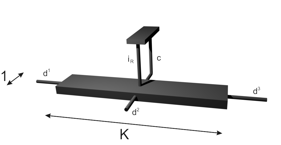
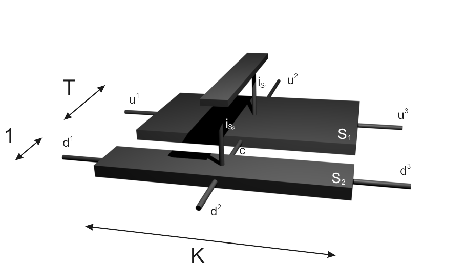
Note that the region of size 1×K1𝐾1\times K is injective when the upper and the physical system are considered as inputs (left picture of Fig. 3). To see this, take an injective region S𝑆S of dimension H×K𝐻𝐾H\times K and split it into two subregions, as in the right picture of Fig. 3 with T=H1𝑇𝐻1T=H-1. For simplicity in the rest of the proof we gather the indexes u1superscript𝑢1u^{1}, u2superscript𝑢2u^{2}, u3superscript𝑢3u^{3} and d1superscript𝑑1d^{1}, d2superscript𝑑2d^{2}, d3superscript𝑑3d^{3} and call them u𝑢u and d𝑑d respectively.

Refer to caption
Refer to caption
Figure 3: This figure represents the argument used to prove Lemma 5.

Using injectivity of the region S𝑆S, there exists {αiS1,jS2u0,d0}iS1,jS2subscriptsuperscriptsubscript𝛼subscript𝑖subscript𝑆1subscript𝑗subscript𝑆2subscript𝑢0subscript𝑑0subscript𝑖subscript𝑆1subscript𝑗subscript𝑆2\{\alpha_{i_{S_{1}},j_{S_{2}}}^{u_{0},d_{0}}\}_{i_{S_{1}},j_{S_{2}}} for any u0,d0subscript𝑢0subscript𝑑0u_{0},d_{0} such that

c,iS1,jS2αiS1,jS2u0,d0AiS1u,cAjS2c,d=δu,u0δd,d0subscript𝑐subscript𝑖subscript𝑆1subscript𝑗subscript𝑆2superscriptsubscript𝛼subscript𝑖subscript𝑆1subscript𝑗subscript𝑆2subscript𝑢0subscript𝑑0superscriptsubscript𝐴subscript𝑖subscript𝑆1𝑢𝑐superscriptsubscript𝐴subscript𝑗subscript𝑆2𝑐𝑑subscript𝛿𝑢subscript𝑢0subscript𝛿𝑑subscript𝑑0\sum_{c,i_{S_{1}},j_{S_{2}}}\alpha_{i_{S_{1}},j_{S_{2}}}^{u_{0},d_{0}}A_{i_{S_{1}}}^{u,c}A_{j_{S_{2}}}^{c,d}=\delta_{u,u_{0}}\delta_{d,d_{0}}

Taking u=u0𝑢subscript𝑢0u=u_{0} we get

c,iS1,jS2αiS1,jS2u0,d0AiS1u0,cAjS2c,d=δd,d0subscript𝑐subscript𝑖subscript𝑆1subscript𝑗subscript𝑆2superscriptsubscript𝛼subscript𝑖subscript𝑆1subscript𝑗subscript𝑆2subscript𝑢0subscript𝑑0superscriptsubscript𝐴subscript𝑖subscript𝑆1subscript𝑢0𝑐superscriptsubscript𝐴subscript𝑗subscript𝑆2𝑐𝑑subscript𝛿𝑑subscript𝑑0\sum_{c,i_{S_{1}},j_{S_{2}}}\alpha_{i_{S_{1}},j_{S_{2}}}^{u_{0},d_{0}}A_{i_{S_{1}}}^{u_{0},c}A_{j_{S_{2}}}^{c,d}=\delta_{d,d_{0}}

Now, if we take a region S𝑆S of size (H+1)×K𝐻1𝐾(H+1)\times K and divide it as in Fig. 3 with T=H𝑇𝐻T=H, there exists {βc,jS2d0}c,jS2subscriptsuperscriptsubscript𝛽𝑐subscript𝑗subscript𝑆2subscript𝑑0𝑐subscript𝑗subscript𝑆2\{\beta_{c,j_{S_{2}}}^{d_{0}}\}_{c,j_{S_{2}}} for any d0subscript𝑑0d_{0} such that

c,jS2βc,jS2d0AjS2c,d=δd,d0subscript𝑐subscript𝑗subscript𝑆2superscriptsubscript𝛽𝑐subscript𝑗subscript𝑆2subscript𝑑0superscriptsubscript𝐴subscript𝑗subscript𝑆2𝑐𝑑subscript𝛿𝑑subscript𝑑0\sum_{c,j_{S_{2}}}\beta_{c,j_{S_{2}}}^{d_{0}}A_{j_{S_{2}}}^{c,d}=\delta_{d,d_{0}}

By using injectivity of a region of dimension H×K𝐻𝐾H\times K, there exists {αiS1,jS2u0,c0,d0}iS1subscriptsuperscriptsubscript𝛼subscript𝑖subscript𝑆1subscript𝑗subscript𝑆2subscript𝑢0subscript𝑐0subscript𝑑0subscript𝑖subscript𝑆1\{\alpha_{i_{S_{1}},j_{S_{2}}}^{u_{0},c_{0},d_{0}}\}_{i_{S_{1}}} such that

iS1αiS1,jS2u0,c0,d0AiS1u,c=βc0,jS2d0δu,u0δc,c0subscriptsubscript𝑖subscript𝑆1superscriptsubscript𝛼subscript𝑖subscript𝑆1subscript𝑗subscript𝑆2subscript𝑢0subscript𝑐0subscript𝑑0superscriptsubscript𝐴subscript𝑖subscript𝑆1𝑢𝑐superscriptsubscript𝛽subscript𝑐0subscript𝑗subscript𝑆2subscript𝑑0subscript𝛿𝑢subscript𝑢0subscript𝛿𝑐subscript𝑐0\sum_{i_{S_{1}}}\alpha_{i_{S_{1}},j_{S_{2}}}^{u_{0},c_{0},d_{0}}A_{i_{S_{1}}}^{u,c}=\beta_{c_{0},j_{S_{2}}}^{d_{0}}\delta_{u,u_{0}}\delta_{c,c_{0}}

By putting both equalities together, we find

c,c0,iS1,jS2αiS1,jS2u0,c0,d0AiS1u,cAjS2c,d=subscript𝑐subscript𝑐0subscript𝑖subscript𝑆1subscript𝑗subscript𝑆2superscriptsubscript𝛼subscript𝑖subscript𝑆1subscript𝑗subscript𝑆2subscript𝑢0subscript𝑐0subscript𝑑0superscriptsubscript𝐴subscript𝑖subscript𝑆1𝑢𝑐superscriptsubscript𝐴subscript𝑗subscript𝑆2𝑐𝑑absent\displaystyle\sum_{c,c_{0},i_{S_{1}},j_{S_{2}}}\alpha_{i_{S_{1}},j_{S_{2}}}^{u_{0},c_{0},d_{0}}A_{i_{S_{1}}}^{u,c}A_{j_{S_{2}}}^{c,d}=
=c,c0jS2βc0,jS2d0δu,u0δc,c0AjS2c,d=absentsubscript𝑐subscript𝑐0subscript𝑗subscript𝑆2superscriptsubscript𝛽subscript𝑐0subscript𝑗subscript𝑆2subscript𝑑0subscript𝛿𝑢subscript𝑢0subscript𝛿𝑐subscript𝑐0superscriptsubscript𝐴subscript𝑗subscript𝑆2𝑐𝑑absent\displaystyle=\sum_{c,c_{0}j_{S_{2}}}\beta_{c_{0},j_{S_{2}}}^{d_{0}}\delta_{u,u_{0}}\delta_{c,c_{0}}A_{j_{S_{2}}}^{c,d}=
=c0jS2βc0,jS2d0δu,u0AjS2c0,d=δu,u0δd,d0absentsubscriptsubscript𝑐0subscript𝑗subscript𝑆2superscriptsubscript𝛽subscript𝑐0subscript𝑗subscript𝑆2subscript𝑑0subscript𝛿𝑢subscript𝑢0superscriptsubscript𝐴subscript𝑗subscript𝑆2subscript𝑐0𝑑subscript𝛿𝑢subscript𝑢0subscript𝛿𝑑subscript𝑑0\displaystyle=\sum_{c_{0}j_{S_{2}}}\beta_{c_{0},j_{S_{2}}}^{d_{0}}\delta_{u,u_{0}}A_{j_{S_{2}}}^{c_{0},d}=\delta_{u,u_{0}}\delta_{d,d_{0}}

and so S𝑆S is an injective region. ∎

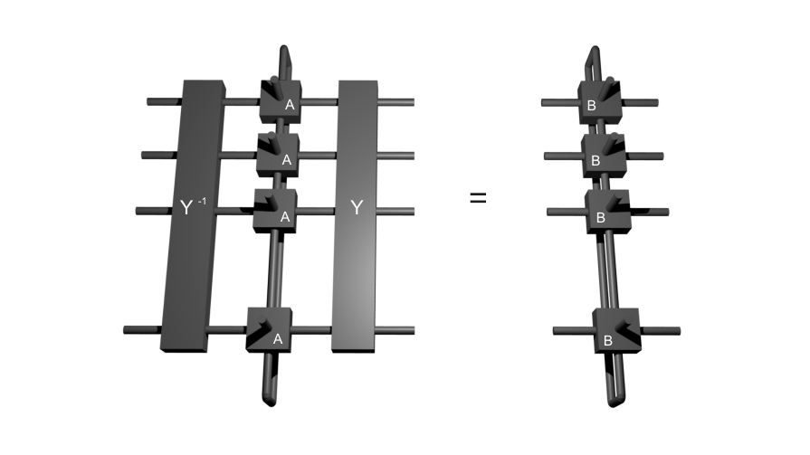
This allows us to reduce the 2D case to the 1D case by grouping all the tensors in a column. The 1D case (Theorem 2) ensures that there is a global invertible matrix Y𝑌Y which verifies the equality in Fig. 4. Now
Refer to caption
Figure 4: Translational invariance and injectivity allow to reduce the 2D case to the 1D case.
Lemma 6.

Y𝑌Y maps product vectors into product vectors.

We will show that Y𝑌Y maps any product vector to a vector with the property:

(*) It is a product in any bipartition R-S, for regions R and S of consecutive spins and size L/5absent𝐿5\geq L/5.

Since any vector with property (*) is trivially a product vector, this would finish the proof. So let us take a product i|xisubscripttensor-product𝑖absentketsubscript𝑥𝑖\otimes_{i}|x_{i}\rangle and assume that this product is mapped by Y𝑌Y into a vector that can be written in some orthonormal bases as Y(i|xi)=r=1,2,βr|vrwrY(\otimes_{i}|x_{i}\rangle)=\sum_{r=1,2,\ldots}\beta_{r}|v_{r}w_{r}\rangle in a partition R-S for regions of consecutive spins and size L/5absent𝐿5\geq L/5. For the same bipartition, we may write ixi|Y1=r=1,2,αrvrwr|\otimes_{i}\langle x_{i}|Y^{-1}=\sum_{r=1,2,\ldots}\alpha_{r}\langle v^{\prime}_{r}w^{\prime}_{r}|, which could be a product. We group N/5𝑁5N/5 columns, sandwich with i|xisubscripttensor-product𝑖absentketsubscript𝑥𝑖\otimes_{i}|x_{i}\rangle in Fig 4 and analyze the Schmidt rank between the two physical R×N/5𝑅𝑁5R\times N/5 and S×N/5𝑆𝑁5S\times N/5 systems in both the right and left part of Fig. 4. It clearly gives D2N/5superscript𝐷2𝑁5D^{2N/5} in the RHS by using injectivity. By performing the changes of bases |r|vrmaps-toket𝑟ketsubscript𝑣𝑟|r\rangle\mapsto|v_{r}\rangle and |r|wrmaps-toket𝑟ketsubscript𝑤𝑟|r\rangle\mapsto|w_{r}\rangle (and the same for the primes) to the tensors AR×N/5superscript𝐴𝑅𝑁5A^{R\times N/5} and AS×N/5superscript𝐴𝑆𝑁5A^{S\times N/5} in the LHS, it gives new tensors Asuperscript𝐴A^{\prime} and A′′superscript𝐴′′A^{\prime\prime} for which we get

abcdαaβc[iAabcdi|i][jAadcb′′j|j]subscript𝑎𝑏𝑐𝑑subscript𝛼𝑎subscript𝛽𝑐delimited-[]subscript𝑖subscriptsuperscript𝐴𝑖𝑎𝑏𝑐𝑑ket𝑖delimited-[]subscript𝑗subscriptsuperscript𝐴′′𝑗𝑎𝑑𝑐𝑏ket𝑗\sum_{abcd}\alpha_{a}{\beta}_{c}[\sum_{i}A^{\prime i}_{abcd}|i\rangle][\sum_{j}A^{\prime\prime j}_{adcb}|j\rangle]

By means of injectivity, we know that the set {iAabcdi|i}abcdsubscriptsubscript𝑖subscriptsuperscript𝐴𝑖𝑎𝑏𝑐𝑑ket𝑖𝑎𝑏𝑐𝑑\{\sum_{i}A^{\prime i}_{abcd}|i\rangle\}_{abcd} is linearly independent (and the same for A′′superscript𝐴′′A^{\prime\prime}). This means that the Schmidt rank of the LHS is at least 2D2N/52superscript𝐷2𝑁52D^{2N/5}, which is the desired contradiction.

The following three lemmas specify the form of Y𝑌Y:

Lemma 7.

If Y𝑌Y is invertible and takes products to products it is of the form Pπ(Y1YL)subscript𝑃𝜋tensor-productsubscript𝑌1subscript𝑌𝐿P_{\pi}(Y_{1}\otimes\cdots\otimes Y_{L}) where Pπsubscript𝑃𝜋P_{\pi} implements a permutation π𝜋\pi of the Hilbert spaces.

Proof.

We reason for simplicity in the bipartite case—the argument generalizes straightforwardly to the general case by induction. Let Y:dddd:𝑌tensor-productsuperscript𝑑superscript𝑑tensor-productsuperscript𝑑superscript𝑑Y:\mathbbm{C}^{d}\otimes\mathbbm{C}^{d}\longrightarrow\mathbbm{C}^{d}\otimes\mathbbm{C}^{d} be invertible which takes products to products and denote {|i,j}i,j=1,,dsubscriptket𝑖𝑗formulae-sequence𝑖𝑗1𝑑\{|i,j\rangle\}_{i,j=1,...,d} the product basis. Let Y(|i,1)=|αi,βi𝑌ket𝑖1ketsubscript𝛼𝑖subscript𝛽𝑖Y(|i,1\rangle)=|\alpha_{i},\beta_{i}\rangle. Take i0i1{1,,d}subscript𝑖0subscript𝑖11𝑑i_{0}\neq i_{1}\in\{1,...,d\}, then Y(|i0,1+|i1,1)=|αi0,βi0+|αi1,βi1𝑌ketsubscript𝑖01ketsubscript𝑖11ketsubscript𝛼subscript𝑖0subscript𝛽subscript𝑖0ketsubscript𝛼subscript𝑖1subscript𝛽subscript𝑖1Y(|i_{0},1\rangle+|i_{1},1\rangle)=|\alpha_{i_{0}},\beta_{i_{0}}\rangle+|\alpha_{i_{1}},\beta_{i_{1}}\rangle is a product and, as Y𝑌Y is invertible, then either I) αi0αi1proportional-tosubscript𝛼subscript𝑖0subscript𝛼subscript𝑖1\alpha_{i_{0}}\propto\alpha_{i_{1}} & βi0∝̸βi1not-proportional-tosubscript𝛽subscript𝑖0subscript𝛽subscript𝑖1\beta_{i_{0}}\not\propto\beta_{i_{1}} or II) αi0∝̸αi1not-proportional-tosubscript𝛼subscript𝑖0subscript𝛼subscript𝑖1\alpha_{i_{0}}\not\propto\alpha_{i_{1}} & βi0βi1proportional-tosubscript𝛽subscript𝑖0subscript𝛽subscript𝑖1\beta_{i_{0}}\propto\beta_{i_{1}}, where proportional-to\propto means proportional to. In fact, we are always in the same case: if d=2𝑑2d=2 there is only one case, otherwise take three distinct i0,i1,i2{1,,d}subscript𝑖0subscript𝑖1subscript𝑖21𝑑i_{0},i_{1},i_{2}\in\{1,...,d\} such that αi0∝̸αi1not-proportional-tosubscript𝛼subscript𝑖0subscript𝛼subscript𝑖1\alpha_{i_{0}}\not\propto\alpha_{i_{1}} and βi1∝̸βi2not-proportional-tosubscript𝛽subscript𝑖1subscript𝛽subscript𝑖2\beta_{i_{1}}\not\propto\beta_{i_{2}} then we get a contradiction from the fact that Y(|i0,1+|i2,1)𝑌ketsubscript𝑖01ketsubscript𝑖21Y(|i_{0},1\rangle+|i_{2},1\rangle) is a product.

The same argumentation can be carried out for the second tensor. We can therefore assume w.l.o.g. that

Y(|i,1)=|αi,β1𝑌ket𝑖1ketsubscript𝛼𝑖subscript𝛽1Y(|i,1\rangle)=|\alpha_{i},\beta_{1}\rangle

and

Y(|1,j)=|α1,βj𝑌ket1𝑗ketsubscript𝛼1subscript𝛽𝑗Y(|1,j\rangle)=|\alpha_{1},\beta_{j}\rangle

In the other case, we just permute the indexes by means of the swap operator Pπsubscript𝑃𝜋P_{\pi}.

Let us consider Y(|i,j)=|ai,j,bi,j𝑌ket𝑖𝑗ketsubscript𝑎𝑖𝑗subscript𝑏𝑖𝑗Y(|i,j\rangle)=|a_{i,j},b_{i,j}\rangle. Now, since

Y(|i,j+|i,1)=|αi,β1+|ai,j,bi,j𝑌ket𝑖𝑗ket𝑖1ketsubscript𝛼𝑖subscript𝛽1ketsubscript𝑎𝑖𝑗subscript𝑏𝑖𝑗Y(|i,j\rangle+|i,1\rangle)=|\alpha_{i},\beta_{1}\rangle+|a_{i,j},b_{i,j}\rangle

is a product, we obtain that αiai,jproportional-tosubscript𝛼𝑖subscript𝑎𝑖𝑗\alpha_{i}\propto a_{i,j} or β1bi,jproportional-tosubscript𝛽1subscript𝑏𝑖𝑗\beta_{1}\propto b_{i,j}. However, the second case is only possible if j=1𝑗1j=1 because of the invertibility of Y𝑌Y, and then ai,jαiproportional-tosubscript𝑎𝑖𝑗subscript𝛼𝑖a_{i,j}\propto\alpha_{i}. A similar argumentation over the second tensor gives Y(|i,j)=ci,j|αi,βj𝑌ket𝑖𝑗subscript𝑐𝑖𝑗ketsubscript𝛼𝑖subscript𝛽𝑗Y(|i,j\rangle)=c_{i,j}|\alpha_{i},\beta_{j}\rangle. Now making Y(i,j=1d|ij)=i,j=1dci,j|αi,βj𝑌superscriptsubscript𝑖𝑗1𝑑ket𝑖𝑗superscriptsubscript𝑖𝑗1𝑑subscript𝑐𝑖𝑗ketsubscript𝛼𝑖subscript𝛽𝑗Y(\sum_{i,j=1}^{d}|ij\rangle)=\sum_{i,j=1}^{d}c_{i,j}|\alpha_{i},\beta_{j}\rangle and knowing that the Schmidt rank of the resulting vector must be one, we conclude that the matrix (ci,j)i,jsubscriptsubscript𝑐𝑖𝑗𝑖𝑗(c_{i,j})_{i,j} has rank one and therefore is of the form ci,j=risjsubscript𝑐𝑖𝑗subscript𝑟𝑖subscript𝑠𝑗c_{i,j}=r_{i}s_{j} giving Y(|i,j)=|riαi,sjβj𝑌ket𝑖𝑗ketsubscript𝑟𝑖subscript𝛼𝑖subscript𝑠𝑗subscript𝛽𝑗Y(|i,j\rangle)=|r_{i}\alpha_{i},s_{j}\beta_{j}\rangle, the desired result. ∎

Let us now show that Pπsubscript𝑃𝜋P_{\pi} is the trivial permutation:

Lemma 8.

Pπ=𝟙subscript𝑃𝜋1P_{\pi}=\mathbbm{1}

Proof.

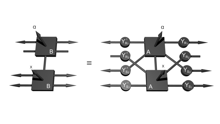
Assume that Pπsubscript𝑃𝜋P_{\pi} is not the identity. Take a RS𝑅𝑆R-S bipartition (with sizes L/5absent𝐿5\geq L/5) such that Pπsubscript𝑃𝜋P_{\pi} maps one Hilbert space of R𝑅R into one of S𝑆S. We block again N/5𝑁5N/5 columns to get two injective R×N/5𝑅𝑁5R\times N/5 and S×N/5𝑆𝑁5S\times N/5 regions. Denoting by R1subscript𝑅1R_{1} and S1subscript𝑆1S_{1} the parts of the regions that stay within the regions and by R2subscript𝑅2R_{2}, S2subscript𝑆2S_{2} the ones that are mapped to the other side, we can decompose Y𝑌Y as in Fig. 5.

Refer to caption
Figure 5: The cones represent vectors multiplying the legs of the tensor. In the virtual space, these vectors are |0ket0|0\rangle, while the vectors in the leg corresponding to the real space are |xket𝑥|x\rangle and |αket𝛼|\alpha\rangle respectively.

Consider now Fig.5. We contract all virtual indices but the pair in the second row with |0ket0|0\rangle and the physical indices with |αket𝛼|\alpha\rangle and |xket𝑥|x\rangle where the latter is chosen such that A|x=|0|0|0|0𝐴ket𝑥ket0ket0ket0ket0A|x\rangle=|0\rangle|0\rangle|0\rangle|0\rangle. Let V𝑉V be the span in the remaining two virtual indices under the variation of |αket𝛼|\alpha\rangle. It is clear that in the LHS of Fig.5, dimV=dim(support(YR2))dimension𝑉dimensionsupportsubscript𝑌subscript𝑅2\dim V=\dim{({\rm support}{(Y_{R_{2}})})}, whereas in the RHS dimV=1dimension𝑉1\dim V=1, which leads to a contradiction unless R2subscript𝑅2R_{2} and S2subscript𝑆2S_{2} are empty. ∎

By using both, injectivity and translational invariance of the RHS in Fig. 4, we observe that

Lemma 9.

Yi=Ysubscript𝑌𝑖𝑌Y_{i}=Y for all i𝑖i.

We redefine now Aisuperscript𝐴𝑖A^{i} as ldruAldrui(Y1𝟙)|ldru|(Y𝟙)subscript𝑙𝑑𝑟𝑢subscriptsuperscript𝐴𝑖𝑙𝑑𝑟𝑢tensor-productsuperscript𝑌11ket𝑙𝑑bra𝑟𝑢tensor-product𝑌1\sum_{ldru}A^{i}_{ldru}(Y^{-1}\otimes\mathbbm{1})|ld\rangle\langle ru|(Y\otimes\mathbbm{1}), block N/5𝑁5N/5 columns together and sandwich with |nnnket𝑛𝑛𝑛|nn\cdots n\rangle and mmm|bra𝑚𝑚𝑚\langle mm\cdots m| in Fig. 4. Defining A~i;mnsuperscript~𝐴𝑖𝑚𝑛\tilde{A}^{i;mn} as

bdA~bdi;mn|bd|=bdm|A1×N/5|n|bd|subscript𝑏𝑑subscriptsuperscript~𝐴𝑖𝑚𝑛𝑏𝑑ket𝑏bra𝑑subscript𝑏𝑑quantum-operator-product𝑚superscript𝐴1𝑁5𝑛ket𝑏bra𝑑\sum_{bd}\tilde{A}^{i;mn}_{bd}|b\rangle\langle d|=\sum_{bd}\langle m|A^{1\times N/5}|n\rangle|b\rangle\langle d|

and the analog for B~i;mnsuperscript~𝐵𝑖𝑚𝑛\tilde{B}^{i;mn}, we have two injective representations of the same MPS. By means of the 1D case (Theorem 2), we obtain invertible matrices Znmsubscript𝑍𝑛𝑚Z_{nm} such that Zmn1A~i;mnZmn=B~i;mnsubscriptsuperscript𝑍1𝑚𝑛superscript~𝐴𝑖𝑚𝑛subscript𝑍𝑚𝑛superscript~𝐵𝑖𝑚𝑛Z^{-1}_{mn}\tilde{A}^{i;mn}Z_{mn}=\tilde{B}^{i;mn}.

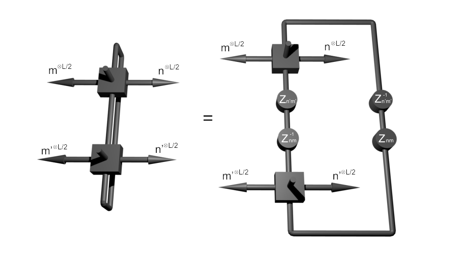
The next step is to show that Zmnsubscript𝑍𝑚𝑛Z_{mn} does not depend on m𝑚m and n𝑛n. We sandwich in Fig. 4 with m|L/2m|L/2superscriptbrasuperscript𝑚tensor-productabsent𝐿2superscriptbra𝑚tensor-productabsent𝐿2\langle{m^{\prime}}|^{\otimes L/2}\langle m|^{\otimes L/2} and |nL/2|nL/2superscriptketsuperscript𝑛tensor-productabsent𝐿2superscriptket𝑛tensor-productabsent𝐿2|{n^{\prime}}\rangle^{\otimes L/2}|n\rangle^{\otimes L/2} and get Fig. 6. By summing with appropriate coefficients in order to obtain ”deltas”, we obtain that l|ZmnZmn1|kr|Zmn1Zmn|s=δklδrsquantum-operator-product𝑙subscript𝑍𝑚𝑛subscriptsuperscript𝑍1superscript𝑚superscript𝑛𝑘quantum-operator-product𝑟superscriptsubscript𝑍𝑚𝑛1subscript𝑍superscript𝑚superscript𝑛𝑠subscript𝛿𝑘𝑙subscript𝛿𝑟𝑠\langle l|Z_{mn}Z^{-1}_{m^{\prime}n^{\prime}}|k\rangle\langle r|Z_{mn}^{-1}Z_{m^{\prime}n^{\prime}}|s\rangle=\delta_{kl}\delta_{rs}, so Zmn=Zsuperscript𝑍𝑚𝑛𝑍Z^{mn}=Z is indeed independent of m𝑚m and n𝑛n. By reasoning as above in the other direction, one can prove that Z=ZN/5𝑍superscript𝑍tensor-productabsent𝑁5Z=Z^{\prime\otimes N/5}.

Refer to caption
Figure 6: This is a representation of the resulting tensor after blocking L2×N5𝐿2𝑁5\frac{L}{2}\times\frac{N}{5} sites. The vectors in the virtual space correspond to tensor products of L2𝐿2\frac{L}{2} local vectors.

Up to now, we have proven the following Lemma

Lemma 10.

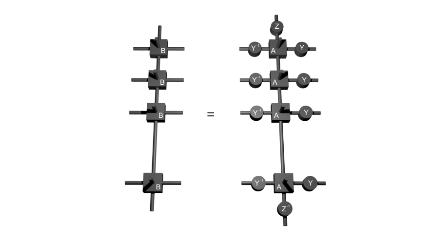
For any length H𝐻H for which one gets injectivity in the orthogonal direction, we have the structure shown in Fig. 7. The case where vertical is interchanged by horizontal is equivalent.
Refer to caption
Figure 7: A subsystem of H𝐻H spins has two equivalent injective TI-PEPS representations iff they are connected by invertible matrices.

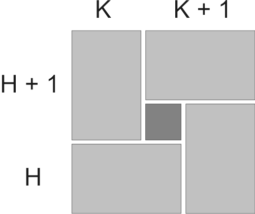
We want to prove now Theorem 4. Let us consider a H×K𝐻𝐾H\times K injective region, for instance H=L/5𝐻𝐿5H=L/5, K=N/5𝐾𝑁5K=N/5. From Lemma 5, the larger regions in Fig. 8 are also injective. If we replace Fig. 7 first in each subregion (not the center), and then in the whole region, we get the desired result by using injectivity in the four subregions.
Refer to caption
Figure 8: Representation of the regions of injectivity for the proof of Theorem 4.

As we said in the introduction of this section, we can generalize Theorem 4 to the honeycomb lattice. We need to prove first the following

Lemma 11.

Let A,Cd1,d2𝐴𝐶subscriptsubscript𝑑1subscript𝑑2A,C\in\mathcal{M}_{d_{1},d_{2}} and B,Dd2,d3𝐵𝐷subscriptsubscript𝑑2subscript𝑑3B,D\in\mathcal{M}_{d_{2},d_{3}} and let us assume that min(d1,d2,d3)=d2subscript𝑑1subscript𝑑2subscript𝑑3subscript𝑑2\min(d_{1},d_{2},d_{3})=d_{2}. Then, if AB=CD𝐴𝐵𝐶𝐷AB=CD and rank(B)=rank(D)=d2rank𝐵rank𝐷subscript𝑑2\operatorname{rank}(B)=\operatorname{rank}(D)=d_{2} there exists an invertible matrix W𝑊W such that A=CW𝐴𝐶𝑊A=CW and B=W1D𝐵superscript𝑊1𝐷B=W^{-1}D.

Proof.

Since B𝐵B is full-rank and min(d1,d2,d3)=d2subscript𝑑1subscript𝑑2subscript𝑑3subscript𝑑2\min(d_{1},d_{2},d_{3})=d_{2}, there exists a matrix that we can call B1superscript𝐵1B^{-1} such that BB1=𝟙d2𝐵superscript𝐵1subscript1subscript𝑑2BB^{-1}=\mathbbm{1}_{d_{2}}. Therefore, A=C(DB1)𝐴𝐶𝐷superscript𝐵1A=C(DB^{-1}) and we can denote W=DB1𝑊𝐷superscript𝐵1W=DB^{-1}, which is an invertible matrix. Similarly B=A1CD𝐵superscript𝐴1𝐶𝐷B=A^{-1}CD and we can denote U=A1C𝑈superscript𝐴1𝐶U=A^{-1}C. Since UW=A1CDB1=BB1=𝟙d2𝑈𝑊superscript𝐴1𝐶𝐷superscript𝐵1𝐵superscript𝐵1subscript1subscript𝑑2UW=A^{-1}CDB^{-1}=BB^{-1}=\mathbbm{1}_{d_{2}}, we get that U=W1𝑈superscript𝑊1U=W^{-1} and hence B=W1D𝐵superscript𝑊1𝐷B=W^{-1}D. ∎

We can now prove the theorem for the honeycomb lattice. Let us remark that the unit cell of this lattice contains two sites and that the lattice associated to the unit cells is a square lattice. The translational invariance is not site by site, but unit cell by unit cell.

Theorem 12 (The honeycomb lattice).
Let |ΨketΨ|\Psi\rangle and |ΨketsuperscriptΨ|\Psi^{\prime}\rangle be two PEPS defined in a honeycomb lattice and such that the square lattice constituted by the unit cells fulfils the conditions of Theorem 4. Then, |Ψ=|ΨketΨketsuperscriptΨ|\Psi\rangle=|\Psi^{\prime}\rangle iff the conditions shown in Fig. 9 hold.

Refer to caption
Figure 9: These are the relations which the tensors defining two TI-PEPS on a honeycomb lattice must fulfil in order to represent the same state.
Proof.

Let us apply Theorem 4 to the square lattice which the unit cell constitutes. Then, we obtain the equality shown in Fig. 10 and Lemma 11 completes the proof of the theorem. ∎

Refer to caption
Figure 10: The possibility of transforming the honeycomb lattice into a square lattice by blocking tensors enables us to apply the result on equivalent TI-PEPS representations for the square lattice.

IV Symmetries

String order parameters have been proven to be a very useful tool in the detection and understanding of quantum phase transitions. However, as pointed out in Anfuso its application could not go beyond the 1D case. In PWSVC08 , with the aid of MPS, it has been shown that the existence of a string order parameter is intimately related to the existence of a symmetry, which allows to design an appropriate 2D definition: the existence of a local symmetry when we consider increasing sizes of the system. A trivial sufficient condition for this to hold in PEPS is proposed there (see Fig. 11), and further analyzed in Vidal-symm in the more general context of Tensor Network States. The aim of this section is to prove that, for injective PEPS, the condition is also necessary. The 1D version is proven in PWSVC08 with the assumption of injectivity and in SWPC09 for the general 1D case.

Theorem 13 (Local symmetry).

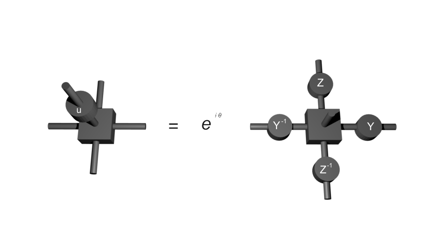
If a TI-PEPS defined on an L×N𝐿𝑁L\times N lattice has a symmetry u𝑢u, i.e. uNL|ψA=eiθ|ψAsuperscript𝑢tensor-productabsent𝑁𝐿ketsubscript𝜓𝐴superscript𝑒𝑖superscript𝜃ketsubscript𝜓𝐴u^{\otimes NL}|\psi_{A}\rangle=e^{i\theta^{\prime}}|\psi_{A}\rangle, and is injective in regions of size L/5×N/5𝐿5𝑁5L/5\times N/5, then the tensors defining it satisfy the relation in Fig. 11 with eiθNL=eiθsuperscript𝑒𝑖𝜃𝑁𝐿superscript𝑒𝑖superscript𝜃e^{i\theta NL}=e^{i\theta^{\prime}}. Moreover, if ugsubscript𝑢𝑔u_{g} is a representation of a continuous group G𝐺G, then Ygsubscript𝑌𝑔Y_{g}, Zgsubscript𝑍𝑔Z_{g} and eiθgsuperscript𝑒𝑖subscript𝜃𝑔e^{i\theta_{g}} are representations as well.

Refer to caption
Figure 11: This is a graphical representation of the equation that a PEPS fulfils if it is invariant under a representation ugsubscript𝑢𝑔u_{g} of a group G𝐺G. Then, the symmetry is inherited into a couple of representations of G𝐺G, called Ygsubscript𝑌𝑔Y_{g} and Zgsubscript𝑍𝑔Z_{g}, up to a phase eiθgsuperscript𝑒𝑖subscript𝜃𝑔e^{i\theta_{g}}.
Proof.

Notice that when acting with u𝑢u and eiθsuperscript𝑒𝑖𝜃e^{-i\theta} on the tensor A𝐴A which defines the PEPS (see Fig 11), we get a new tensor B𝐵B that is also injective in regions of size L/5×N/5𝐿5𝑁5L/5\times N/5 and such that |ψA=|ψBketsubscript𝜓𝐴ketsubscript𝜓𝐵|\psi_{A}\rangle=|\psi_{B}\rangle. Theorem 4 then gives the result. In order to prove that the invertible matrices Ygsubscript𝑌𝑔Y_{g} and Zgsubscript𝑍𝑔Z_{g} are representations of G𝐺G, we only need to follow the arguments used in (SWPC09, , Theorem 7). ∎

With exactly the same reasoning, we can characterize the spatial symmetries: reflection, π/2𝜋2\pi/2-rotations and π𝜋\pi-rotations:

Theorem 14 (Reflection symmetry).

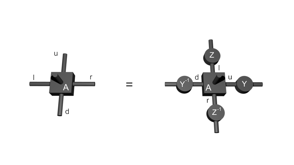
Let us consider an L×N𝐿𝑁L\times N TI-PEPS with the property that for a region of size smaller than L/5×N/5𝐿5𝑁5L/5\times N/5 it is injective. If this PEPS is invariant under a reflection with respect to a vertical axis, then there exist invertible matrices Y𝑌Y, Z𝑍Z such that the tensors defining the PEPS verify Fig. 12, that is, ldruAldruildru|=(ldruAldruirdlu|)YZY1Z1subscript𝑙𝑑𝑟𝑢subscriptsuperscript𝐴𝑖𝑙𝑑𝑟𝑢bra𝑙𝑑𝑟𝑢tensor-productsubscript𝑙𝑑𝑟𝑢subscriptsuperscript𝐴𝑖𝑙𝑑𝑟𝑢bra𝑟𝑑𝑙𝑢𝑌𝑍superscript𝑌1superscript𝑍1\sum_{ldru}A^{i}_{ldru}\langle ldru|=(\sum_{ldru}A^{i}_{ldru}\langle rdlu|)Y\otimes Z\otimes Y^{-1}\otimes Z^{-1} for all i𝑖i.

Refer to caption
Figure 12: This figure represents the condition which must be fulfilled by a TI-PEPS in order to generate a state invariant under reflections (in this case with respect to the horizontal plane).

Moreover, it is easy to see that Y,Z𝑌𝑍Y,Z must satisfy YT=Ysuperscript𝑌𝑇𝑌Y^{T}=Y, Z2=𝟙superscript𝑍21Z^{2}=\mathbbm{1}. The characterization of the reflection with respect to the horizontal axis follows straightforwardly by changing the roles of the horizontal/vertical directions.

Theorem 15 (spatial π/2𝜋2\pi/2-rotation symmetry).

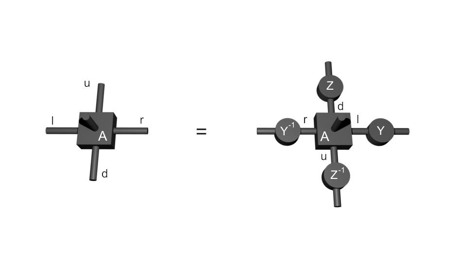
If an L×N𝐿𝑁L\times N TI-PEPS with the property that for a region of size smaller than L/5×N/5𝐿5𝑁5L/5\times N/5 it is injective has a spatial π/2𝜋2\pi/2-rotation invariance, then there exist invertible matrices Y𝑌Y, Z𝑍Z such that the tensors Aisuperscript𝐴𝑖A^{i} defining the PEPS verify Fig. 13, that is, ldruAldruildru|=(ldruAldruiuldr|)YZY1Z1subscript𝑙𝑑𝑟𝑢subscriptsuperscript𝐴𝑖𝑙𝑑𝑟𝑢bra𝑙𝑑𝑟𝑢tensor-productsubscript𝑙𝑑𝑟𝑢subscriptsuperscript𝐴𝑖𝑙𝑑𝑟𝑢bra𝑢𝑙𝑑𝑟𝑌𝑍superscript𝑌1superscript𝑍1\sum_{ldru}A^{i}_{ldru}\langle ldru|=(\sum_{ldru}A^{i}_{ldru}\langle uldr|)Y\otimes Z\otimes Y^{-1}\otimes Z^{-1} for all i𝑖i.

Refer to caption
Figure 13: This figure represents the condition which must be fulfilled by a TI-PEPS in order to generate a state invariant under π2𝜋2\frac{\pi}{2}-rotations (in this case a clockwise rotation).

In this case, one can see that Y𝑌Y, Z𝑍Z must satisfy the additional constraints (YZ)T=YZsuperscript𝑌𝑍𝑇𝑌𝑍(YZ)^{T}=YZ, (ZY)T=ZYsuperscript𝑍𝑌𝑇𝑍𝑌(ZY)^{T}=ZY.

Finally, we characterize the PEPS which are symmetric respect to a π𝜋\pi-rotation.

Theorem 16 (spatial π𝜋\pi-rotation symmetry).

Let us consider an L×N𝐿𝑁L\times N TI-PEPS with the property that for a region of size smaller than L/5×N/5𝐿5𝑁5L/5\times N/5 it is injective and that it is invariant under a π𝜋\pi-rotation, then there exist invertible matrices Y𝑌Y, Z𝑍Z such that the tensors defining the PEPS verify Fig. 14, that is, ldruAldruildru|=(ldruAldruiruld|)YZY1Z1subscript𝑙𝑑𝑟𝑢subscriptsuperscript𝐴𝑖𝑙𝑑𝑟𝑢bra𝑙𝑑𝑟𝑢tensor-productsubscript𝑙𝑑𝑟𝑢subscriptsuperscript𝐴𝑖𝑙𝑑𝑟𝑢bra𝑟𝑢𝑙𝑑𝑌𝑍superscript𝑌1superscript𝑍1\sum_{ldru}A^{i}_{ldru}\langle ldru|=(\sum_{ldru}A^{i}_{ldru}\langle ruld|)Y\otimes Z\otimes Y^{-1}\otimes Z^{-1} for all i𝑖i.

Now the constraints are ZT=Zsuperscript𝑍𝑇𝑍Z^{T}=Z, YT=Ysuperscript𝑌𝑇𝑌Y^{T}=Y.

Refer to caption
Figure 14: This figure represents the condition which must be fulfilled by a TI-PEPS in order to generate a state invariant under π𝜋\pi-rotations (in this case a clockwise rotation).

V Applications

It is clear that a symmetry must imposes restrictions on the possible behaviors and properties of a quantum system. Understanding these restrictions is a hard problem that has led the research in Quantum Many Body Physics in the last decades. For PEPS, which seem to provide a reasonably complete description of quantum states, we have proven a simple characterization of the existence of symmetries, which immediately leads to a number of consequences. In the lines below we list some of them.

V.1 Lieb-Schultz-Mattis Theorem

The Lieb-Schultz-Mattis theorem states that, for semi-integer spin, a SU(2)𝑆𝑈2SU(2)-invariant 1D Hamiltonian cannot have a uniform (independent of the size of the system) energy gap. This theorem has been generalized in a number of ways. Still in the 1D case but relaxing the symmetry to a U(1)𝑈1U(1) symmetry, Oshikawa, Yamanaka and Affleck showed in OYA97 that the same conclusion holds if Jm𝐽𝑚J-m is not an integer, where J𝐽J is the spin and m𝑚m the magnetization per particle. For the SU(2)𝑆𝑈2SU(2) case in 2D, Hastings and Nachtergaele-Sims proved that the same results holds HastingsLSM . In SWPC09 , we showed how the orginial Lieb-Schultz-Mattis Theorem can be understood on the level of states. More precisely, we showed that any SU(2)𝑆𝑈2SU(2) invariant MPS with semi-integer spin cannot be injective. In this section we will give a 2D version of the Oshikawa-Yamanaka-Affleck theorem, by showing that a U(1)𝑈1U(1) symmetric PEPS for which Jm𝐽𝑚J-m is not an integer cannot be injective.

Let us start with a PEPS |ψAketsubscript𝜓𝐴|\psi_{A}\rangle of spin J𝐽J particles with a U(1)𝑈1U(1) symmetry in the z𝑧z direction, that is

ugN|ψA=eiθg|ψAsuperscriptsubscript𝑢𝑔tensor-productabsent𝑁ketsubscript𝜓𝐴superscript𝑒𝑖subscript𝜃𝑔ketsubscript𝜓𝐴u_{g}^{\otimes N}|\psi_{A}\rangle=e^{i\theta_{g}}|\psi_{A}\rangle

with ug=eigSzsubscript𝑢𝑔superscript𝑒𝑖𝑔subscript𝑆𝑧u_{g}=e^{igS_{z}}. Since geiθgmaps-to𝑔superscript𝑒𝑖subscript𝜃𝑔g\mapsto e^{i\theta_{g}} is clearly a representation, there exists θ𝜃\theta such that θg=Ngθsubscript𝜃𝑔𝑁𝑔𝜃\theta_{g}=Ng\theta. We will show that

Lemma 17.

θ𝜃\theta coincides with the magnetization per particle m𝑚m.

To see this it is enough to expand both sides of the expression ugN|ψA=eiNgθ|ψAsuperscriptsubscript𝑢𝑔tensor-productabsent𝑁ketsubscript𝜓𝐴superscript𝑒𝑖𝑁𝑔𝜃ketsubscript𝜓𝐴u_{g}^{\otimes N}|\psi_{A}\rangle=e^{iNg\theta}|\psi_{A}\rangle around the identity: from the LHS we get ugN|ψA(𝟙+igjSjz)|ψAsimilar-to-or-equalssuperscriptsubscript𝑢𝑔tensor-productabsent𝑁ketsubscript𝜓𝐴1𝑖𝑔subscript𝑗superscriptsubscript𝑆𝑗𝑧ketsubscript𝜓𝐴u_{g}^{\otimes N}|\psi_{A}\rangle\simeq(\mathbbm{1}+ig\sum_{j}S_{j}^{z})|\psi_{A}\rangle, while the RHS gives (1+iNgθ)|ψA1𝑖𝑁𝑔𝜃ketsubscript𝜓𝐴(1+iN\vec{g}\cdot\vec{\theta})|\psi_{A}\rangle. By simplifying both results, we get θ=ψA|jSjz|ψA𝜃quantum-operator-productsubscript𝜓𝐴subscript𝑗superscriptsubscript𝑆𝑗𝑧subscript𝜓𝐴\theta=\langle\psi_{A}|\sum_{j}S_{j}^{z}|\psi_{A}\rangle, the desired result.

Now we can prove the announced generalized Lieb-Schulz-Mattis theorem for PEPS.

Theorem 18.

Let us consider a PEPS |ψAketsubscript𝜓𝐴|\psi_{A}\rangle in a square L×N𝐿𝑁L\times N lattice that is injective in regions of size L/5×N/5𝐿5𝑁5L/5\times N/5. If |ψAketsubscript𝜓𝐴|\psi_{A}\rangle is invariant under a representation of U(1)𝑈1U(1) with the usual generator of spin J𝐽J given by Sz(J)subscriptsuperscript𝑆𝐽𝑧S^{(J)}_{z}, then the magnetization per particle m𝑚m fulfils that (Jm)𝐽𝑚(J-m) is an integer.

If the state has full SU(2)𝑆𝑈2SU(2) symmetry, then m=0𝑚0m=0 and we get the “Lieb-Schultz-Mattis theorem” for PEPS.

Proof.

We will choose RL/5𝑅𝐿5R\geq L/5, SN/5𝑆𝑁5S\geq N/5 and consider the PEPS (with periodic boundary conditions) associated to the region R×S𝑅𝑆R\times S, |ψAR×Sketsuperscriptsubscript𝜓𝐴𝑅𝑆|\psi_{A}^{R\times S}\rangle. By injectivity it is clear that |ψAR×S0ketsuperscriptsubscript𝜓𝐴𝑅𝑆0|\psi_{A}^{R\times S}\rangle\not=0. Applying eigSz(J)superscript𝑒𝑖𝑔superscriptsubscript𝑆𝑧𝐽e^{igS_{z}^{(J)}} to all spins and using Theorem 13 we get that there must exist a choice of indices k1,kRS{J,J+1,,J1,J}subscript𝑘1subscript𝑘𝑅𝑆𝐽𝐽1𝐽1𝐽k_{1},\ldots k_{RS}\in\{-J,-J+1,\ldots,J-1,J\} such that k1++kRS=SRθsubscript𝑘1subscript𝑘𝑅𝑆𝑆𝑅𝜃{k_{1}}+\cdots+{k_{RS}}=SR\theta. We do the same for regions of size R×(S+1),(R+1)×S,(R+1)×(S+1)𝑅𝑆1𝑅1𝑆𝑅1𝑆1R\times(S+1),(R+1)\times S,(R+1)\times(S+1), getting indices k,k′′superscript𝑘superscript𝑘′′k^{\prime},k^{\prime\prime} and k′′′superscript𝑘′′′k^{\prime\prime\prime} respectively. Now

θ=(R+1)(S+1)θ(R+1)SθR(S+1)θ+RSθ=𝜃𝑅1𝑆1𝜃𝑅1𝑆𝜃𝑅𝑆1𝜃𝑅𝑆𝜃absent\theta=(R+1)(S+1)\theta-(R+1)S\theta-R(S+1)\theta+RS\theta=
=r=1RSkr+r=1(R+1)Skr+r=1R(S+1)kr′′+r=1(R+1)(S+1)kr′′′.absentsuperscriptsubscript𝑟1𝑅𝑆subscript𝑘𝑟superscriptsubscript𝑟1𝑅1𝑆subscriptsuperscript𝑘𝑟superscriptsubscript𝑟1𝑅𝑆1subscriptsuperscript𝑘′′𝑟superscriptsubscript𝑟1𝑅1𝑆1subscriptsuperscript𝑘′′′𝑟=\sum_{r=1}^{RS}{k_{r}}+\sum_{r=1}^{(R+1)S}{k^{\prime}_{r}}+\sum_{r=1}^{R(S+1)}{k^{\prime\prime}_{r}}+\sum_{r=1}^{(R+1)(S+1)}{k^{\prime\prime\prime}_{r}}\;.

The RHS has the same character as J𝐽J, that is, it is integer if J𝐽J is and semi-integer if J𝐽J is. Therefore θJ𝜃𝐽\theta-J\in\mathbb{Z}. Since, by Lemma 17, θ𝜃\theta is the magnetization per particle, we are done. ∎

V.2 Wilson loops

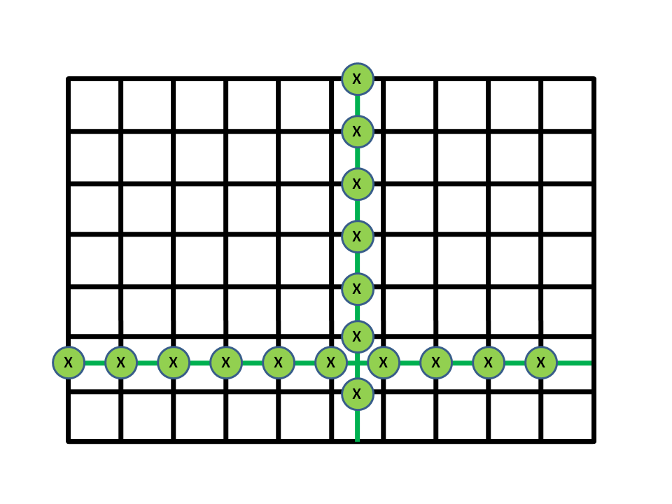
It has been observed in Verstraete that the equal superposition of the four logical states of the toric code |ψket𝜓|\psi\rangle has a PEPS representation with bond dimension 222. Since the logical X𝑋X in the first (resp. second) logical qubit is implemented by a non-contractible cut of σXsubscript𝜎𝑋\sigma_{X} operators along the vertical (resp. horizontal) direction Kitaev , |ψket𝜓|\psi\rangle remains invariant under these two “Wilson loops” (see fig. 15).
Refer to caption
Figure 15: “Wilson loops” that keep invariant the PEPS associated to the toric code.

We will see in this section how the existence of this kind of Wilson loops imply again that the PEPS cannot be injective.

Theorem 19.

Let |ψAketsubscript𝜓𝐴|\psi_{A}\rangle be PEPS in a L×N𝐿𝑁L\times N square lattice with local Hilbert space dimension d𝑑d such that there exists a uU(d)𝑢𝑈𝑑u\in U(d) with the properties:

  1. (i)

    uL𝟙rest|ψA=|ψAtensor-productsuperscript𝑢tensor-productabsent𝐿subscript1restketsubscript𝜓𝐴ketsubscript𝜓𝐴u^{\otimes L}\otimes\mathbbm{1}_{\text{rest}}|\psi_{A}\rangle=|\psi_{A}\rangle for a loop in the vertical direction.

  2. (ii)

    uN𝟙rest|ψA=|ψAtensor-productsuperscript𝑢tensor-productabsent𝑁subscript1restketsubscript𝜓𝐴ketsubscript𝜓𝐴u^{\otimes N}\otimes\mathbbm{1}_{\text{rest}}|\psi_{A}\rangle=|\psi_{A}\rangle for a loop in the horizontal direction.

  3. (iii)

    u𝟙rest|ψA|ψAtensor-product𝑢subscript1restketsubscript𝜓𝐴ketsubscript𝜓𝐴u\otimes\mathbbm{1}_{\text{rest}}|\psi_{A}\rangle\not=|\psi_{A}\rangle for u𝑢u acting on a single site.

Then |ψAketsubscript𝜓𝐴|\psi_{A}\rangle cannot be injective for any region of size L/5×N/5absent𝐿5𝑁5\leq L/5\times N/5.

Proof.

We assume injectivity for a region of size L/5×N/5𝐿5𝑁5L/5\times N/5, (i) and (ii) and will show that (iii) does not hold. By applying (i) to all columns and Theorem 13, we get that there exist unique Y𝑌Y and Z𝑍Z such that Fig. 11 holds. Applying now (i) to N/5𝑁5N/5 columns and injectivity we get that Y=𝟙𝑌1Y=\mathbbm{1} and applying (ii) to L/5𝐿5L/5 rows and injectivity we get that Z=𝟙𝑍1Z=\mathbbm{1}. So u𝟙rest|ψA=|ψAtensor-product𝑢subscript1restketsubscript𝜓𝐴ketsubscript𝜓𝐴u\otimes\mathbbm{1}_{\text{rest}}|\psi_{A}\rangle=|\psi_{A}\rangle for u𝑢u acting on a single site. ∎

VI Conclusions

In this work we have provided a simple characterization of the existence of symmetries in PEPS. The result is based on the proven existence of a “canonical form”. Since PEPS seem to give a fairly complete characterization of the low energy sector of local Hamiltonians, the result paves the way for a better understanding of the restrictions that symmetries impose on quantum systems. As a first example of the kind of results that one can obtain from this characterization, we have shown a 2D version of the Oshikawa-Yamanaka-Affleck extension for U(1)𝑈1U(1) of the Lieb-Schultz-Mattis theorem. We have also outlined, via the injectivity property, how three of the main indicators of topological order (degeneracy of the ground state, existence of Wilson loops and corrections to the area law) are related.

VII Acknowledgments

M. Sanz would like to thank the QCCC Program of the EliteNetzWerk Bayern as well as the DFG (FOR 635, MAP and NIM) for the support. D. Perez-Garcia and C. Gonzalez-Guillen acknowledge financial support from Spanish grants I-MATH, MTM2008-01366 and CCG08-UCM/ESP-4394 and M.M. Wolf acknowledges support by QUANTOP and the Danish Natural Science Research Council(FNU).

References

  • (1) A. Affleck, T. Kennedy, E. H. Lieb, and H. Tasaki, Commun. Math. Phys. 115, 477 (1988).
  • (2) F. Verstraete and J. I. Cirac (2004), cond-mat/0407066; F. Verstraete, V. Murg, and J. I. Cirac, Advances in Physics 57, 143 (2008); N. Maeshima, Y. Hieida, Y. Akutsu, T. Nishino, K. Okunishi, Phys. Rev. E 64 (2001) 016705; Y. Nishio, N. Maeshima, A. Gendiar, T. Nishino, cond-mat/0401115 (2004).
  • (3) M. B. Hastings, Phys. Rev. B 76, 035114 (2007); M. B. Hastings JSTAT, P08024 (2007); F. Verstraete, J.I. Cirac, Phys. Rev. B 73, 094423 (2006)
  • (4) F. Verstraete, M.M. Wolf, D. Pérez-García, Phys. Rev. Lett 96, 220601 (2006).
  • (5) O. Buerschaper, M. Aguado, G. Vidal, Phys. Rev. B 79, 085119 (2009)
  • (6) E. Rico, H.J. Briegel, Ann. of Phys. 323:2115-2131 (2008).
  • (7) D. Gross, J. Eisert, Phys. Rev. Lett. 98, 220503 (2007); D. Gross, J. Eisert, N. Schuch, D. Perez-Garcia, Phys. Rev. A 76, 052315 (2007)
  • (8) E. Lieb, T. Schultz and D. Mattis, Ann. Phys. 16, 407 (1961).
  • (9) M.B. Hastings, Phys.Rev. B69 (2004) 104431; B. Nachtergaele, R. Sims, Commun. Math. Phys. 276 (2007) 437–472.
  • (10) M. Oshikawa, M. Yamanaka and I. Affleck, Phys. Rev. Lett. 78, 1984 (1997).
  • (11) D. Pérez-García, M. M. Wolf, M. Sanz, F. Verstraete and J. I. Cirac, Phys. Rev. Lett. 100, 167202 (2008)
  • (12) F. Anfuso, A. Rosch Phys. Rev. B 76, 085124 (2007).
  • (13) M. Fannes, B. Nachtergaele and R. W. Werner, Comm. Math. Phys. 144, 443 (1992).
  • (14) D. Pérez-García, F. Verstraete, M.M. Wolf, J.I. Cirac, Quantum Inf. Comput. 7, 401 (2007).
  • (15) G. Vidal, Phys. Rev. Lett. 91, 147902 (2003).
  • (16) N. Schuch, M. M. Wolf, F. Verstraete, J. I. Cirac, Phys. Rev. Lett. 98, 140506 (2007)
  • (17) D. Pérez-García, F. Verstraete, J.I. Cirac and M.M. Wolf, Quant. Inf. Comp. 8, 0650-0663 (2008).
  • (18) R. A. Horn, C. R. Johnson, Topics in Matrix Analysis, Cambridge University Press 1991.
  • (19) S. Singh, R. N. C. Pfeifer, G. Vidal, arXiv:0907.2994.
  • (20) M. Sanz, M.M. Wolf, D. Pérez-García and J. I. Cirac, Phys. Rev. A 79, 042308 (2009)
  • (21) A. Yu. Kitaev, Annals Phys. 303 (2003) 2-30.