On the gravitational origin of the Pioneer Anomaly

Abstract

From Doppler tracking data and data on circular motion of astronomical objects we obtain a metric of the Pioneer Anomaly. The metric resolves the issue of manifest absence of anomaly acceleration in orbits of the outer planets and extra-Pluto objects of the Solar system. However, it turns out that the energy-momentum tensor of matter, which generates such a gravitational field in GR, violates energy dominance conditions. At the same time the equation of state derived from the energy-momentum tensor is that of dark energy with $w=-1/3$. So the model proposed must be carefully studied by ”Grand-Fit” investigations.

I Introduction

Spacecrafts Pioneer 10 and 11 were launched in the early 1970’s for the exploration of outer planets of the Solar system (see the special issue of Science 183, No. 4122, 25 January 1974, especially Soberman1974 ; Anderson1974 ). After the encounters with Jupiter and Saturn they followed hyperbolic trajectories on leaving the Solar system. Because of rotational spin-stabilization of these spacecrafts, which reduces the need for manoeuvres, they represent unique experiments for testing our understanding of celestial mechanics. The accuracy of acceleration measurements for the Pioneer spacecrafts is about $10^{-10}$ m/s² PioneerMissionPlan ; Scherer1997 .

During the flight spacecrafts were continuously tracked by Doppler effect on retransmitted radio signals. Then data were fitted to theoretical ones obtained in PPN approximation initially by ODP program of JPL (JPL’s Export Planetary Ephemeris DE405 was used for planet motion).

But surprisingly above 10 a.u. of heliocentric distance the systematical deviation of experimental and theoretical data was found Pioneer1998 . This deviation can be described simply as a constant acceleration towards the Sun with magnitude of about $8\cdot 10^{-10}$ m/s². This value is the same — within error limits — for all the spaceships Pioneer 10 and 11, Galileo and Ulysses and for all distances from the Sun Pioneer2001 .

This coincidence has been interpreted as a hint of the gravitational — metric — origin of the acceleration. But at the same time there are no signatures of such an acceleration in the orbits of outer planets and other objects in the Solar system. Inclusion of such acceleration leads to unavoidable deviations from the observed planet positions Pioneer2006 ; Iorio2007 .

Many attempts to explain the anomaly were made during last 10 years. Some of the recent work on this subject includes analyses of: the thermal radiation of the Pioneers ISI:000263816800017 ; ISI:000261214100012 , the gravitational attraction by the Kuiper Belt ISI:000238999400005 ; ISI:000239223200009 ; ISI:000232936700007 , the cosmological origin of the Anomaly ISI:000255093800006 ; ISI:000242327900022 ; ISI:000255524300012 ; ISI:000258636700088 ; ISI:000236229700005 ; ISI:000246464000017 , the influence of multipole moments of the Sun 2005AIPC..758..129Q , the clocks acceleration ISI:000227551100006 and many proposes of modified gravity ISI:000238120300014 ; ISI:000254557000003 ; ISI:000259935000020 ; ISI:000257329300072 including even laboratory investigations on very small acceleration dynamics ISI:000245691400011 and interesting endeavors to constrain some parameters of modified gravity theories by the known value of the Pioneer Anomaly ISI:000248810500006 ; ISI:000262356900001 .

In the frame of metric theories of gravitation there is an attractive possibility to explain the Pioneer Anomaly by metric perturbation, preserving at the same time the character of planet motion. It is possible because the Pioneers’ trajectories are very different from planet orbits: spacecrafts leave the Solar system almost in a radial direction, while planets orbit the Sun almost circularly. The potential possibility of such an approach was noted independently in a series of manuscripts 2005CQGra..22.2135J ; 2006CQGra..23..777J ; 2006CQGra..23.7561J , but authors of these works didn’t analyze the origin of the metric. Our approach is closer to that of Kjell Tangen Tangen2007 , but with more rigor because we don’t neglect perturbation of the space components of metric.

The goal of paper is to find the static space-time metric close to Schwarzschild one, in which radial motion of test bodies shows the Pioneer Anomaly, but circular motion doesn’t. For this purpose in section II we develop and discuss an algorithm of metric determination from data on radial and circular motions. Metric determination does not make use of Einstein equations so it is applicable to any pure metric theory of gravity in terminology of Will et. al. Will1993 ; Will2006 . Then we apply the method in the case of the Pioneer Anomaly, starting from the Schwarzschild space-time and recover the properties of matter forming such a metric within GR (section III). Finally some concluding remarks are made.

II Space-time determination from radial and circular motions

II.1 Metric choice and time definition

We begin with the interval with 3 metric functions $\tau$, $\rho$ and $\sigma$ (for simplicity it was taken $c=1$)

$$ds^{2}=e^{\tau(r)}dt^{2}-e^{\rho(r)}dr^{2}-e^{\sigma(r)}r^{2}(d\theta^{2}+\cos^{2}\theta d\varphi^{2}),$$ (1)

and then find the gauge relation between them for maximal simplification. The metric functions $\tau$, $\rho$ and $\sigma$ will be referred as time, radial and transverse metric function or coefficient, respectively. We consider radial and circular motions in such a space-time separately and find connections between metric functions following from the known properties of the motion. But first of all we must recall some time convention.

The metric (1) is written in the form that is consistent with global clock synchronization, in fact $\partial/\partial t$ being timelike Killing vector. So in the approach proposed when the cosmological effects is totally neglected and Solar system is supposed to be placed in a space-time, that is Minkowskian at spatial infinity, the coordinate time is the astronomical ephemerides time ET (up to a multiplier). This is the usual approximation used for PPN-ephemeride calculations.

There is a difficulty, because the perturbations required by the Pioneer Anomaly grow with the radial distance, so the perturbed space-time is not asymptotically flat. But it is not a big problem because before the metric perturbations grow significantly the space-time has a wide nearly-flat region in which we can choose almost Minkowskian observers and coordinates. So further if we talk about ”spatial infinity”, we mean this wide region, in the Solar system scale the effects of difference between this approximation and rigorous treatment are negligible. The same problem with the same solution is arising in the PPN-approximation then we must place the system not in Minkowskian background but in the cosmological one. Additionally, as it can be shown, in PPN-approach the cosmological effects, such as mutual acceleration of geodetically moving bodies, have the second order in $H$. Therefore even while the Pioneer Anomaly acceleration is nearly equal to $cH$, in the framework of pure metric theories of gravitation there is no possibility to link it to the cosmological expansion (early but almost exhaustive analysis of the problem was made by R. C. Tolman (Tolman, , §§153–156), for the recent work on subject see the articles mentioned in the Introduction and additionally FahrSiewert2006 ; MizonyLachiezeRey2005 ; Licht2001 and references within).

The radial coordinate rescaling $r\rightarrow f(r)$ changes all metric functions, giving a possibility to imply gauge conditions on the metric coefficients. But there are two invariants, i.e. physically measurable quantities, which characterize the distance from a given point to the center of space symmetry. Firstly it is an atomic time rate in comparison with the coordinate time rate (or atomic time rate on ”spatial infinity”) $e^{\tau/2}$, and secondly it is an area of a sphere of points equidistant to the center of the space $4\pi r^{2}e^{\sigma}$. So the numerical values of time and transverse metric coefficients have clear physical meaning for a given space-time point and only $\rho(r)$ can take arbitrary values. Usual choices include $\rho\equiv\sigma$ corresponding to isotropic coordinates of PPN-approximation and implicit on $\rho(r)$ relation $\sigma\equiv 0$ corresponding to Schwarzschild coordinates.

II.2 Radial motion and its description by Doppler radio tracking

Radial motion in the space-time is fully described by the energy $g_{tt}\frac{dt}{ds}=e^{\tau(r)}u^{0}=k=const$ and the 4-velocity length conservation $e^{\tau(r)}u^{0^{2}}-e^{\rho(r)}u^{1^{2}}=\varepsilon,\ \varepsilon=0$ or 1 for electromagnetic waves and test bodies, respectively:

$$\frac{dt}{dr}=\frac{e^{\frac{\rho(r)-\tau(r)}{2}}}{\sqrt{1-\varepsilon e^{\tau(r)}/k^{2}}},$$ (2)

the constant $k$ being connected with the velocity $v$ of the spacecraft on ”space infinity”

$$k^{2}=\frac{1}{1-v^{2}}.$$ (3)

The relation (2) can be integrated to give us $t(r)$ dependence which in turn can be inverted giving $r(t)$. But there is a gauge freedom in the result because we can choose $\rho(r)$ freely. Moreover, this relation essentially involve both physical $\tau$ and unphysical $\rho$.

Our goal is to determine the metric functions from observations. Direct results of experimentation in astronomy and cosmology are the measurements of externally originated signals received on the world line of an observer. These signals have mostly electromagnetic character and can originate from some external source (e. g. the light emitted by the Sun and reflected by a planet) or be emitted by the observer him/herself and then returned to him/her after some interaction with outer bodies (as in case of radar measurements). The latter case is considered here as corresponding to the real situation Pioneer2001 .

The scheme of Doppler tracking used in the Pioneer experiments is very simple conceptually: an electromagnetic signal, emitted from the world line of the observer, is reflected back by the mirror on the world line of the spacecraft and then compared with the initial one again on the observer world line. To be more precise, the monochromatic electromagnetic signal, obtained from the high precision hydrogen maser (Pioneer2001, , subsection III.A), is emitted by the antennae on Earth in the direction of the spacecraft. This signal is detected by the spacecraft, amplified and reemitted back to Earth, where the measured waveform of arrived signal is compared with the emitted one to obtain the red shift of the signal and the time of signal travel (the very detailed description of the process can be found in Pioneer2001 ).

Now we must describe the Doppler tracking and the signal time arrival analysis in this space-time. In the geometric optics approximation (which is applicable for the case considered) the Doppler shift is governed simply by the ratio between scalar products of the 4-velocity on world lines and the null wave vector of the signal, parallel transported along the null geodesic line between emitter and receiver:

$$\frac{\nu_{r}}{\nu_{e}}=\frac{s_{e}}{s_{r}}=\frac{\vec{\mathstrut u}_{r}\cdot\vec{k}_{r}}{\vec{\mathstrut u}_{e}\cdot\vec{k}_{e}},$$ (4)

where $\nu_{r}$ and $\nu_{e}$ are received and emitted frequencies, measured by the standard atomic clocks,
$s_{r}$ and $s_{e}$ are proper times of one cycle of oscillation,
$u_{r}$ and $u_{e}$ are 4-velocities of receiver and emitter,
$k_{r}$ and $k_{e}$ are tangential null vectors (wave vector), parallel transported along the path of the signal.

Atomic clock time deviations from ephemerides time along with all known effects of Earth motion were taken into account during the data processing (see Pioneer2001 ), so for the description of such a small deviation like the Pioneer Anomaly it is sufficient to use the simple model, in which the emitter of the initial signal and the receiver of the retranslated signal are fixed at constant distances from the Sun on the line from the Sun to apparatus. The signal is emitted from this ”fixed” Earth at $r_{0}$ and $t-t_{p}$, received by the spaceship at $r$ and $t$, amplified, exactly retransmitted back to Earth and finally compared with the initial frequency on the ”fixed” Earth again at $r_{0}$ and $t+t_{p}$ ($t_{p}$ is the time of signal propagation, the same for forward and backward directions).

As it can be shown easily, the frequency $\nu_{r}$ received on Earth is connected to the initially emitted $\nu_{e}$ as

$$\nu_{r}=\nu_{e}\frac{1-\sqrt{1-e^{\tau(r)}/k^{2}}}{1+\sqrt{1-e^{\tau(r)}/k^{2}}}.$$ (5)

This expression can be readily reduced to special relativistic one in the case of $e^{\tau}\equiv 1$.

As a relation between physical quantities only, this equation does not involve arbitrary unphysical $\rho$ function. The problem of gauge choice comes with the definition of $r(t)$: from (5) one can determine $e^{\tau(r(t))}$, but because the radial coordinate $r$ (and consequently $r(t)$) is arbitrary, the radial dependence of the time metric coefficient remains gauge dependent. It is interesting also that this relation cannot be represented by a power series in terms of small deviations of $e^{\tau(r)}$ and $k$ from 1. The transverse space metric coefficient $\sigma(r)$ naturally cannot be determined from the radial motion only.

So we come to an unavoidable alternative of a-priory $r(t)$ definition or a-priory imposing some gauge condition on $\rho(r)$. In each case the remaining function is defined by the experimental data, and our goal now is to find in which case the process of metric restoration can be done without unnecessary complications. In the next subsection we consider these possibilities in some details and then show that the best choice is the latter case, i.e. imposing a gauge.

II.3 General formulae and coordinate choice

While the time of signal arrival to the spaceship $t$ can be easily determined as a half-sum of observed times of emitting $t_{e}$ and receiving $t_{r}$ of the signal at the ”fixed” Earth

$$t=\frac{t_{r}+t_{e}}{2},$$ (6)

the corresponding $r$ determination is not so trivial task. In general we can measure only the time of signal travel from the ”fixed” Earth to the spaceship as a half-difference between observed times of sending and receiving of the signal

$$t_{p}=\int_{r_{0}}^{r}{e^{\frac{\rho(r)-\tau(r)}{2}}}\,dr=\frac{t_{r}-t_{e}}{2}.$$ (7)

These are results of a different method of tracking — signal time arrival analysis, which in essence represents integration of the Doppler data.

So to recover $\rho(r)$ from a given $r(t)$ we must firstly find $\tau(r)$ by (5) from the observed redshift, and then solve an integral equation above. On the other hand, to find $r(t)$ from a given $\rho(r)$ it is sufficient to solve a non-integral equation following from relation (2) for the spacecraft motion

$$\int_{t_{0}}^{t}e^{\frac{\tau(r(t))}{2}}\sqrt{1-e^{\tau(r(t))}/k^{2}}\,dt=\int_{r_{0}}^{r}{e^{\frac{\rho(r)}{2}}}\,dr,$$ (8)

where $t_{0}$ is the time when the spacecraft leaves ”fixed” Earth. The left-hand side of the relation can be found totally from the observed frequency shifts by (5), and the right-hand side is a known function of $r$ with given $\rho(r)$.

Consequently maximal simplification of the problem is reached in the case of a-priory given radial metric function $\rho(r)$. It is nonsense to define it dependent on still unknown time and transverse metric functions, with one interesting exclusion: if $\tau(r)\equiv\rho(r)$ then $r(t)$ can be recovered from (7) simply as

$$r=r_{0}+\frac{t_{r}-t_{e}}{2}.$$ (9)

This choice of coordinates known as light or null coordinates is not so usual as Schwarzschild ($\sigma\equiv 0$) or isotropic ($\rho\equiv\sigma$) coordinates but it is the most suitable one for the situation. Both abovementioned choices are especially inappropriate here because they rely on transversal metric function that does not reveal itself in pure radial motions.

II.4 Circular motion

We know that the near-circular motion of outer Solar system objects (i.e. Neptune or Pluto) is unperturbed by the Pioneer Anomaly acceleration Pioneer2006 ; Iorio2007 . This gives us a way to determine the transversal metric coefficient and therefore to find metric completely.

The angular velocity of circular motion ($\theta=0,\ \phi=\omega t$) in the considered space-time is defined by the ratio of derivatives of time and transversal space metric coefficients

$$\omega^{2}(r)=\frac{(e^{\tau(r)})^{\prime}}{(r^{2}e^{\sigma(r)})^{\prime}}=\frac{(e^{\tau(r(t))}){}\dot{}}{(r^{2}e^{\sigma(r(t))}){}\dot{}},$$ (10)

where as usual prime denotes differentiation with respect to radial coordinate, and dot denotes differentiation in time. So there is no dependence on the radial metric part at all. Moreover as $\omega(r(t))$ and $(e^{\tau(r(t))}){}\dot{}$ is directly observable, so the transverse metric coefficient $r^{2}e^{\sigma(r(t))}$ can be obtained by a simple integration without any notion of the radial metric function.

So again recalling the radial motion equation (2) we conclude that all gauge conditions for $\rho(r)$ involving transverse metric coefficient are not convenient for treatment of the Pioneer Anomaly, because all such conditions lead to coupling of equations (5) and (10) which can be solved independently otherwise.

II.5 Final list of relations and concluding remarks

So we work in light or null coordinates $\tau(r)\equiv\rho(r)$, then:

$$\frac{dt}{dr}=\frac{1}{\sqrt{1-\varepsilon e^{\tau(r)}/k^{2}}}.$$ (11)

The trajectory of the spacecraft $$r(t) t_{e} t_{r}$$ is recovered simply from time of sending and arrival of signal

$$t_{p}=r-r_{0}\quad\Rightarrow\quad t=\frac{t_{r}+t_{e}}{2},\qquad r=r_{0}+\frac{t_{r}-t_{e}}{2},$$ (12)

and the observed redshift of the signal

$$z(t)=\frac{\nu_{e}-\nu_{r}}{\nu_{e}}=\frac{\Delta\nu}{\nu_{e}}=\frac{2}{(1-e^{\tau(r(t))}/k^{2})^{-1/2}+1},$$ (13)

can be immediately transformed into time metric coefficient

$$e^{\tau(r(t))}=k^{2}\left[1-\left(\frac{z(t)}{2-z(t)}\right)^{2}\right]=4k^{2}\frac{(1-z)}{(2-z)^{2}}.$$ (14)

The transverse space metric coefficient is defined by the dependence of angular velocity $\omega$ on radial coordinate $r$

$$r^{2}e^{\sigma(r)}=r_{0}^{2}e^{\sigma(r_{0})}-\int_{r_{0}}^{r}\frac{4k^{2}z(r)z^{\prime}(r)}{(2-z(r))^{3}\omega^{2}(r)}dr,$$ (15)

which for the space-time of the Pioneer Anomaly should be the same as in the Schwarzshild field (or very close to it). So basing on the Schwarzshild metric one can find such perturbations of metric coefficients, that the circular motion remains unperturbed, but the radial one shows small deviation — the Pioneer Anomaly.

It is worth noting that the sentence ”the circular motion remains unperturbed” denotes exactly the following: if, neglecting all mutual planet disturbances, the period of circularly orbiting planet will be measured in the units of ephemerides time and the distance of planet from the baricenter of the Solar system will be found by analyzing light propagation times on straight lines from the Sun (null coordinates!) then the values of the period and the distance will exactly be the same as needed for the 3rd Kepler law to hold — exactly as in the Schwarzshild field.

III The Pioneer Anomaly and its source in GR

III.1 Schwarzschild space-time in light coordinates

Radius $r$ in light coordinates of the Schwarzschild field is related to the usual Schwarzschild radial coordinate $r_{s}$ as

$$r=r_{s}+r_{g}\ln\left(\frac{r_{s}}{r_{g}}-1\right),\quad r_{s}=r_{g}\left(1+\mathop{W}\left(e^{\frac{r}{r_{g}}-1}\right)\right).$$ (16)

The interval in null coordinates is as follows

$$\begin{split}ds^{2}=&\frac{\mathop{W}\left(e^{\frac{r}{r_{g}}-1}\right)}{1+\mathop{W}\left(e^{\frac{r}{r_{g}}-1}\right)}(dt^{2}-dr^{2})\\ &-r_{g}^{2}\left(1+\mathop{W}\left(e^{\frac{r}{r_{g}}-1}\right)\right)^{2}(d\theta^{2}+\cos^{2}\theta d\varphi^{2}),\end{split}$$ (17)

so that

$$e^{\tau(r)}=e^{\rho(r)}=\frac{\mathop{W}\left(e^{\frac{r}{r_{g}}-1}\right)}{1+\mathop{W}\left(e^{\frac{r}{r_{g}}-1}\right)}=r_{g}\mathop{W}\nolimits^{\prime}_{r}\left(e^{\frac{r}{r_{g}}-1}\right),$$ (18)

$$e^{\sigma(r)}=\frac{r_{g}^{2}}{r^{2}}\left(1+\mathop{W}\left(e^{\frac{r}{r_{g}}-1}\right)\right)^{2},$$ (19)

where $$W(x) W$$ is the so called multiplicative logarithm or Lambert function

$$W(x)e^{W(x)}=x.$$ (20)

III.2 The Pioneer Anomaly. Radial perturbation

The Pioneer Anomaly is the linear in ephemerides time ET deviation of the experimentally obtained frequency of received signal $\nu_{r}$ from the ”modelled” one $\nu_{m}$

$$\frac{d}{d\text{{ET}}}(\nu_{r}-\nu_{m})=-\nu_{e}\frac{2a_{P}}{c},$$ (21)

where $a_{P}\sim 8\cdot 10^{-10}\ \mbox{m/s}^{2}$ is the ”unmodelled” acceleration Pioneer2001 . The ephemerides time coincides with time coordinate $t$ of the metric considered (as described earlier). For the most part of range of the Pioneer Anomaly found (from $\sim 15$ to $\sim 80$ a.u.) the deviation of the Pioneers’ orbits from pure radial motion is comparable to or even below experimental uncertainty in the acceleration: it can be estimated roughly as a ratio of the semi-major axis $a$ absolute value to heliocentric distance $r$

$$\frac{|a|}{r}\lesssim\frac{10^{9}\text{km}}{40\cdot 150\cdot 10^{6}\text{km}}\simeq 17\%,$$ (22)

while experimental error in the acceleration is $1.33/8.74\simeq 15\%$ (see Appendix of Pioneer2001 ). It should be noted that this uncertainty prevents Anderson et. al. from determining the direction of the acceleration: to Earth or to the Sun (see beginning of section VII and especially note 73 of Pioneer2001 ).

The modelled frequency and velocity of the spacecraft are

$$\nu_{m}=\nu_{0}\;\frac{1+\frac{1}{W(e^{\frac{r}{r_{g}}-1})}}{1-v^{2}}\left(1-\sqrt{1-\frac{1-v^{2}}{1+\frac{1}{W(e^{\frac{r}{r_{g}}-1})}}}\right)^{2},$$ (23)

$$\left(\frac{dr}{dt}\right)_{m}=v_{m}(r)=\sqrt{\frac{v^{2}+1/W(e^{\frac{r}{r_{g}}-1})}{1+1/W(e^{\frac{r}{r_{g}}-1})}},$$ (24)

so accurately expanding the expression (14) for the time metric coefficient from the red shift $z(r(t))$, one can find that given the accuracy of the Pioneer Anomaly measurements one can simply use the relation

$$\delta e^{\tau(r)}\simeq-\frac{z(r)\;\delta z(r)}{2}=a_{P}\;z(r)\Delta t(r),$$ (25)

where $\Delta t=t(r)-t_{0}$ is the time from the start of the Pioneer Anomaly (we suppose that for $r<r_{0}$ the metric coincides with the Schwarzschild one, so before $t_{0}=t(r_{0})$ there is no anomalous acceleration), $\delta z(r)$ is a deviation of observed red shift from the modelled one.

In the first approximation $t(r)$ dependence can be replaced with the ”modelled” time, which to the accuracy of the measurements is the same as in the Newtonian case

$$t_{m}(r)=t(r_{0})+\int_{r_{0}}^{r}\frac{dr}{\dot{r}}\simeq\\ \simeq t_{0}+\frac{r}{v^{2}}\sqrt{v^{2}+\frac{r_{g}}{r}}-\frac{r_{g}}{v^{3}}\sinh^{-1}\left(\sqrt{\frac{r}{r_{g}}}v\right).$$ (26)

Finally inserting this and modelled $z(r)$ into the equation (25) we arrive to the perturbation of the time metric coefficient

$$\delta e^{\tau(r)}=2a_{P}\Biggl{(}r-C\sqrt{v^{2}+\frac{r_{g}}{r}}+\\ +\frac{r_{g}}{v^{2}}\left[1-\sqrt{1+\frac{r_{g}}{r\;v^{2}}}\sinh^{-1}\left(\sqrt{\frac{r}{r_{g}}}v\right)\right]\Biggr{)},$$ (27)

where $C$ is a constant which can be determined from $r_{0}$ and $v$. The perturbation appears to be non-linear in $r$, but for the Pioneer 10/11 parameters the deviation from linearity is buried deep in the experimental errors. It is illustrated by the figure 1, which shows the deviation of the time metric coefficient compared to the ”naive” post-Newtonian approach, where one simply adds to the gravitational potential $\Phi(r)$ a term linear in radius and use $e^{\tau(r)}\simeq 1+\Phi(r)$. As we can see, the difference is mainly in the slope, all the graphs are nearly linear. Moreover, the relative value of the deviation from linearity is decreasing with radial distance. So the linear approximation $\delta e^{\tau(r)}\simeq 2\eta a_{P}(r-r_{0})$ is sufficient for the Pioneer Anomaly explanation. The only difference between this more accurate result and the ”naive” post-Newtonian one is the presence of $\eta$, which is always less then 1 (see table 1).

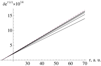
Figure 1: Metric perturbation $\delta e^{\tau(r)}$ of the Pioneer Anomaly for $v$ from 5 km/s to 50 km/s in 5 km/s steps (solid lines from bottom to top) for the metric matching the Schwarzschild metric at 12 a. u., compared to the ”naive” post-Newtonian one (dashed line)

Table 1: The quantity $1-\eta$ of the best linear approximations $\delta e^{\tau(r)}\simeq 2\eta a_{P}(r-r_{0})$ on the interval $r_{0}\leq r\leq 70$ a. u. for different velocities $v$ and metric matching distances $r_{0}{}^{*}$

$r_{0}$, a. u.	$v$, km/s
	5	10	15	20	25	30	35	40	45	50
10	0.175	0.098	0.057	0.036	0.025	0.018	0.013	0.010	0.008	0.007
15	0.146	0.077	0.044	0.027	0.018	0.013	0.010	0.008	0.006	0.005
20	0.122	0.062	0.034	0.021	0.014	0.010	0.007	0.006	0.005	0.004
∗ $r_{0}$ is the radial coordinate at which the metric coefficients coincides with the Schwarzschild ones.

III.3 Transversal perturbation leaving planet orbits unchanged. Necessity of the central source

Now we assume that in the perturbed space-time planets orbit with the same periods as in the unperturbed Schwarzschild solution, so that there is no signatures of the Pioneer acceleration in the orbits of planets. So the angular velocity dependence $\omega(r)$ must be the same as in the Schwarzschild case (see, e. g., eq. (25.40) of MTW )

$$\omega_{s}^{2}(r)=\frac{{e^{\tau(r)}}^{\prime}}{(r^{2}e^{\sigma(r)})^{\prime}}=\frac{1}{2r_{g}^{2}\left(1+\mathop{W}\left(e^{\frac{r}{r_{g}}-1}\right)\right)^{3}}=\frac{r_{g}}{2r_{s}^{3}},$$ (28)

and the perturbation in $e^{\tau}$ must lead to such a perturbation in $r^{2}e^{\sigma}$ that $\omega^{2}(r)$ remains invariant. In the perturbed space-time by the general formula (10) we have from simple mathematics

$$\omega_{s}^{2}(r)=\frac{{e^{\tau(r)}}^{\prime}}{(r^{2}e^{\sigma(r)})^{\prime}}=\omega^{2}(r)=\frac{(e^{\tau(r)}+\delta e^{\tau(r)})^{\prime}}{(r^{2}e^{\sigma(r)}+\delta(r^{2}e^{\sigma(r)}))^{\prime}}=\\ =\frac{(e^{\tau(r)})^{\prime}+(\delta e^{\tau(r)})^{\prime}}{(r^{2}e^{\sigma(r)})^{\prime}+(\delta(r^{2}e^{\sigma(r)}))^{\prime}}=\frac{(\delta e^{\tau(r)})^{\prime}}{(\delta(r^{2}e^{\sigma(r)}))^{\prime}}.$$ (29)

So the perturbation of the transverse metric coefficient is

$$\delta(r^{2}e^{\sigma(r)})=r^{2}\delta e^{\sigma(r)}=\int_{r_{0}}^{r}\omega^{-2}(r)\delta({e^{\tau(r)}})^{\prime}\,dr,$$ (30)

and finally

$$\delta e^{\sigma(r)}=\frac{4a_{P}\eta\,r_{g}^{2}}{r^{2}}\int_{r_{0}}^{r}\left(1+\mathop{W}\left(e^{\frac{r}{r_{g}}-1}\right)\right)^{3}\,dr\simeq\\ \simeq\frac{4a_{P}\eta\,r_{g}^{2}}{r^{2}}\int_{r_{0}}^{r}\left(\frac{r}{r_{g}}\right)^{3}dr=\frac{4a_{P}\eta(r^{4}-r_{0}^{4})}{r^{2}r_{g}}.$$ (31)

In the first approximation the perturbation of $r^{2}e^{\sigma(r)}$ grows quartically in radius.

Note the gravitational radius of the source $r_{g}$ in the answer. So the effect of the Pioneer Anomaly can be reproduced only by perturbations of Schwarzschild space-time and not Minkowski one. So the gravitational explanation of the Pioneer Anomaly can be obtained without the equivalence principle violation required by various authors Pioneer2006 ; Iorio2007 ; Tangen2007 .

III.4 Matter corresponding to the obtained metric in General Relativity

One can try to find the gravitational field theory, that gives equations of the gravitational field allowing the solution found for the weak field of a point mass. But we think that it is not very promising because there are no reliable experimental evidence in favor of any gravitational theory other than General Relativity.

Instead we find the properties of matter surrounding the point mass in GR that can generate the obtained metric. Because in the scale of Solar system experiments the influence of cosmological constant is negligible, for the determination of matter one can use the Einstein equations of the form

$$G_{ij}=R_{ij}-\frac{1}{2}Rg_{ij}=\kappa T_{ij},\qquad\kappa=\frac{8\pi G}{c^{4}}.$$ (32)

Using for simplicity the metric in the form

$$ds^{2}=e^{\tau(r)}dt^{2}-e^{\rho(r)}dr^{2}-e^{\sigma(r)}(d\theta^{2}+\sin^{2}\theta d\phi^{2}),$$ (33)

one arrives at the Einstein tensor

$$G_{ij}=\frac{e^{-\rho}}{4}\Bigl{(}\lambda_{t}T_{i}\otimes T_{j}-\lambda_{s}S_{i}\otimes S_{j}-\lambda g_{ij}\Bigr{)},$$ (34)

$$S_{i}=\Bigl{\{}0,e^{\frac{\rho}{2}},0,0\Bigr{\}},\qquad T_{i}=\Bigl{\{}e^{\frac{\tau}{2}},0,0,0\Bigr{\}},$$ (35)

$$-S_{i}S^{i}=T_{i}T^{i}=1,\qquad S^{i}T_{i}=0,$$ (36)

$$\lambda_{t}=4e^{\rho-\sigma}+\left(\rho^{\prime}-2\sigma^{\prime}-\tau^{\prime}\right)\left(\sigma^{\prime}-\tau^{\prime}\right)+2\left(\tau^{\prime\prime}-\sigma^{\prime\prime}\right),$$ (37)

$$\lambda_{s}=4e^{\rho-\sigma}-\tau^{\prime}\left(\sigma^{\prime}-\tau^{\prime}\right)-\rho^{\prime}\left(\sigma^{\prime}+\tau^{\prime}\right)+2\left(\tau^{\prime\prime}+\sigma^{\prime\prime}\right),$$ (38)

$$\lambda=\sigma^{\prime 2}+\sigma^{\prime}\tau^{\prime}+\tau^{\prime 2}-\rho^{\prime}\left(\sigma^{\prime}+\tau^{\prime}\right)+2\left(\tau^{\prime\prime}+\sigma^{\prime\prime}\right).$$ (39)

Expanding to the first power of $a_{P}$ one obtains

$$\lambda_{t}=-96\,\frac{a_{P}\eta}{r_{g}},\quad\lambda_{s}=-32\,\frac{a_{P}\eta}{r_{g}}\,\frac{r_{0}^{4}}{r^{4}},$$

$$\lambda=16\,\frac{a_{P}\eta}{r_{g}}\left(3-\frac{r_{0}^{4}}{r^{4}}\right).$$ (40)

The algebraic type of the energy-momentum tensor at spatial infinity is that of an ideal fluid (by $\lambda_{s}\rightarrow 0$) with constant positive pressure

$$p=\frac{e^{-\tau}}{4\kappa}\lambda\rightarrow 12\,\frac{a_{P}\eta}{\kappa r_{g}}>0,$$ (41)

but negative energy density

$${\rho=\frac{e^{-\tau}}{4\kappa}(\lambda_{t}-\lambda)\rightarrow-36\,\frac{a_{P}\eta}{\kappa r_{g}}<0.}$$ (42)

It is worth noting that relation between $p$ and $\rho$ is as for an ultrarelativistic fluid except for the sign: instead of $p=\rho/3$ one has asymptotically $p=-\rho/3$. This is a typical equation of state of dark energy with parameter $w=-1/3$. It is interesting that such a fluid does not change the cosmological dynamics of Friedman-Lemaître universe (see, e.g., (PeeblesRatra2003, , III.E)).

IV Conclusions

In this work we show that it is possible to perturb time metric coefficient of the Schwarzschild space-time in such a way that the Pioneer Anomaly is reproduced. Moreover, because planet motion is governed also by anther component of the metric, we can tune it so that circular orbits is not disturbed. This result applies in any pure metric theory of gravitation where test bodies follow geodetics of the metric. It is deduced that the perturbation of the time metric coefficient can be taken linear in $r$ without contradiction with the accuracy of experimental data obtained up to now.

Assuming the validity of the General Relativity, we find out the energy-momentum tensor generating the metric obtained. The tensor corresponds to an ideal fluid, however having negative energy density. It is interesting to note that an exact static solution with spherical symmetry is known for the ”fluid” with $3p+\rho=0$ (StanjukovichMel'nikov1983, , §8.5). This ”fluid” does not interact with the ordinary matter besides its gravitational influence on the metric, so it much like WIMPs or scalar field of gravitational theories of Brans-Dicke type. Thus the ordinary matter including spacecrafts and planets is moving geodesically.

Naturally the found ”fluid” does change the planet orbits (if they are not strictly circular) and light rays paths. The model proposed must be carefully studied in view of the ”Grand-Fit” investigations Pitjeva2005 ; 2008AIPC..977..254S , but direct measurements from the planned missions for testing General Relativity in space are preferable 2007arXiv0711.0304W ; 2005gr.qc…..6104L ; 2005gr.qc…..6139T . The absolute value of effects for the perturbation found as well as for exact solution of Stanjukovich and Ivanov will be studied in the forthcoming paper.

The analysis presented in this paper can encourage someone to find out which of the known alternatives to GR can reproduce the metric found or to invent some new theory which can do it. It is possible, but in our opinion the Pioneer Anomaly has some simple explanation by conventional and non-gravitational physics, which is not found yet. So the question of deep theoretical grounds for the existence of the ”fluid” in GR or of development of some new theory of gravitation based on the metric obtained is not in the scope of our article. Instead we point out that negative energy density of the ”fluid” is in a direct contradiction with the properties of conventional matter. One interesting possibility for the ”fluid” is dark energy, which has the right equation of state. Therefore we suppose that at present the metric (gravitational) origin of the Pioneer Anomaly cannot be ruled out.

- (1) R.K. Soberman, S.L. Neste, K. Lichtenfeld, Science 183(4122), 320 (1974)
- (2) J.D. Anderson, G.W. Null, S.K. Wong, Science 183(4122), 322 (1974)
- (3) Pioneer Extended Mission Plan, Revised, NASA/ARC document No. PC-1001 (NASA, Washington, D.C., 1994)
- (4) K. Scherer, H. Fichtner, J.D. Anderson, E.L. Lau, Science 278, 1919 (1997)
- (5) J.D. Anderson, P.A. Laing, E.L. Lau, A.S. Liu, M.M. Nieto, S.G. Turyshev, Physical Review Letters 81(14), 2858 (1998). DOI 10.1103/PhysRevLett.81.2858
- (6) J.D. Anderson, P.A. Laing, E.L. Lau, A.S. Liu, M.M. Nieto, S.G. Turyshev, Physical Review D 65(8), 082004 (2002). DOI 10.1103/PhysRevD.65.082004
- (7) L. Iorio, G. Giudice, New Astronomy 11(8), 600 (2006). DOI 10.1016/j.newast.2006.04.001
- (8) L. Iorio, Foundations of Physics 37(6), 897 918 (2007)
- (9) V.T. Toth, S.G. Turyshev, Physical Review D 79(4), 043011 (2009). DOI 10.1103/PhysRevD.79.043011
- (10) O. Bertolami, F. Francisco, P.J.S. Gil, J. Paramos, Physical Review D 78(10), 103001 (2008). DOI 10.1103/PhysRevD.78.103001
- (11) O. Bertolami, P. Vieira, Classical and Quantum Gravity 23(14), 4625 (2006). DOI 10.1088/0264-9381/23/14/005
- (12) J.A. De Diego, D. Nunez, J. Zavala, International Journal of Modern Physics D 15(4), 533 (2006). ArXiv:astro-ph/0503368
- (13) M. Nieto, Physical Review D 72(8), 083004 (2005). DOI 10.1103/PhysRevD.72.083004
- (14) H.J. Fahr, M. Siewert, Naturwissenschaften 95(5), 413 (2008). DOI 10.1007/s00114-007-0340-1
- (15) M. Carrera, D. Giulini, Classical and Quantum Gravity 23(24), 7483 (2006). DOI 10.1088/0264-9381/23/24/019
- (16) E. Hackmann, C. Lämmerzahl, Physical Review Letters 100(17), 171101 (2008). DOI 10.1103/PhysRevLett.100.171101
- (17) E. Hackmann, C. Lämmerzahl, Physical Review D 78(2), 024035 (2008). DOI 10.1103/PhysRevD.78.024035
- (18) V. Kagramanova, J. Kunz, C. Lämmerzahl, Physics Letters B 634(5-6), 465 (2006). DOI 10.1016/j.physletb.2006.01.069
- (19) M. Lachieze-Rey, Classical and Quantum Gravity 24(10), 2735 (2007). DOI 10.1088/0264-9381/24/10/016
- (20) H. Quevedo, in Gravitation and Cosmology, American Institute of Physics Conference Series, vol. 758, ed. by A. Macias, C. Lämmerzahl, D. Nunez (2005), American Institute of Physics Conference Series, vol. 758, pp. 129–136. DOI 10.1063/1.1900512. ArXiv:gr-qc/0506139v1
- (21) A. Ranada, Foundations of Physics 34(12), 1955 (2004). DOI 10.1007/s10701-004-1629-y
- (22) J. Brownstein, J. Moffat, Classical and Quantum Gravity 23(10), 3427 (2006). DOI 10.1088/0264-9381/23/10/013
- (23) H. Asada, Physics Letters B 661(2-3), 78 (2008). DOI 10.1016/j.physletb.2008.02.006
- (24) C. Massa, Astrophysics and Space Science 317(1-2), 139 (2008). DOI 10.1007/s10509-008-9862-z
- (25) R. Saffari, S. Rahvar, Physical Review D 77(10), 104028 (2008). DOI 10.1103/PhysRevD.77.104028
- (26) J.H. Gundlach, S. Schlamminger, C.D. Spitzer, K.Y. Choi, B.A. Woodahl, J.J. Coy, E. Fischbach, Physical Review Letters 98(15), 150801 (2007). DOI 10.1103/PhysRevLett.98.150801
- (27) G. Allemandi, M.L. Ruggiero, General Relativity and Gravitation 39(9), 1381 (2007). DOI 10.1007/s10714-007-0441-3
- (28) Q. Exirifard, Classical and Quantum Gravity 26(2), 025001 (2009). DOI 10.1088/0264-9381/26/2/025001
- (29) M.T. Jaekel, S. Reynaud, Classical and Quantum Gravity 22(11), 2135 (2005). DOI 10.1088/0264-9381/22/11/015
- (30) M.T. Jaekel, S. Reynaud, Classical and Quantum Gravity 23(3), 777 (2006). DOI 10.1088/0264-9381/23/3/015
- (31) M.T. Jaekel, S. Reynaud, Classical and Quantum Gravity 23(24), 7561 (2006). DOI 10.1088/0264-9381/23/24/025
- (32) K. Tangen, Physical Review D 76(4), 042005 (2007). DOI 10.1103/PhysRevD.76.042005.
- (33) C.M. Will, Theory and experiment in gravitational physics, edn. (Cambridge University Press, Cambridge, U.K.; New York, U.S.A., 1993)
- (34) C.M. Will, Living Reviews in Relativity 9(3), 1 (2006). Mode of access: http://www.livingreviews.org/lrr-2006-3. — Date of access: 22.05.2006.
- (35) R.C. Tolman, Relativity, thermodynamics and cosmology (Oxford, Clarendon Press, 1934)
- (36) H.J. Fahr, M. Siewert, ArXiv General Relativity and Quantum Cosmology e-prints arXiv:gr–qc/0610034v1 (2006)
- (37) M. Mizony, M. Lachieze-Rey, Astronomy and Astrophysics 434, 45 (2005). DOI 10.1051/0004-6361:20042195
- (38) A.L. Licht, ArXiv General Relativity and Quantum Cosmology e-prints arXiv:gr-qc/0102103v1 (2001)
- (39) C. Misner, K. Thorne, J. Wheeler, Gravitation (W.H. Freeman, San Francisco, U.S.A., 1973)
- (40) P.J.E. Peebles, B. Ratra, RMP 75(2), 559 (2003). DOI 10.1103/RevModPhys.75.559. arXiv:astro-ph/0207347v1
- (41) K.P. Stanjukovich, V.N. Mel’nikov, Hydrodynamics, fields and constants in the gravitational theory (E’nergoatomizdat, 1983). (in Russian)
- (42) E.V. Pitjeva, Astronomy Letters 31(3), 340 (2005)
- (43) E.M. Standish, in American Institute of Physics Conference Series, American Institute of Physics Conference Series, vol. 977 (2008), pp. 254–263. DOI 10.1063/1.2902789
- (44) SAGAS Collaboration, ArXiv e-prints arXiv:0711.0304v3 [gr-qc] (2007)
- (45) LATOR Collaboration, ArXiv General Relativity and Quantum Cosmology e-prints arXiv:gr-qc/0506104v3 (2005)
- (46) The Pioneer Explorer Collaboration, ArXiv General Relativity and Quantum Cosmology e-prints arXiv:gr-qc/0506139v1 (2005)