Passive scheme analysis for solving untrusted source problem in quantum key distribution

Abstract

As a practical method, the passive scheme is useful to monitor the photon statistics of an untrusted source in a Plug & Play quantum key distribution (QKD) system. In a passive scheme, three kinds of monitor mode can be adopted: average photon number (APN) monitor, photon number analyzer (PNA), and photon number distribution (PND) monitor. In this paper, the security analysis is rigorously given for the APN monitor, while for the PNA, the analysis, including statistical fluctuation and random noise, is addressed with a confidence level. The results show that the PNA can achieve better performance than the APN monitor and can asymptotically approach the theoretical limit of the PND monitor. Also, the passive scheme with the PNA works efficiently when the signal-to-noise ratio ($\rm{R^{SN}}$) is not too low and so is highly applicable to solve the untrusted source problem in the QKD system.

I INTRODUCTION

Quantum key distribution (QKD) establishes two parties (Alice and Bob) to share a secure key Bennett and Brassard (1984); Ekert (1991); Gisin et al. (2002); Dušek et al. (2006); Lo and Zhao (2008); Scarani et al. (2009). The single-photon BB84 protocol Bennett and Brassard (1984) for ideal Lo and Chau (1999); Shor and Preskill (2000); Mayers (2001) and practical (imperfect single-photon source, channel and detection) Inamori et al. (2007); Gottesman et al. (2004) QKD systems has proved to be unconditionally secure in the last decade. To efficiently apply the security analysis of Inamori et al. (2007); Gottesman et al. (2004), it is better that the photon-number distribution (PND) of the source is fixed and known to Alice and Bob, while Eve cannot control and change it. This kind of source is defined as a “trusted source” [see Fig. 1(a)]. Due to channel loss and the multiphoton states of the trusted source, Eve can perform the photon-number-splitting (PNS) attack Lütkenhaus (2000); Brassard et al. (2000); Lütkenhaus and Jahma (2002) without causing any disturbances and obtain full information from the keys generated by the multiphoton states. Thus, all the losses and errors are pessimistically assumed from the single-photon state of trusted source and the secure key rate of QKD is reduced. Fortunately, with the decoy-state method Hwang (2003); Wang (2005a); Lo et al. (2005); Wang (2005b); Ma et al. (2005), the properties of the quantum channel are characterized by Alice and Bob, thereby higher secure key rate can be achieved Scarani et al. (2009), which has been successfully implemented in experiments for QKD with trusted source Rosenberg et al. (2007); Schmitt-Manderbach et al. (2007); Peng et al. (2007); Yuan et al. (2007).

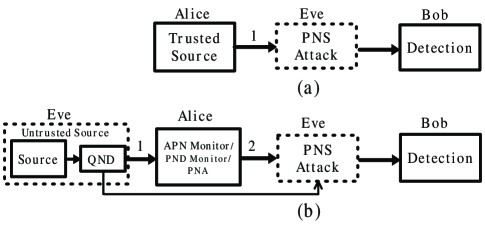
Figure 1: (a) Scheme of “trusted source”. (b) Scheme of “untrusted source”.

However, it was recently found that the characteristics of the QKD source need to be verified in a real-life experiment Gisin et al. (2006); Wang et al. (2007); Wang (2007); Wang et al. (2008, 2009); Zhao et al. (2008); Peng et al. (2008); Moroder et al. (2009); Curty et al. (2009); Adachi et al. (2009); Xu et al. (2009). For example, the intensity fluctuation from the source makes the assumption of the trusted source fail in decoy-state protocol, for which a rigorous security analysis has been given Wang et al. (2007, 2008, 2009). Especially, the assumption of a trusted source does not hold in the round-way “Plug & Play” system Stucki et al. (2002), in which Bob sends to Alice a train of bright laser pulses which can be eavesdropped and controlled by Eve. Even though Alice can use a time (frequency) -domain filter and phase randomizer Zhao et al. (2007) to assure the mixture of single-mode Fork states Gisin et al. (2006); Zhao et al. (2008); Peng et al. (2008), the PND of classically mixed states is under Eve’s control provided that Eve has the power of a quantum nondemolition (QND) measurement Walls and Milburn (1994) and then she can know the photon number of each pulse sent to Alice’s station. This kind of source is defined as an “untrusted source” [see Fig. 1(b)]. Note that Alice’s filters, phase randomizer and encoder exist in Alice’s side which are not shown in Fig. 1(b). Through QND in Fig. 1(b), Eve knows the exact photon number at position 1, which may assist her PNS attack at position 2 Zhao et al. (2008).

For applying the BB84 protocol in the experiment, an average photon number (APN) monitor for an untrusted source was proposed Stucki et al. (2002). However, until now no quantitative and/or detailed analysis to prove the effectiveness of the method was reported. For keeping the efficient decoy-state analysis for an untrusted source, it was proposed to estimate the lower and upper bounds of a few parameters about the PND at position 2 in Fig. 1(b) Wang et al. (2007, 2008, 2009). Recently, the detector-decoy scheme was theoretically proposed to monitor the PND of untrusted source using a threshold detector Moroder et al. (2009). From another viewpoint, an active scheme of the photon number analyzer (PNA) is put forward Zhao et al. (2008) even though it is hard to put into reality Peng et al. (2008). In a recent work, a passive scheme of PNA was proposed and experimentally tested though some practical issues (e.g., statistical fluctuation and detection noise) were not considered Peng et al. (2008).

In the following, the security analysis is made for the APN monitor and the PNA. For the PNA, some practical issues, such as statistical fluctuation due to a finite number of measurements (estimated by the Clopper-Pearson confidence interval Clopper and Pearson (1934); Larsen and Marx (1986)) and two kinds of additive detection noise (Poissonian and Gaussian electronic noise) are analyzed. It shows that the PNA has better enhancement in a secure key rate than the APN monitor and so is more applicable in BB84 protocol.

II security analysis for the APN monitor

A passive scheme is illustrated in Fig. 2 where the detector is limited to monitor the APN ($\mu$) of the untrusted source and an attenuator (transmittance: $\lambda$) is used to ensure the weak pulses with the fixed APN (such as 0.1). This simple intensity monitor has been implemented to a practical “Plug & Play” system Stucki et al. (2002). Applying the BB84 protocol without the decoy states, the security analysis of the untrusted source is presented below. For convenience, in the following discussion, P$i$ with $i=1,\ldots$, refers to the position $i$.

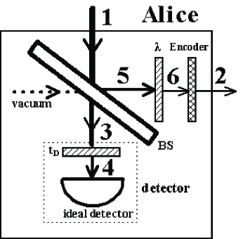
Figure 2: The passive scheme using a beam splitter (BS, transmittance: $t_{B}$), a detector (efficiency: $t_{D}$), an attenuator (transmittance: $\lambda$), and an encoder. Here, the imperfect detector is modeled by a virtual attenuator between P3 and P4 (transmittance: $t_{D}$) and an ideal detector (efficiency: $100\%$). The encoder is used for phase coding.

In Fig. 2, the photoelectron number distribution $D(m)$ at P4 and the PND $P(n_{2})$ at P2 are the Bernoulli transform of PND $P(n_{1})$ at P1, that is

$$D(m) = B[P(n_{1}),\xi]=\sum_{n_{1}=m}^{\infty}P(n_{1}){n_{1}\choose m}\xi^{m}(1-\xi)^{n_{1}-m},$$ (1)

$$P(n_{2}) = B[P(n_{1}),\eta]=\sum_{n_{1}=n_{2}}^{\infty}P(n_{1}){n_{1}\choose n_{2}}\eta^{n_{2}}(1-\eta)^{n_{1}-n_{2}},$$ (2)

where $\eta=\lambda(1-t_{B})$ and $\xi=t_{B}t_{D}$. In practice, the intensity monitor of the detector only gives $\langle m\rangle=\sum_{m=0}^{\infty}mD(m)$. However, based on Eq. (1), $\mu=\langle n_{1}\rangle=\langle m\rangle/\xi$ is known if $\langle m\rangle$ and $\xi$ are both exactly known. Then, from Eq. (2), the APN $\langle n_{2}\rangle$ ($=\eta\mu$) at P2 can be derived. From the work of GLLP, BLMS: see authors of Refs. Gottesman et al. (2004); Brassard et al. (2000), Alice should estimate the upper (lower) bound of multiphoton (single-photon) probability at P2. For the untrusted source only under Alice’s APN monitor, Eve can arbitrarily manipulate $P(n_{1})$ with the constrains of $\sum_{n_{1}=0}^{\infty}n_{1}P(n_{1})=\mu$ and $\sum_{n_{1}=0}^{\infty}P(n_{1})=1$. Eve chooses the optimal $P(n_{1})$ to maximize the multiphoton probability at P2 for eavesdropping more information by the PNS attack. Alice has to estimate the worst case and the upper bound of the multiphoton probability is estimated at P2, which is

$$P(n_{2}>1) =\sum_{n_{1}=2}^{\infty}P(n_{1}){n_{1}\choose 2}\eta^{2}(1-\eta)^{n_{1}-2}+\cdots$$ (3)

$$=a_{2}P(n_{1}=2)+\cdots+a_{k}P(n_{1}=k)+\cdots,$$

where $a_{k}=1-(1-\eta)^{k}-k\eta(1-\eta)^{k-1}~{}(k\geq 2)$. Thus, to estimate the worst case, one needs to solve the convex optimization Boyd and Vandenberghe (2004) or linear program (LP) problem which has the form

$$\rm{minimize}{} -c^{T}x,$$ (4)

$$\rm{subject~{}to}{} Ax=b,~{}x\geq 0,$$

where

$$x=\left[\begin{array}[]{llllll}P(n_{1}=0)&P(n_{1}=1)&P(n_{1}=2)&\cdots&P(n_{1}=k)&\cdots\end{array}\right]^{T},$$ (6)

$$c^{T}=\left[\begin{array}[]{llllll}0&0&a_{2}&\cdots&a_{k},&\cdots\end{array}\right],$$ (8)

$$A=\left[\begin{array}[]{llllcl}0&1&2&\cdots&k&\cdots\\ 1&1&1&\cdots&1&\cdots\\ \end{array}\right],$$

$$b=\left[\begin{array}[]{l}\mu\\ 1\\ \end{array}\right].$$ (12)

The LP problem can be solved by using the simplex method Press et al. (1986) and the maximum value $\overline{P}_{n_{2}>1}$ of $c^{T}x$ is given as

$$\overline{P}_{n_{2}>1}=\frac{a_{k_{s}}\mu}{k_{s}},$$ (13)

where $a_{k_{s}}/k_{s}$ is the maximum value of $a_{k}/k$, and the optimal $P(n_{1})$ of the untrusted source for Eve has the form $\left[P(n_{1}=0)=1-\mu/k_{s},P(n_{1}=k_{s})=\mu/k_{s},P(n_{1}\neq 0,k_{s})=0\right]$. For example, if $\eta=0.001$ and $\mu=100$ are fixed, the simplex method gives that $\overline{P}_{n_{2}>1}=0.02985$ when $P(n_{1}=0)=1-\mu/1794$, $P(n_{1}=1794)=\mu/1794$, and $P(n_{1}\neq 0,1794)=0$.

For an error-free setup with Bob’s perfect detection ($100\%$ detection efficiency and no dark counts), the necessary condition for security is Brassard et al. (2000)

$$\overline{\Delta}=\frac{\overline{P}_{n_{2}>1}}{Q_{e}}<1,$$ (14)

where $Q_{e}$ is the total expected probability of detection events and $\overline{\Delta}$ is the upper bound of tagged signal probability Gottesman et al. (2004). Otherwise, Eve can suppress the single-photon signals completely and obtain full information on the multiphoton signals. In the “Plug & Play” system, the expected photon source entering Alice’s side is Poissonian with APN $\mu$ (i.e., $Q_{e}=1-e^{-\mu\eta\eta_{f}}$). Here, $\eta_{f}=10^{-\alpha^{\prime}L/10}$ is the transmittance of communication fiber with the loss $\alpha^{\prime}$ (0.21 dB/km@1550 nm) and the length $L$. With $\mu=100,~{}\eta=0.001,~{}\alpha^{\prime}=0.21$, and $\overline{P}_{n_{2}>1}=0.02985$, by Eq. (14), the secure transmission distance $L<24.7$ km. Note that, in the same setup, if Alice successfully monitors the PND of the untrusted source at P1 or P2 and Eve does not replace the Poissonian source, the secure transmission distance $L<63$ km. Generally, for a practical “Plug & Play” setup with quantum bit error rate (QBER) $E_{e}$, the secure key rate for an untrusted source with the APN monitor is

$$R\geq\frac{1}{2}Q_{e}\left\{-f\left(E_{e}\right)H_{2}(E_{e})+(1-\overline{\Delta})\left[1-H_{2}\left(\frac{E_{e}}{1-\overline{\Delta}}\right)\right]\right\},$$ (15)

where $f(E_{e})H_{2}(E_{e})$ is the leakage information in the error correction and $H_{2}(x)=-x\log_{2}x-(1-x)\log_{2}(1-x)$. From the above analysis, one cannot find the secure key rate through 67 km fiber in Stucki et al. (2002).

The APN monitor does not require high detector resolution. In the experiment, an optical power meter records the time average of the total pulse energy during one fixed period and is commonly used to monitor the mean optical power or APN $\langle m\rangle$. Due to finite average time, the measured values of the power meter may statistically fluctuate between different periods. Thus, one of the records from the power meter cannot represent the real $\langle m\rangle$ unless it has an infinite average time. However, when the running time of the QKD system is much longer than the average time of the power meter and the large number of records from the power meter are obtained, approximately, the mean of these records obeys the normal distribution according to the central limit theorem (CLT) Papoulis and Pillai (2001). Through the mean and variance of these records, the real $\langle m\rangle$ can be statistically estimated in an interval $[\langle m\rangle^{L},\langle m\rangle^{U}]$ with a confidence level Papoulis and Pillai (2001). Further, with the same confidence level, $\mu\in[\mu^{L},\mu^{U}]$ can be estimated, where $\mu^{L}=\langle m\rangle^{L}/\xi$ and $\mu^{U}=\langle m\rangle^{U}/\xi$. From Eq. (13), $\overline{P}_{n_{2}>1}$ can be estimated by $a_{k_{s}}\mu^{U}/k_{s}$.

III security analysis for the PNA

The passive setup in Fig. 2 can realize the PNA which leads to different analysis results Zhao et al. (2008). By replacing the parameter $\lambda$ and randomly choosing the vacuum state and the signal (weak decoy) state with $\lambda_{s}$ ($\lambda_{d}$), the three-intensity decoy-state protocol can be applied Peng et al. (2008).

The PNA needs to estimate the lower bound of the fraction $1-\delta$ of the photon pulses (defined as “untagged bits” and are originally referred to as P1 in Fig. 2 Zhao et al. (2008)), and the photon number $N$ of which falls in the preset range of $[N_{\rm{min}},N_{\rm{max}}]$. To estimate $1-\delta$, a detector needs to monitor the PND at P4, which is used to yield that at P1 using the inverse-Bernoulli transform Peng et al. (2008). Another important parameter to estimate the secure key rate is the transmittance $\lambda^{A}$ for “untagged bits” in Alice’s side [for those at P1, $\lambda^{A}=(1-t_{B})\lambda$].

The effectiveness of inverse-Bernoulli-transform algorithm is sensitive to the statistical fluctuation and the detection noise, and high-resolution detection is required. To implement the passive scheme more robustly, the detection mode at P4 needs to be simplified, and the effects of statistical fluctuation and the detection noise need to be included in the security analysis. In doing so, a two-threshold detection illustrated in Fig. 3 is used and the position of “untagged bits” is redefined. In Fig. 3, through an integrator, the voltage $v$ denotes the photon number $m$ which is detected by a common photodiode. Two comparators would output “11” when $v\in[v_{1},v_{2}]$, which means the photon number $m$ at P4 falls in $[m_{1},m_{2}]$ where $m_{1}$ and $m_{2}$ correspond to $v_{1}$ and $v_{2}$, respectively.

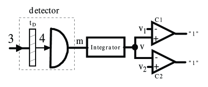
Figure 3: A two-threshold detection for the PNA. The integrator converts the photoelectron number $m$ to the voltage $v$. C1 (C2): comparator. “11” output from C1 and C2 means the voltage $v$ between $v_{1}$ and $v_{2}$ and the photon number $m$ falls in the range $[m_{1},m_{2}]$, correspondingly.

To discuss the position and transmittance of “untagged bits” in the passive scheme of a two-threshold detection mode, we consider three cases according to different parameters of the beam splitter (BS), attenuator, and detector in Fig. 2.

Case I $\left(t_{B}t_{D}=1-t_{B}\right)$:

The “untagged bits” are redefined as the photon pulses with photon number $n_{5}\in[m_{1},m_{2}]$ at P5 in Fig. 2. Thus, the lower probability bound of $1-\delta$ $\left(=\sum_{n_{5}=m_{1}}^{m_{2}}P(n_{5})\right)$ of the “untagged bits” needs to be estimated. Note that $t_{B}t_{D}=1-t_{B}$, $P(n_{5})$ ($=B[P(n_{1}),(1-t_{B})]$) at P5 is equal to $D(m)$ ($=B[P(n_{1}),t_{B}t_{D}]$) at P4 in Fig. 2. Thus, $1-\delta$ is estimated by $\sum_{m=m_{1}}^{m_{2}}D(m)$ and $\lambda^{A}=\lambda$.

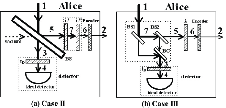
Figure 4: The virtual passive schemes equivalent to Fig. 2 for Cases II and III. (a) Both $\lambda^{\prime}$ $\left(=t_{B}t_{D}/(1-t_{B})\right)$ and $\lambda^{\prime\prime}$ $(=\lambda/\lambda^{\prime})$ are the cascaded attenuators which replace $\lambda$ of Fig. 2. (b) BS1: beam splitter (transmittance, $1-t_{B}t_{D}$); BS2: beam splitter (transmittance, $(1-t_{B})/(t_{B}t_{D})$); BC: beam combiner. BS1, BS2 and BC replace the BS of Fig. 2.

Case II $\left(\lambda\leq t_{B}t_{D}/(1-t_{B})<1\right)$:

The attenuator $\lambda$ in Fig. 2 is virtually replaced by two cascaded attenuators $\lambda^{\prime}$ $\left[=t_{B}t_{D}/(1-t_{B})\right]$ and $\lambda^{\prime\prime}$ $(=\lambda/\lambda^{\prime})$, in which the security is not reduced. A virtual passive scheme [Fig. 4(a)] is equivalent to that of Fig. 2 because the PND at P1 is the same as that at P2, P3, P4, P5 and P6 in both passive schemes. Note that $\lambda^{\prime\prime}\leq 1$ requires $\lambda\leq t_{B}t_{D}/(1-t_{B})$ for the BB84 protocol and $\lambda_{d}<\lambda_{s}\leq t_{B}t_{D}/(1-t_{B})$ for the decoy-state protocol. In Fig. 4(a), the “untagged bits” are defined as the photon pulses with photon number $n_{7}\in[m_{1},m_{2}]$ at P7. Thus, the lower probability bound of $1-\delta$ $\left(=\sum_{n_{7}=m_{1}}^{m_{2}}P(n_{7})\right)$ of “untagged bits” needs to be estimated. Note that $t_{B}t_{D}=(1-t_{B})\lambda^{\prime}$, $P(n_{7})$ at P7 is equal to $D(m)$ at P4 in Fig. 4(a). Thus, $1-\delta$ is estimated by $\sum_{m=m_{1}}^{m_{2}}D(m)$ and $\lambda^{A}=\lambda^{\prime\prime}=(1-t_{B})\lambda/(t_{B}t_{D})$.

Case III ($t_{B}t_{D}>1-t_{B}$):

The BS in Fig. 2 is virtually replaced by two beam splitters (BS1 and BS2) and a beam combiner (BC) [Fig. 4(b)] because the PND at P1 is the same as that at P2, P3, P4, P5 and P6 in both passive schemes. In Fig. 4(b), the “untagged bits” are defined as the photon pulses with photon number $n_{7}\in[m_{1},m_{2}]$ at P7. Note that $P(n_{7})$ at P7 is equal to $D(m)$ at P4 in Fig. 4(b). Thus, the lower probability bound of $1-\delta$ $\left(=\sum_{n_{7}=m_{1}}^{m_{2}}P(n_{7})\right)$ of the “untagged bits” is estimated by $\sum_{m=m_{1}}^{m_{2}}D(m)$ and $\lambda^{A}=(1-t_{B})\lambda/(t_{B}t_{D})$.

The general form of $\lambda^{A}$ for the above cases is thus $(1-t_{B})\lambda/(t_{B}t_{D})$, which is also derived in Zhao et al. (2009). Note that, in our method, the lower bound of $\sum_{m=m_{1}}^{m_{2}}D(m)$ should be estimated by the measured data from the detection mode shown in Fig. 3.

III.1 PNA without detection noise

Let the random variable $R=1$ denote that C1 and C2 output “11”, otherwise $R=0$. Thus, $R$ follows the binomial distribution $B\left(1,p\right)$. Without any detection noise in Fig. 3, $p=\sum_{m=m_{1}}^{m_{2}}D(m)=1-\delta$. After $M$ repeating measurements, let the random variable $X=k$ denote $k$ measurements finding $R=1$ and then $X$ follows the binomial distribution $B\left(M,p\right)$. Statistically, $k/M$ fluctuates around $p$. To estimate the statistical fluctuation, we give the following Lemma.

Lemma. (Clopper-Pearson Confidence Interval Clopper and Pearson (1934); Larsen and Marx (1986)) Let $X$ be the number of successes in $M$ Bernoulli trials with probability $p$ of success on each trial. The Clopper-Pearson ($1-\alpha$) confidence interval for $p$ is obtained as follows: If $X=x$ is observed, then the lower and upper bounds $p_{l}(x,\alpha)$ and $p_{u}(x,\alpha)$, respectively, are defined by

$$\sum_{j=x}^{M}{M\choose j}p_{l}^{j}(x,\alpha)\left[1-p_{l}(x,\alpha)\right]^{M-j}=\frac{\alpha}{2},~{}(1\leq x\leq M);$$

$$\sum_{j=0}^{x}{M\choose j}p_{u}^{j}(x,\alpha)\left[1-p_{u}(x,\alpha)\right]^{M-j}=\frac{\alpha}{2},~{}(0\leq x\leq M-1);$$

$$p_{l}(0,\alpha)=0,~{}p_{u}(M,\alpha)=1.$$ (16)

Obviously, from the Lemma, one has

$${\rm{Prob}}(p_{l}(k,\alpha)\leq p\leq p_{u}(k,\alpha))=1-\alpha.$$ (17)

Thus, $1-\delta$ or $p$ can be lower bounded by $p_{l}(k,\alpha)$ with a confidence level $1-\alpha$, while $p_{l}(k,\alpha)$ can be easily calculated using the MATLAB program.

III.2 PNA with known and additive detection noise

In practice, some detection noise exists in Fig. 3 and affects the estimation of $1-\delta$. Here, it is supposed that the properties of detection noise are known by Alice and are independent of signal detection. Two kinds of noise are mainly concerned. One is Poissonian noise or dark counts from the detector itself. The other is Gaussian electronic noise generated by electronic devices such as the integrator and comparators in Fig. 3. Let the random variables $m^{\prime}$, $m$ and $d$ (or $x$) be measured data, true photon number, and additive Poissonian noise (Gaussian electronic noise) and satisfy

$$m^{\prime}=m+d,~{}m^{\prime}=m+x.$$ (18)

For the Poissonian noise $d$ of the probability $N(d)=\exp(-\gamma)\gamma^{d}/d!$, based on Eq. (18), one yields

$$P(m_{1}\leq m^{\prime}\leq m_{2})= \sum_{m=0}^{m_{1}-1}D(m)\sum_{d=m_{1}-m}^{m_{2}-m}N(d)$$ (19)

$$+\sum_{m=m_{1}}^{m_{2}}D(m)\sum_{d=0}^{m_{2}-m}N(d).$$

Let

$$\overline{b}(m_{1},m_{2}) =\max\left\{\sum_{d=m_{1}-m}^{m_{2}-m}N(d),m=0,\ldots,m_{1}-1\right\},$$ (20)

$$b(m_{2}) =\sum_{d=0}^{m_{2}}N(d).$$

Note that $b(m_{2})\geq\overline{b}(m_{1},m_{2})$. Combining Eqs. (19) and (20), one has

$$P(m_{1}\leq m^{\prime}\leq m_{2})\leq\overline{b}(m_{1},m_{2})\sum_{m=0}^{m_{1}-1}D(m)+b(m_{2})\sum_{m=m_{1}}^{m_{2}}D(m)$$

$$\leq\overline{b}(m_{1},m_{2})\left[\sum_{m=0}^{m_{1}-1}D(m)+\sum_{m=m_{2}+1}^{\infty}D(m)\right]+b(m_{2})\sum_{m=m_{1}}^{m_{2}}D(m)$$

$$=\overline{b}(m_{1},m_{2})\left[1-\sum_{m=m_{1}}^{m_{2}}D(m)\right]+b(m_{2})\sum_{m=m_{1}}^{m_{2}}D(m),$$ (21)

which gives

$$1-\delta=\sum_{m=m_{1}}^{m_{2}}D(m)\geq\frac{P(m_{1}\leq m^{\prime}\leq m_{2})-\overline{b}(m_{1},m_{2})}{b(m_{2})-\overline{b}(m_{1},m_{2})}.$$ (22)

After $M$ measurements of $m^{\prime}$, if one finds $k^{\prime}$ events from the binomial distribution $B(M,p^{\prime})$, according to the Lemma,

$${\rm{Prob}}(p_{l}(k^{\prime},\alpha)\leq p^{\prime}\leq p_{u}(k^{\prime},\alpha))=1-\alpha,$$ (23)

where $p^{\prime}=P(m_{1}\leq m^{\prime}\leq m_{2})$. From Eqs. (22) and (23), $1-\delta$ can be lower bounded by

$$1-\delta\geq\frac{p_{l}(k^{\prime},\alpha)-\overline{b}(m_{1},m_{2})}{b(m_{2})-\overline{b}(m_{1},m_{2})}$$ (24)

with a confidence level $1-\alpha$.

For the case of electronic noise $x$ of the Gaussian probability $G(x)=(2\pi\sigma^{2})^{-1/2}\exp\big{[}-x^{2}/(2\sigma^{2})\big{]}$, based on Eq. (18), one yields

$$P(m_{1}\leq m^{\prime}\leq m_{2})=\sum_{m=0}^{m_{1}-1}D(m)\int_{m_{1}-m}^{m_{2}-m}G(x)dx$$

$$+\sum_{m=m_{1}}^{m_{2}}D(m)\int_{m_{1}-m}^{m_{2}-m}G(x)dx+\sum_{m=m_{2}+1}^{\infty}D(m)\int_{m_{1}-m}^{m_{2}-m}G(x)dx$$

$$\leq\sum_{m=0}^{m_{1}-1}D(m)\int_{0}^{m_{2}-m_{1}}G(x)dx+\sum_{m=m_{1}}^{m_{2}}D(m)\int_{-(m_{2}-m_{1})/2}^{(m_{2}-m_{1})/2}G(x)dx$$

$$+\sum_{m=m_{2}+1}^{\infty}D(m)\int_{m_{1}-m_{2}-1}^{-1}G(x)dx.$$ (25)

To derive the above inequality, the property that $G(x)$ is single-peak function symmetrical at zero is used. Let

$$b_{1} =\int_{0}^{m_{2}-m_{1}}G(x)dx,~{}b_{2}=\int_{-(m_{2}-m_{1})/2}^{(m_{2}-m_{1})/2}G(x)dx,$$ (26)

$$b_{3} =\int_{m_{1}-m_{2}-1}^{-1}G(x)dx,$$

and $b_{2}\geq b_{1}\geq b_{3}$. Equation (III.2) then changes to

$$P(m_{1}\leq m^{\prime}\leq m_{2})$$ (27)

$$\leq b_{1}\left[\sum_{m=0}^{m_{1}-1}D(m)\right]+b_{2}\left[\sum_{m=m_{1}}^{m_{2}}D(m)\right]+b_{3}\left[\sum_{m=m_{2}+1}^{\infty}D(m)\right]$$

$$\leq b_{1}\left[\sum_{m=0}^{m_{1}-1}D(m)+\sum_{m=m_{2}+1}^{\infty}D(m)\right]+b_{2}\left[\sum_{m=m_{1}}^{m_{2}}D(m)\right]$$

$$=b_{1}\left[1-\sum_{m=m_{1}}^{m_{2}}D(m)\right]+b_{2}\left[\sum_{m=m_{1}}^{m_{2}}D(m)\right].$$

Thus, we get

$$1-\delta=\sum_{m=m_{1}}^{m_{2}}D(m)\geq\frac{P(m_{1}\leq m^{\prime}\leq m_{2})-b_{1}}{b_{2}-b_{1}}.$$ (28)

Similar to Eq. (24), $1-\delta$ can be lower bounded by

$$1-\delta\geq\frac{p_{l}(k^{\prime},\alpha)-b_{1}}{b_{2}-b_{1}}$$ (29)

with a confidence level $1-\alpha$.

IV Numerical Simulations

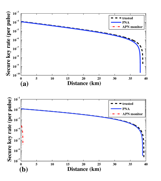
Figure 5: (Color online) The simulations of the BB84 protocol for the trusted source and untrusted source with the APN monitor and PNA. (a) $\eta=(\eta_{B}\eta_{f})/\mu$ and parameters in Gobby et al. (2004) are used. (b) $\eta=10^{-7}$, $\eta_{B}=0.5$ and other parameters are the same as Gobby et al. (2004).

Based on the BB84 protocol, Fig. 5 shows the numerical simulation results for a trusted source and an untrusted source with an APN monitor and PNA. In the simulations, both the trusted and untrusted sources are of Poissonian PND. The APN ($\mu$) of the untrusted source is $10^{6}$. We use the passive scheme of $t_{B}=0.9$ and $t_{D}=0.76$ to implement the APN monitor and PNA without considering statistical fluctuation and detection noise. Figure 5(a) shows the result with the experimental parameters in Gobby et al. (2004) (see Table 1), where $\eta_{B}$ is the efficiency of Bob’s detection, $Y_{0}$ is the dark-count rate of Bob’s detector, and $e_{\rm{det}}$ ($e_{0}$) is the probability that a photon (dark count) hit the erroneous detector in Bob’s side. In Fig. 5(a), we choose the optimized value of $\eta=(\eta_{B}\eta_{f})/\mu$ for both the trusted and untrusted sources, $f(E_{e})=1$ for perfect error correction and $[m_{1},m_{2}]=[677160,690840]$ for the detection thresholds in Fig. 3. $Q_{e}$ and $E_{e}$ are given by Ma et al. (2005)

$$Q_{e} =Y_{0}+1-\exp(-\mu\eta\eta_{B}\eta_{f}),$$ (30)

$$E_{e} =\frac{e_{0}Y_{0}+e_{\rm{det}}[1-\exp(-\mu\eta\eta_{B}\eta_{f})]}{Q_{e}}.$$

Note that, from Fig. 5(a), no secure key rate with an APN monitor is generated at any distance, while the secure key rate with PNA is found close to the value of the trusted source.

Table 1: The simulation parameters for Fig. 5(a).

$\mu$	$t_{B}$	$t_{D}$	$\eta_{B}$	$\alpha^{\prime}$	$Y_{0}$	$e_{\rm{det}}$	$e_{0}$
$10^{6}$	0.9	0.76	0.045	0.21	$1.7\times 10^{-6}$	3.3%	0.5

For comparing the APN monitor with PNA more visibly and fairly, Fig. 5(b) shows the result with fixing $\eta=10^{-7}$ and resetting $\eta_{B}=0.5$. Other simulation parameters are the same as those in Table 1. Using these parameters, one can fix $\overline{P}_{n_{2}>1}=0.029843$ to calculate the secure key rate with the APN monitor. From Fig. 5(b), the secure distance is shown to be less than 1 km with the APN monitor. Fortunately, PNA improves the performance which approaches that of the trusted source.

For testing the effects of statistical fluctuation and detection noise on PNA, we choose an untrusted source of Poissonian statistics to perform the simulations based on the three-intensity decoy-state protocol. In the passive scheme as in Fig. 2, $t_{B}$ and $t_{D}$ are chosen as 0.9 and 0.76, respectively. The APN of the untrusted source is $1.462\times 10^{7}$. Thus, $\langle m\rangle$ at P4 is $10^{7}$. For applying the decoy-state protocol, the average photon number for a signal (weak decoy) state is $\nu_{s}=0.5$ ($\nu_{d}=0.1$). In doing so, the transmittance of the attenuator is $\lambda_{s}=3.42\times 10^{-7}$ ($\lambda_{d}=6.84\times 10^{-8}$) for the signal (weak decoy) state. The photoelectron detection and additive detection noise generated in Fig. 3 are simulated using the Monte Carlo method and $M=10^{8}$ of measurements are run. Other parameters are chosen from Gobby et al. (2004) and summarized in Table 2.

Table 2: The simulation parameters for Fig. 6.

$\nu_{s}$	$\nu_{d}$	$t_{B}$	$t_{D}$	$\langle m\rangle$	$M$	$\lambda_{s}$	$\lambda_{d}$	$\eta_{B}$	$\alpha^{\prime}$	$Y_{0}$	$e_{\rm{det}}$	$e_{0}$
0.5	0.1	0.9	0.76	$10^{7}$	$10^{8}$	$3.42\times 10^{-7}$	$6.84\times 10^{-8}$	0.045	0.21	$1.7\times 10^{-6}$	3.3%	0.5

With different Poissonian noise ($\gamma=10^{6},\ldots,7\times 10^{6}$) added in the PNA, each color line in Fig. 6(a) shows the secure key rate for the untrusted source. For comparison, the black dashed line shows the secure key rate for the trusted source with the same setup. Here, the confidence level $1-\alpha$ is chosen as $1-10^{-6}$ and the minimal (maximal) value of detected $m^{\prime}$ is chosen as $m_{1}$ ($m_{2}$), by which $p_{l}(M,\alpha)=(\alpha/2)^{1/M}$ can be substituted to Eq. (24) according to the Lemma.

With different Gaussian electronic noise ($\sigma^{2}=10^{9},\ldots,7\times 10^{10}$) added in PNA, each color line in Fig. 6(b) shows the secure key rate for untrusted source. The method of choosing $\alpha,~{}m_{1}$, and $m_{2}$ is the same as that of Poissonian noise.

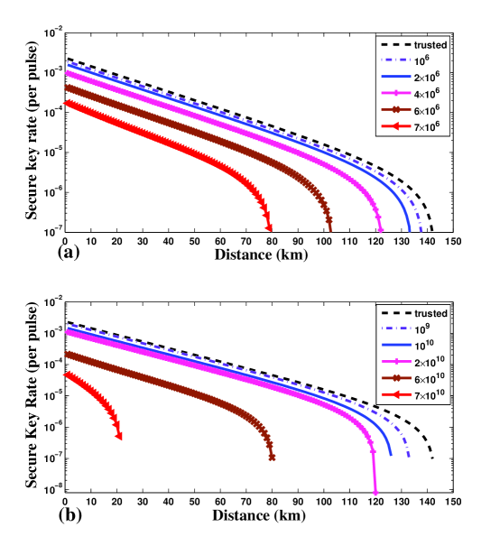
Figure 6: (Color online) The simulations of three-intensity decoy-state protocol for a trusted source and untrusted source with PNA with different detection noise, run by $M=10^{8}$ and $\alpha=10^{-6}$. (a) Poissonian noise with the average photon number $\gamma=10^{6},\ldots,7\times 10^{6}$. (b) Gaussian electronic noise with variance $\sigma^{2}=10^{9},\ldots,7\times 10^{10}$.

V Conclusion

In the passive scheme as in Fig. 2, a different monitor mode at P4 gives different statistical characteristics of the untrusted source and affects the performance of the QKD system. It is shown from Fig. 5 that the PNA can enhance the QKD performance better than the APN monitor because PNA utilizes the two-threshold detection as in Fig. 3. Asymptotically, if the photon statistics at P1 can be fully characterized through a photon-number-resolving (PNR) detector at P3 and the PND monitor can be realized, the GLLP’s analysis for the trusted source can be efficiently applied and the results are shown as the black dashed line in Figs. 5 and 6. Without considering the statistical fluctuation and detection noise, the secure key rate through PNA approaches that of an ideal PND monitor except at a long distance. What is more important is that the two-threshold detection mode of PNA is easier to realize than the PNR detector. Besides, it is also found from Fig. 6 that too large a random noise added in the PNA’s detection would degenerate the QKD performance. Thus, for improving the secure key rate, the signal-to-noise ratio (SNR) in Fig. 3 needs to be kept in an applicable level. For example, in our simulations, $R^{SN}_{p}=\langle m\rangle/\gamma$ and $R^{SN}_{g}=\langle m\rangle/\sigma^{2}$ can be calculated for Poissonian and Gaussian electronic noise, respectively. From Fig. 6, if the QKD distance would exceed 120 km, then $R^{SN}_{p}\geq 2.5$ and $R^{SN}_{g}\geq 5\times 10^{-4}$ are needed and is achievable in practice. Therefore, the passive scheme with PNA is highly practical to solve the untrusted source problem in the “Plug & Play” QKD system.

We remark that the effect of parameter fluctuations has not yet been included in the security analysis. The effective method to deal with the parameter fluctuations Wang et al. (2007); Wang (2007); Wang et al. (2008, 2009) is encouraged to be applied in the passive scheme.

Note added. For passive scheme, the security analysis with considering statistical fluctuation and detection noise for PNA is given with using different techniques Zhao et al. (2009).

References

- Bennett and Brassard (1984) C. H. Bennett and G. Brassard, in Proceedings of IEEE International Conference on Computers, Systems, and Signal Processing (IEEE, New York, 1984).
- Ekert (1991) A. K. Ekert, Phys. Rev. Lett. 67, 661 (1991).
- Gisin et al. (2002) N. Gisin, G. Ribordy, W. Tittel, and H. Zbinden, Rev. Mod. Phys. 74, 145 (2002).
- Dušek et al. (2006) M. Dušek, N. Lütkenhaus, and M. Hendrych, Prog. in Opt. 49, 381 (2006).
- Lo and Zhao (2008) H. K. Lo and Y. Zhao, arXiv: quant-ph/0803.2507 (2008).
- Scarani et al. (2009) V. Scarani, H. Bechmann-Pasquinucci, N. J. Cerf, M. Dušek, N. Lütkenhaus, and M. Peev, Rev. Mod. Phys. 81, 1301 (2009).
- Lo and Chau (1999) H. K. Lo and H. F. Chau, Science 283, 2050 (1999).
- Shor and Preskill (2000) P. W. Shor and J. Preskill, Phys. Rev. Lett. 85, 441 (2000).
- Mayers (2001) D. Mayers, J. ACM 48, 351 (2001).
- Inamori et al. (2007) H. Inamori, N. Lütkenhaus, and D. Mayers, Eur. Phys. J. D 41, 599 (2007).
- Gottesman et al. (2004) D. Gottesman, H. K. Lo, N. Lütkenhaus, and J. Preskill, Quant. Inf. Comput. 4, 325 (2004).
- Lütkenhaus (2000) N. Lütkenhaus, Phys. Rev. A 61, 052304 (2000).
- Brassard et al. (2000) G. Brassard, N. Lütkenhaus, T. Mor, and B. C. Sanders, Phys. Rev. Lett. 85, 1330 (2000).
- Lütkenhaus and Jahma (2002) N. Lütkenhaus and M. Jahma, New J. Phys. 4, 44 (2002).
- Hwang (2003) W. Y. Hwang, Phys. Rev. Lett. 91, 057901 (2003).
- Wang (2005a) X. B. Wang, Phys. Rev. Lett. 94, 230503 (2005a).
- Lo et al. (2005) H. K. Lo, X. Ma, and K. Chen, Phys. Rev. Lett. 94, 230504 (2005).
- Wang (2005b) X. B. Wang, Phys. Rev. A 72, 012322 (2005b).
- Ma et al. (2005) X. Ma, B. Qi, Y. Zhao, and H. K. Lo, Phys. Rev. A 72, 012326 (2005).
- Rosenberg et al. (2007) D. Rosenberg, J. W. Harrington, P. R. Rice, P. A. Hiskett, C. G. Peterson, R. J. Hughes, A. E. Lita, S. W. Nam, and J. E. Nordholt, Phys. Rev. Lett. 98, 010503 (2007).
- Schmitt-Manderbach et al. (2007) T. Schmitt-Manderbach, H. Weier, M. Fürst, R. Ursin, F. Tiefenbacher, T. Scheidl, J. Perdigues, Z. Sodnik, C. Kurtsiefer, J. G. Rarity, et al., Phys. Rev. Lett. 98, 010504 (2007).
- Peng et al. (2007) C. Z. Peng, J. Zhang, D. Yang, W.-B. Gao, H. X. Ma, H. Yin, H. P. Zeng, T. Yang, X. B. Wang, and J. W. Pan, Phys. Rev. Lett. 98, 010505 (2007).
- Yuan et al. (2007) Z. L. Yuan, A. W. Sharpe, and A. J. Shields, Appl. Phys. Lett. 90, 011118 (2007).
- Gisin et al. (2006) N. Gisin, S. Fasel, B. Kraus, H. Zbinden, and G. Ribordy, Phys. Rev. A 73, 022320 (2006).
- Wang et al. (2007) X. B. Wang, T. Hiroshima, A. Tomita, and M. Hayashi, Phys. Rep. 448, 1 (2007).
- Wang (2007) X. B. Wang, Phys. Rev. A 75, 052301 (2007).
- Wang et al. (2008) X. B. Wang, C. Z. Peng, J. Zhang, L. Yang, and J. W. Pan, Phys. Rev. A 77, 042311 (2008).
- Wang et al. (2009) X. B. Wang, L. Yang, C. Z. Peng, and J. W. Pan, New J. Phys. 11, 075006 (2009).
- Zhao et al. (2008) Y. Zhao, B. Qi, and H. K. Lo, Phys. Rev. A 77, 052327 (2008).
- Peng et al. (2008) X. Peng, H. Jiang, B. J. Xu, X. Ma, and H. Guo, Opt. Lett. 33, 2077 (2008).
- Moroder et al. (2009) T. Moroder, M. Curty, and N. Lütkenhaus, New J. Phys. 11, 045008 (2009).
- Curty et al. (2009) M. Curty, T. Moroder, X. Ma, and N. Lütkenhaus, Opt. Lett. 34, 3238 (2009).
- Adachi et al. (2009) Y. Adachi, T. Yamamoto, M. Koashi, and N. Imoto, New J. Phys. 11, 113033 (2009).
- Xu et al. (2009) F. X. Xu, Y. Zhang, Z. Zhou, W. Chen, Z. F. Han, and G. C. Guo, Phys. Rev. A 80, 062309 (2009).
- Stucki et al. (2002) D. Stucki, N. Gisin, O. Guinnard, G. Ribordy, and H. Zbinden, New J. Phys. 4, 41 (2002).
- Zhao et al. (2007) Y. Zhao, B. Qi, and H. K. Lo, Appl. Phys. Lett. 90, 044106 (2007).
- Walls and Milburn (1994) D. F. Walls and G. J. Milburn, Quantum Optics (Springer-Verlag, Berlin, Heidelberg, 1994).
- Clopper and Pearson (1934) C. J. Clopper and E. S. Pearson, Biometrika 26, 404 (1934).
- Larsen and Marx (1986) R. J. Larsen and M. L. Marx, An Introduction to Mathematical Statistics and Its Applications (Prentice-Hall, NewJersey, 1986), p 279.
- Boyd and Vandenberghe (2004) S. Boyd and L. Vandenberghe, Convex Optimization (Cambridge University Press, Cambridge, 2004).
- Press et al. (1986) W. H. Press, B. P. Flannery, S. A. Teukolsky, and W. T. Vetterling, Numerical Recipes (Cambridge University Press, Cambridge, 1986).
- Papoulis and Pillai (2001) A. Papoulis and S. U. Pillai, Probability, Random Variables and Stochastic Processes (McGraw-Hill, New York, 2002).
- Zhao et al. (2009) Y. Zhao, B. Qi, H. K. Lo, and L. Qian, arXiv: quant-ph/0905.4225 (2009).
- Gobby et al. (2004) C. Gobby, Z. L. Yuan, and A. J. Shields, Appl. Phys. Lett. 84, 3762 (2004).