Interfacial instability of turbulent two-phase stratified flow: Multi-equation turbulent modelling with rapid distortion

Abstract

We investigate the linear stability of a flat interface that separates a liquid layer from a fully-developed turbulent gas flow. In this context, linear-stability analysis involves the study of the dynamics of a small-amplitude wave on the interface, and we develop a model that describes wave-induced perturbation turbulent stresses (PTS). We demonstrate the effect of the PTS on the stability properties of the system in two cases: for a laminar thin film, and for deep-water waves. In the first case, we find that the PTS have little effect on the growth rate of the waves, although they do affect the structure of the perturbation velocities. In the second case, the PTS enhance the maximum growth rate, although the overall shape of the dispersion curve is unchanged. Again, the PTS modify the structure of the velocity field, especially at longer wavelengths. Finally, we demonstrate a kind of parameter tuning that enables the production of the thin-film (slow) waves in a deep-water setting.

I Introduction

Understanding the stability of a flat interface separating the liquid and gas phases in a turbulent boundary layer is a long-standing problem OceanwavesBook . In this paper, we focus in detail on one aspect of this problem, namely modelling the perturbation turbulent stresses that arise when a wave on the interface interacts with the turbulence and generates Reynolds stresses. The approach we take has multiple facets: we derive a model velocity field describing the base turbulent flow in the system, and we then perform a linear-stability analysis around this base state using the Orr–Sommerfeld formalism. We construct a detailed model to describe the turbulent stresses that appear in these linear-stability equations. Motivated by the paper of Ierley and Miles Miles2001 , we use a model that linearly couples the streamfunction to the turbulent kinetic energy and Reynolds stresses, and divides the gas domain into near-equilibrium and rapid-distortion regions.

The purpose of our investigation is twofold. In the present paper, we develop a model that describes in detail the averaged effects of turbulence on the linear stability of the gas-liquid interface. We carry out some preliminary calculations for two archetypal cases: the thin liquid film sheared by a turbulent gas flow, and the generation of interfacial waves over deep water. This model forms the basis for a more detailed study of the thin-film case (in a pressure-driven scenario), which is reported elsewhere Onaraigh2_2009 . Since the present work focusses on turbulent gas-liquid instability in general, we place our work in context by describing the studies that have been performed on similar gas-liquid systems in the past.

The generation of waves by wind:

The problem of computing the growth rate of an interfacial instability for a turbulent gas-liquid system was first considered by Jeffreys Jeffreys1925 , Phillips Phillips1957 , and Miles Miles1957 . Phillips studied a resonant interaction between turbulent pressure fluctuations and capillary-gravity waves on an interface, while Miles focussed on a particular kind of shear inviscid flow that produces linear instability. In the paper of Miles, in later works by the same author Miles1959 ; Miles1962b , and in the work of Benjamin Benjamin1958 , the liquid layer is neglected, and is replaced by a wavy wall, and the problem is reduced to computing the stress exerted on the interface by the turbulent gas flow. Energy transfer from the gas to the interface is governed by the second derivative of the mean flow. Indeed, the growth rate of the instability is determined by the sign of the second derivative of the mean flow at the critical height – the height at which the mean flow and wave speed are equal. Recent work of Lin et al. lin2008 indicates that the Phillips mechanism may be important in an initial regime, leading to wave growth that is approximately linear in time. Their results show that this is followed by an exponential growth regime, which is primarily governed by the disturbances in the flow induced by the waves themselves. In this paper, we focus on this latter stage; we shall investigate the effects of the presence of short waves (possibly induced by a Phillips-type mechanism) on this exponential wave growth regime in a later, more detailed, study.

Modelling Reynolds stresses:

In these early works Miles1957 ; Miles1959 ; Miles1962b ; Benjamin1958 , the turbulent nature of the gas flow is taken into account through the prescription of a logarithmic mean profile in the gas. Nevertheless, the Reynolds stress terms that enter into the stability equations are ignored. This problem is rectified by Van Duin and Janssen Janssen1992 , and by Belcher and co-workers in a series of papers Belcher1993 ; Belcher1994 ; Belcher1998 . The latter group studies the interfacial stability of a sheared air-water interface, and specialize to an air-water system for oceanographical applications. With the exception of Belcher1994 , they treat the interface in a manner similar to Miles. Particular care is taken in developing an understanding of the structure of the turbulent shear stresses inherent in the problem through the use of scaling arguments and a truncated mixing-length model. This is representative of an approximation of a Reynolds-averaged ensemble of realizations of the turbulent flow for a given phase of a small-amplitude interfacial wave. In this approach, an eddy viscosity is formulated in terms of the typical scale of a turbulent eddy, which depends on the distance between the eddy itself and the air-water interface. Far from the interface, the turbulent eddies are advected quickly over an interfacial undulation, and have insufficient time to equilibrate, and so-called rapid-distortion theory is needed. Such an approach was developed by Townsend Townsend1979 . In the papers of Belcher and co-workers, however, the far-field region is simply modelled by the Rayleigh equation. Thus, the mixing-length is truncated: it is a simple function of the vertical co-ordinate close to the interface, and is set to zero far from the interface. We propose instead to follow the approach of Townsend Townsend1979 and Ierley and Miles Miles2001 : not only do we interpolate between the turbulent domains (a common factor between all these papers), but we also explicitly model the rapid-distortion region. Our model is based on the linearized closure model of the Reynolds-averaged equations pioneered by Launder et al. LRR1975 and discussed in the book by Pope TurbulencePope .

Numerical approaches:

The work discussed so far uses asymptotic techniques for the determination of stability. Numerical methods provide more information on the stability, since they are valid over all parameter ranges, and since they readily enable the re-construction of the velocity and pressure fields from the solution of an eigenvalue problem. The paper of Boomkamp and Miesen Boomkamp1996 provides yet more information, since they classify interfacial instabilities according to an energy budget: the contributions to the time-change in kinetic energy are derived from the linearized Navier–Stokes equations, and several destabilizing factors are identified. Of interest in the present application are the critical-layer mechanism and the viscosity-contrast mechanism. In this approach Miesen1995 ; Boomkamp1996 , and in similar work by Özgen Ozgen1998 ; Ozgen2008 , the viscous liquid layer and gas layers are modelled co-equally; these added complications necessitate a numerical solution of the equation. The interfacial wave speed is then determined, along with the growth rate, as the solution of an eigenvalue problem. Turbulence enters the problem only though the logarithmic mean-flow profile chosen, and the Reynolds stress terms are ignored.

Modelling of the base flow:

The papers mentioned so far use a model of the base flow that captures its logarithmic shape. These base models contain a free parameter, however, since the interfacial friction velocity $U_{*\mathrm{i}}$ is undetermined. In the approach we take, we use a closed model that fixes this parameter as a function of the Reynolds number. Our formalism is based on that introduced by Biberg Biberg2007 , although it differs in one key respect: we pay close attention to the near-interface modelling (and also to the modelling near the upper wall, if present), and remove the singularities that arise when the logarithm in the velocity is evaluated an upper wall or an interface. This is accomplished using a Van Driest interpolation TurbulencePope ; demekhin2006 , in which the velocity field smoothly transitions between the log layer and the viscous near-wall (interfacial) region.

These are the ingredients of our model, which we develop in the following way. In Sec. II we provide a detailed description of the rapid-distortion and near-equilibrium turbulence which we constitute in terms of the streamfunction. We introduce the Orr–Sommerfeld equation for the streamfunction, which couples to the turbulent stresses. In Sec. III we describe the numerical method used to solve the model equations. In Sec. IV we describe the effects of the turbulent modelling on a thin-film flow (this problem was studied in the absence of perturbation turbulent stresses by Miesen and Boersma Miesen1995 ). We find that the growth rate is not significantly affected by the turbulence modelling, although the structure of the flow field is. Nevertheless, for deep-water waves (Sec. V), both the growth rate and the flow structure are modified by the turbulence (the growth rate is enhanced). In this deep-water study, we compare our results with direct numerical simulation, and investigate a mechanism for generating thin-film type waves in a deep water setting. Finally, in Sec. VI we present our conclusions.

II Theoretical formulation

In this section we provide a problem description and develop a turbulence model that takes account of rapid distortion and near-equilibrium regions in the turbulent stratified two-phase flow. Our approach is inspired by the paper of Miles Miles2001 . It takes into account the interactions between interfacial waves and the turbulence. The work here is, however, multi-faceted: there is a model of the flat-interface turbulent state, together with a linear-stability analysis around this state, in which the effects of the turbulence are modelled in detail. The two-layer system we consider has the same structure as boundary-layer flow, and is described schematically in Fig. 1. A rectangular co-ordinate system is used to model the flow, with the plane $z=0$ coinciding with the undisturbed location of the interface. Since the interfacial waves that develop are two-dimensional, we restrict to a two-dimensional system, in which the bottom layer is a liquid of depth $d_{L}$, which in this paper will either be a thin laminar layer, or a deep-water flow ($d_{L}=\infty$). The top layer is gaseous, turbulent and fully-developed. A shear stress

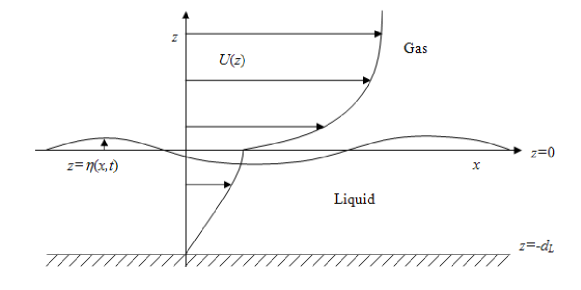
Figure 1: A schematic diagram showing the system of interest. There is turbulent shear flow in the gas layer, while the liquid layer either represents a thin laminar film, or deep-water flow, as in oceans.

is applied along the channel. The mean profile is thus a uni-directional flow in the horizontal, $x$-direction. In the gas layer, near the gas-liquid interface and the gas-wall boundary, the flow is dominated by molecular viscosity, since here the viscous scale exceeds the characteristic length scale of the turbulence TurbulenceMonin ; TurbulencePope . In the bulk of the gas region, the flow possesses a logarithmic profile TurbulenceMonin ; TurbulencePope . Finally, we assume that the gas-liquid interface is smooth.

II.1 The perturbation equations

Following standard practice dating back to Miles Miles1957 , we base the dynamical equations for the interfacial motion on the Reynolds-averaged Navier–Stokes (RANS) equations. The turbulent velocity is decomposed into averaged and fluctuating parts $\bm{U}=\left(U,W\right)$ and $\left(u^{\prime},w^{\prime}\right)$ respectively. The averaged velocity depends on space and time through the RANS equations:

$$\rho\left(\frac{\partial U_{i}}{\partial t}+\bm{U}\cdot\nabla U_{i}\right)=-\frac{\partial P}{\partial x_{i}}+\mu\Delta U_{i}-\rho\left(\frac{\partial}{\partial x}\langle u^{\prime}u_{i}^{\prime}\rangle+\frac{\partial}{\partial z}\langle w^{\prime}u_{i}^{\prime}\rangle\right),\qquad i=x,z,$$ (1a)

$$\nabla\cdot\bm{U}=0,$$ (1b)

where $\langle\cdot\rangle$ denotes the averaging process. The constants $\rho$ and $\mu$ denote the density and viscosity respectively. In addition to viscous stress, Eq. (1a) contains a stress term that arises due to the interaction between the turbulence and the mean flow. We use these equations to model a flat-interface or base state of the two-phase system shown in Fig. 1. Next, we introduce a small disturbance that shifts the flat interface at $z=0$ to $z=\eta$, where $|\eta|\ll 1$, and this induces a change in the average velocity and pressure fields, denoted as follows:

$$\left(U,W,P\right)=\left(U_{0}\left(z\right)+\delta u\left(x,z,t\right),\delta w\left(x,z,t\right),P_{0}\left(x,z\right)+\delta p\left(x,z,t\right)\right),$$

where we denote base-state quantities by a subscript zero. Since the flow is turbulent, and since the perturbations take the form of waves, they must satisfy the RANS equations for a linear wave of speed $c$, $\partial_{t}=-c\partial_{x}$:

$$\rho\left[\left(U_{0}-c\right)\frac{\partial}{\partial x}\delta u+\frac{\mathrm{d}{U_{0}}}{\mathrm{d}{z}}\delta{w}\right]=-\frac{\partial}{\partial x}\left(\delta p-\rho\delta\sigma_{z}\right)+\mu\left(\frac{\partial^{2}}{\partial x^{2}}+\frac{\partial^{2}}{\partial z^{2}}\right)\delta u+\rho\frac{\partial}{\partial x}\delta\sigma+\rho\frac{\partial}{\partial z}\delta\tau,$$ (2a)

$$\rho\left(U_{0}-c\right)\frac{\partial}{\partial x}\delta w=-\frac{\partial}{\partial z}\left(\delta p-\rho\delta\sigma_{z}\right)+\mu\left(\frac{\partial^{2}}{\partial x^{2}}+\frac{\partial^{2}}{\partial z^{2}}\right)\delta w+\rho\frac{\partial}{\partial x}\delta\tau,$$ (2b)

$$\frac{\partial}{\partial x}\delta u+\frac{\partial}{\partial z}\delta w=0.$$ (2c)

The quantities

$$\delta\tau=-\langle u^{\prime}w^{\prime}\rangle-\tau^{(0)},\,\,\delta\sigma_{x}=-\langle u^{\prime 2}\rangle-\sigma_{x}^{(0)},\,\,\delta\sigma_{z}=-\langle w^{\prime 2}\rangle-\sigma_{z}^{(0)},\,\,\delta\sigma=\delta\sigma_{x}-\delta\sigma_{z}$$

are the perturbation stresses due to the turbulence in the perturbed state, while the quantities with the zero-superscript are base-state stresses. Using the streamfunction representation $\left(\delta u,\delta w\right)=\left(\phi_{z},-\phi_{x}\right)$, and the normal-mode decomposition $\partial_{x}=i\alpha$, the perturbed RANS equations reduce to a single equation:

$$i\alpha\rho\left[\left(U_{0}-c\right)\mathrm{D}^{2}\phi-\frac{\mathrm{d}^{2}U_{0}}{\mathrm{d}z^{2}}\phi\right]=\mu\left(\mathrm{D}^{2}-\alpha^{2}\right)^{2}\phi+\rho i\alpha\mathrm{D}\delta\sigma+\left(\mathrm{D}^{2}+\alpha^{2}\right)\delta\tau,$$ (3)

where $\mathrm{D}=\mathrm{d}/\mathrm{d}z$.

II.2 Separation of domains

To model the turbulent stresses in detail, we need to understand the features of the turbulence. Because the instabilities we observe arise due to conditions in the gas, we pay particular attention to the gas layer. If the liquid layer is deep, then the standard Orr–Sommerfeld equation gives an appropriate description of the flow there, provided an accurate base-state profile is supplied Boomkamp1996 ; Zeisel2007 , while if the liquid resides in a thin layer, the Orr–Sommerfeld equation gives an exact description of the flow. Thus, in both cases, we specify the standard Orr–Sommerfeld equation in the liquid, without the additional stresses. The turbulence in the gas is characterised by two timescales: the eddy turnover timescale, and the advection timescale. Roughly speaking, the eddy turnover or turbulent timescale is the time required for a typical turbulent eddy to interact with the surrounding fluid and come into equilibrium (where the production equals dissipation). An estimate of this timescale, at a distance $z$ from the interface, is $T_{\mathrm{t}}=\kappa z/U_{*\mathrm{i}}$, where $\kappa$ is the Von Kármán constant, $\kappa=0.41$, and $U_{*\mathrm{i}}$ is the friction velocity at the interface. The advection timescale is the time needed for the flow to advect an eddy over a wave crest. This flow distorts the turbulence and moves it away from equilibrium. An estimate of this timescale is $T_{\mathrm{a}}=\left[\alpha\left|U_{0}\left(z\right)-c\right|\right]^{-1}$, where $\alpha$ is the wavenumber and $c$ is the complex the wave speed. These eddy-turnover and advection effects compete: near the interface, $T_{\mathrm{t}}$ is small compared with $T_{\mathrm{a}}$, that is, the frequency of turbulent interactions is large compared with the frequency of advection events. This is the region of near-equilibrium where by definition eddy viscosity and one-equation turbulent closures are expected to be appropriate. Far away from the interface, $T_{\mathrm{t}}$ is large compared with the advection timescale (at least for the large, most energetic turbulent structures), or equivalently, the frequency of turbulent interactions is small compared with the frequency of advection events. This is the region where rapid-distortion theory is expected to apply Belcher1993 ; Belcher1994 ; Belcher1998 . In an obvious way, we call the region where eddy viscosity and one-equation formalisms are appropriate the near-interface region, while the region where the rapid-distortion calculations work is called the far-field region. Crossover occurs at $z=z_{\mathrm{t}}$, for which $T_{\mathrm{t}}\left(z_{\mathrm{t}}\right)=T_{\mathrm{a}}\left(z_{\mathrm{t}}\right)$. For further discussion of this separation of domains, see Cohen1998 ; Belcher1998 .

II.3 Turbulence modelling in the distinct domains

In modelling the perturbation turbulent stresses (PTS), we are particularly interested in the anisotropy tensor

$$\mathsf{n}_{ij}=\frac{\langle u^{\prime}_{i}u^{\prime}_{j}\rangle}{\langle u^{\prime}_{k}u^{\prime}_{k}\rangle}=\frac{\mathsf{r}_{ij}}{q}=-\left(\begin{array}[]{cc}\frac{\sigma_{x}}{q}&\frac{\tau}{q}\\ \frac{\tau}{q}&\frac{\sigma_{z}}{q}\end{array}\right),$$ (4)

where $q=2k=\mathrm{tr}\left(\mathsf{r}_{ij}\right)$, and $k$ is the turbulent kinetic energy. The exact equations for the fluctuating component of the velocity in the RANS equations are

$$\left(\frac{\partial}{\partial t}+\bm{U}\cdot\nabla\right)u^{\prime}_{i}=\frac{\partial\mathsf{r}_{ik}}{\partial x_{k}}-u^{\prime}_{k}\frac{\partial U_{i}}{\partial x_{k}}-u_{k}^{\prime}\frac{\partial u_{i}^{\prime}}{\partial x_{k}}+\nu\nabla^{2}u_{i}^{\prime}-\frac{1}{\rho}\frac{\partial p^{\prime}}{\partial x_{i}},\qquad\nu=\frac{\mu}{\rho}.$$ (5)

In the far field, the mean strain produced by the wave is large. We therefore study the equations of motion in the limit of strong mean strain. In that case the terms involving gradients of fluctuating quantities drop out:

$$\left(\frac{\partial}{\partial t}+\bm{U}\cdot\nabla\right)u^{\prime}_{i}=-u^{\prime}_{k}\frac{\partial U_{i}}{\partial x_{k}}-\frac{1}{\rho}\frac{\partial p^{(r)}}{\partial x_{i}},$$ (6)

where

$$\frac{1}{\rho}\nabla^{2}p^{(r)}=-2\frac{\partial U_{i}}{\partial x_{j}}\frac{\partial u^{\prime}_{j}}{\partial x_{i}},$$

with $p^{(r)}$ being the so-called rapid pressure. By a straightforward manipulation of Eq. (6),

$$\frac{\partial\mathsf{r}_{ij}}{\partial t}+\frac{\partial}{\partial x_{k}}\left(U_{k}\mathsf{r}_{ij}+\mathcal{T}_{kij}\right)=\mathcal{P}_{ij}+\mathcal{R}_{ij}^{(r)},$$ (7)

in the limit of strong mean strain, where the tensor quantities have the following meaning:

• The production of stress by the mean flow:

  $$\mathcal{P}_{ij}=-\mathsf{r}_{ik}\frac{\partial U_{j}}{\partial x_{k}}-\mathsf{r}_{jk}\frac{\partial U_{i}}{\partial x_{k}};$$

• The transport of stress by the rapid pressure:

  $$\mathcal{T}_{kij}=-\frac{1}{\rho}\langle u^{\prime}_{i}p^{(r)}\rangle\delta_{jk}-\frac{1}{\rho}\langle u^{\prime}_{j}p^{(r)}\rangle\delta_{ik}$$

• The pressure rate-of-strain term:

  $$\mathcal{R}_{ij}^{(r)}=\bigg{\langle}\frac{p^{(r)}}{\rho}\left(\frac{\partial u^{\prime}_{i}}{\partial x_{j}}+\frac{\partial u^{\prime}_{j}}{\partial x_{i}}\right)\bigg{\rangle}$$

For waves, the shear rate $\alpha\left(U_{0}-c\right)$ enters into the advection term in Eq. (7). In the rapid-distortion domain, this rate is large, and thus advective transport dominates over pressure-driven transport. We therefore omit the pressure transport term in (7), which now simplifies further:

$$\left(\frac{\partial}{\partial t}+\bm{U}\cdot\nabla\right)\mathsf{r}_{ij}=\mathcal{P}_{ij}+\mathcal{R}_{ij}^{(r)},$$ (8)

Equation (8) contains only one term that is not available in closed form: the rapid pressure-rate of strain tensor $\mathcal{R}_{ij}^{(r)}$. This term has been modelled accurately by Launder, Reece and Rodi LRR1975 (see also TurbulencePope ). They use the following form:

$$\mathcal{R}_{ij}^{(\mathrm{r})}=-C_{\mathrm{I}}\left(\mathcal{P}_{ij}-\tfrac{1}{2}\mathcal{P}_{kk}\delta_{ij}\right),$$ (9)

where $C_{\mathrm{I}}=\tfrac{3}{5}$. This model also has the property of linearity in the tensor $\mathsf{r}_{ij}$, which is desirable in any rapid-distortion theory TurbulencePope . The advection equation (8) now becomes

$$\frac{\partial\mathsf{r}_{ij}}{\partial t}+\bm{U}\cdot\nabla\mathsf{r}_{ij}=\left(1-C_{\mathrm{I}}\right)\mathcal{P}_{ij}+\tfrac{1}{2}C_{\mathrm{I}}\mathcal{P}_{kk}\delta_{ij}.$$ (10)

Using the definition (4) and Eq. (10), the $\mathsf{n}_{ij}$’s satisfy the relation

$$\frac{\partial\mathsf{n}_{ij}}{\partial t}+\bm{U}\cdot\nabla\mathsf{n}_{ij}=-\left(1-C_{\mathrm{I}}\right)\mathsf{n}_{ik}\frac{\partial U_{j}}{\partial x_{k}}-\left(1-C_{\mathrm{I}}\right)\mathsf{n}_{jk}\frac{\partial U_{i}}{\partial x_{k}}-2\mathsf{n}_{k\ell}\frac{\partial U_{\ell}}{\partial x_{k}}\left(\tfrac{1}{2}C_{\mathrm{I}}\delta_{ij}-\mathsf{n}_{ij}\right).$$

We decompose the tensor $\mathsf{n}_{ij}$ into a flat-interface component and a perturbation component: $\mathsf{n}_{ij}=\mathsf{n}_{ij}^{(0)}+\delta\mathsf{n}_{ij}$, where $\mathsf{n}_{ij}^{(0)}$ is the equilibrium anisotropy tensor, and is thus constant in time. Hence,

$$\mathsf{n}_{12} = \mathsf{n}_{12}^{(0)}-\frac{1}{q_{0}}\left(\delta\tau+\mathsf{n}_{12}^{(0)}\delta q\right),$$

$$\mathsf{n}_{11} = \mathsf{n}_{11}^{(0)}-\frac{1}{q_{0}}\left(\delta\sigma_{x}+\mathsf{n}_{11}^{(0)}\delta q\right),$$

$$\mathsf{n}_{22} = \mathsf{n}_{22}^{(0)}-\frac{1}{q_{0}}\left(\delta\sigma_{z}+\mathsf{n}_{22}^{(0)}\delta q\right),$$

where $q_{0}\left(z\right)$ represents twice the turbulent kinetic energy associated with the base state and $\delta q$ a small-amplitude perturbation about this state. We therefore have perturbation equations for $\delta\mathsf{n}_{12}$ and $\delta\mathsf{n}:=\delta\mathsf{n}_{11}-\delta\mathsf{n}_{22}$:

$$\left(\frac{\partial}{\partial t}+\bm{U}\cdot\nabla\right)\delta\mathsf{n}_{12} = \alpha_{1}\frac{\partial}{\partial z}\delta{u}+\alpha_{2}\frac{\partial}{\partial{x}}\delta{w}+\alpha_{3}\frac{\partial}{\partial{x}}\delta{u}+\alpha_{4}\delta\mathsf{n}_{12}+\alpha_{5}\delta\mathsf{n},$$

$$\left(\frac{\partial}{\partial t}+\bm{U}\cdot\nabla\right)\delta\mathsf{n} = \beta_{1}\frac{\partial}{\partial z}\delta{u}+\beta_{2}\frac{\partial}{\partial{x}}\delta{w}+\beta_{3}\frac{\partial}{\partial{x}}\delta{u}+\beta_{4}\delta\mathsf{n}_{12}+\beta_{5}\delta\mathsf{n}.$$ (11)

Given the base-state shear rate $\Sigma=\mathrm{d}U_{0}/\mathrm{d}z$, the coefficients in Eqs. (11) are defined as follows:

$$\alpha_{1} = 2\left(\mathsf{n}^{(0)}_{12}\right)^{2}-\left(1-C_{\mathrm{I}}\right)\mathsf{n}^{(0)}_{11},$$

$$\alpha_{2} = 2\left(\mathsf{n}^{(0)}_{12}\right)^{2}-\left(1-C_{\mathrm{I}}\right)\mathsf{n}^{(0)}_{22},$$

$$\alpha_{3} = 2\mathsf{n}^{(0)}_{12}\left(\mathsf{n}^{(0)}_{11}-\mathsf{n}^{(0)}_{22}\right),$$

$$\alpha_{4} = 4\Sigma\mathsf{n}^{(0)}_{12},$$

$$\alpha_{5} = \tfrac{1}{2}\Sigma\left(1-C_{\mathrm{I}}\right),$$

$$\beta_{1} = 2\mathsf{n}^{(0)}_{12}\left(\mathsf{n}^{(0)}_{11}-\mathsf{n}^{(0)}_{22}\right)-2\left(1-C_{\mathrm{I}}\right)\mathsf{n}^{(0)}_{12},$$

$$\beta_{2} = 2\mathsf{n}^{(0)}_{12}\left(\mathsf{n}^{(0)}_{11}-\mathsf{n}^{(0)}_{22}\right)+2\left(1-C_{\mathrm{I}}\right)\mathsf{n}^{(0)}_{12},$$

$$\beta_{3} = 2\left(\mathsf{n}^{(0)}_{11}-\mathsf{n}^{(0)}_{22}\right)^{2}-2\left(1-C_{\mathrm{I}}\right)\left(\mathsf{n}^{(0)}_{11}+\mathsf{n}^{(0)}_{22}\right),$$

$$\beta_{4} = 2\Sigma\mathsf{n}^{(0)}_{12},$$

$$\beta_{5} = 2\Sigma\left[\left(\mathsf{n}^{(0)}_{11}-\mathsf{n}^{(0)}_{22}\right)-2\left(1-C_{\mathrm{I}}\right)\right].$$

Far from the interface, the effects of rapid distortion due to the base flow are negligible, since the shear rate $\Sigma\left(z\right)$ is small there; thus $\alpha_{4}$, $\alpha_{5}$, $\beta_{4}$, and $\beta_{5}$ are small and are neglected in this formalism. In Secs. IV and V, we estimate the $\mathsf{n}_{ij}^{(0)}$’s by constant values obtained from the properties of log layer in turbulent shear flow. Then, Eq. (11), in normal-mode form, reduces to a set of equations that are algebraic in $\delta\mathsf{n}_{12}$ and $\delta\mathsf{n}$:

$$i\alpha\left(U_{0}-c\right)\delta\mathsf{n}_{12} = \alpha_{1}\frac{\partial}{\partial z}\delta{u}+\alpha_{2}\frac{\partial}{\partial{x}}\delta{w}+\alpha_{3}\frac{\partial}{\partial{x}}\delta{u},$$

$$i\alpha\left(U_{0}-c\right)\delta\mathsf{n} = \beta_{1}\frac{\partial}{\partial z}\delta{u}+\beta_{2}\frac{\partial}{\partial{x}}\delta{w}+\beta_{3}\frac{\partial}{\partial{x}}\delta{u}.$$ (12)

The right-hand side of both these equations can easily be recast in terms of the streamfunction, using $\left(\partial/\partial z\right)\delta u=\mathrm{D}^{2}\phi$ etc. However, to highlight the effect of the distortion of the Reynolds stresses by the perturbation velocity, we leave Eq. (12) in its present form throughout the paper.

The derivation of a near-field model is less involved. Near the interface, the turbulence tends quickly to equilibrium, and the $\mathsf{n}_{ij}$’s take their constant value. Thus,

$$\delta\mathsf{n}_{ij}=0.$$ (13)

Next, we develop a strategy to join up these domains and the models (11) and (13) into a single formalism. This requires a detailed picture of the turbulent kinetic energy.

II.4 Turbulent kinetic energy

The governing equation for the perturbation turbulent kinetic energy $\delta k=\tfrac{1}{2}\langle u^{\prime 2}+w^{\prime 2}\rangle-k_{0}$ can be written as:

$$\frac{\partial}{\partial t}\delta k+\bm{U}_{0}\cdot\nabla\delta k+\delta\bm{U}\cdot\nabla k=-\nabla\cdot\left(\delta\bm{J}\right)+\delta\mathcal{P}-\delta\varepsilon,$$

where the terms are explained in detail in what follows. Using the properties of the basic state, this equation reduces to

$$\frac{\partial}{\partial t}\delta k+U_{0}\frac{\partial}{\partial x}\delta k+\delta w\frac{\mathrm{d}k_{0}}{\mathrm{d}z}=-\nabla\cdot\left(\delta\bm{J}\right)+\delta\mathcal{P}-\delta\varepsilon.$$

We now turn to the problem of modelling the terms on the right-hand side of this equation.

• The energy flux: In Townsend Townsend1972 ; Townsend1979 and Ierley and Miles Miles2001 , the energy flux $\delta\bm{J}$ is ignored, since turbulent transport is negligible in the bulk gas flow. It is important, however, near the interface, where molecular viscosity dominates. We therefore take $\delta\bm{J}=-\nu\nabla\delta k$.

• Dissipation: In previous works, Townsend1972 ; Townsend1979 ; Miles2001 , the dissipation function $\delta\varepsilon$ in the bulk gas region was constructed as a cumbersome function of $k_{0}$ and the mixing length. In this work, we make use of the simple model

  $$\delta\varepsilon=\frac{1}{\chi}\delta k,$$

  where $\chi$ is a timescale constructed from dimensional analysis:

  $$\chi=\frac{\nu}{U_{*\mathrm{i}}^{2}},$$

  We have verified that the choice of form for this relation makes little difference to the results of the stability calculation, and we therefore settle on the linear form, which has the added advantage that $\chi^{-1}$ does not diverge at $z=0$.

• Production: The production of turbulent kinetic energy is half the trace of $\mathcal{P}_{ij}$, and thus the perturbed production rate has the form

  $$\delta\mathcal{P}=-\delta\mathsf{r}_{ij}\frac{\partial U_{i}^{(0)}}{\partial x_{j}}-\mathsf{r}_{ij}^{(0)}\frac{\partial}{\partial x_{j}}\delta U_{i},$$

  which can be re-expressed as

  $$\delta\mathcal{P}=\delta\tau\frac{\mathrm{d}U_{0}}{\mathrm{d}z}+\tau^{(0)}\left(\mathrm{D}^{2}+\alpha^{2}\right)\phi+i\alpha\mathrm{D}\phi\left(\sigma_{x}^{(0)}-\sigma_{z}^{(0)}\right),$$

  where $\delta\tau=-\langle u^{\prime}w^{\prime}\rangle-\tau^{(0)}$ is the perturbed turbulent shear stress, and $\tau^{(0)}$, $\sigma_{x}^{(0)}$, and $\sigma_{z}^{(0)}$ represent the turbulent stresses in the flat-interface state. Thus, we obtain the following kinetic-energy equation:

  $$i\alpha\left(U_{0}-c\right)\delta k+\chi^{-1}\delta k\\ =\nu\left(\mathrm{D}^{2}-\alpha^{2}\right)\delta k-\delta\mathsf{r}_{12}\frac{\mathrm{d}U_{0}}{\mathrm{d}z}-\mathsf{r}_{12}^{(0)}\left(\mathrm{D}^{2}+\alpha^{2}\right)\phi-i\alpha\mathsf{r}^{(0)}\mathrm{D}\phi+i\alpha\frac{\mathrm{d}k_{0}}{\mathrm{d}z}\phi,$$

  where $\mathsf{r}^{(0)}=-\left(\sigma_{x}^{(0)}-\sigma_{z}^{(0)}\right)$ and $\mathsf{r}_{12}^{(0)}=-\tau^{(0)}$.

II.5 Interpolation between domains

The algebraic model for the tensor $\delta\mathsf{n}_{ij}$ is given by Eq. (12) in the far field, and by Eq. (13) in the near field. We can interpolate between these domains by using a hybrid stress model:

$$\left[i\alpha\left(U_{0}-c\right)\mathcal{I}\left(z\right)+\left(1-\mathcal{I}\left(z\right)\right)\right]\delta\mathsf{n}_{12}=\mathcal{I}\left(z\right)\left(\alpha_{1}\frac{\partial}{\partial z}\delta{u}+\alpha_{2}\frac{\partial}{\partial{x}}\delta{w}+\alpha_{3}\frac{\partial}{\partial{x}}\delta{u}\right),$$

$$\left[i\alpha\left(U_{0}-c\right)\mathcal{I}\left(z\right)+\left(1-\mathcal{I}\left(z\right)\right)\right]\delta\mathsf{n}=\mathcal{I}\left(z\right)\left(\beta_{1}\frac{\partial}{\partial z}\delta{u}+\beta_{2}\frac{\partial}{\partial{x}}\delta{w}+\beta_{3}\frac{\partial}{\partial{x}}\delta{u}\right),$$

where $\mathcal{I}\left(z\right)$ is an interpolating function that is zero at $z=0$ and asymptotes to $\mathcal{I}=1$, with a characteristic lengthscale $z_{\mathrm{t}}$.

We now have all the components to assemble the model, which we present below in non-dimensional form. We non-dimensionalize on as-yet undefined length and velocity scales $h$ and $V$ respectively, and the gas viscosity, which gives rise to the gas Reynolds number $Re=Vh/\nu_{G}$. In the liquid, a single equation describes the flow, which in non-dimensional form is simply

$$i\alpha r\left[\left(U_{L}-c\right)\left(\mathrm{D}^{2}-\alpha^{2}\right)\phi_{L}-\frac{\mathrm{d}^{2}U_{L}}{\mathrm{d}z^{2}}\phi_{L}\right]=\frac{m}{Re}\left(\mathrm{D}^{2}-\alpha^{2}\right)^{2}\phi_{L},\qquad z\leq 0,$$ (14a)

where the subscripts ‘L’ and ‘G’ denote evaluation in the gas and liquid phases respectively: $$U_{L} U_{G} r=\rho_{L}/\rho_{G} m=\mu_{L}/\mu_{G}$$ and are the base-state velocities in the liquid and gas phases, and and are the density and viscosity ratios. In the turbulent gas, we must solve the following coupled set of equations:

$$i\alpha\left[\left(U_{G}-c\right)\left(\mathrm{D}^{2}-\alpha^{2}\right)\phi_{G}-\frac{\mathrm{d}^{2}U_{G}}{\mathrm{d}z^{2}}\phi_{G}\right]=\frac{1}{Re}\left(\mathrm{D}^{2}-\alpha^{2}\right)^{2}\phi_{G}-i\alpha\mathrm{D}\delta\mathsf{r}-\left(\mathrm{D}^{2}+\alpha^{2}\right)\delta\mathsf{r}_{12},$$ (14b)

$$\left[i\alpha\left(U_{G}-c\right)+\frac{Re_{*}^{2}}{Re}\right]\delta k\\ =\frac{1}{Re}\left(\mathrm{D}^{2}-\alpha^{2}\right)\delta k-\delta\mathsf{r}_{12}\frac{\mathrm{d}U_{G}}{\mathrm{d}z}-\mathsf{r}_{12}^{(0)}\left(\mathrm{D}^{2}+\alpha^{2}\right)\phi_{G}-i\alpha\mathsf{r}^{(0)}\mathrm{D}\phi+i\alpha\frac{\mathrm{d}k_{0}}{\mathrm{d}z}\phi_{G},$$ (14c)

where $$Re_{*}=U_{*\mathrm{i}}h/\nu_{G} U_{*\mathrm{i}}$$, the Reynolds number based on the interfacial friction velocity , and where

$$\left[i\alpha\left(U_{G}-c\right)\mathcal{I}\left(z\right)+\left(1-\mathcal{I}\left(z\right)\right)\right]\delta\mathsf{r}_{12}-\frac{\mathsf{r}_{12}^{(0)}}{q_{0}}\left[i\alpha\left(U_{G}-c\right)\mathcal{I}\left(z\right)+\left(1-\mathcal{I}\left(z\right)\right)\right]\delta{q}\\ =q_{0}\left(z\right)\mathcal{I}\left(z\right)\left(\alpha_{1}\frac{\partial}{\partial z}\delta{u}+\alpha_{2}\frac{\partial}{\partial{x}}\delta{w}+\alpha_{3}\frac{\partial}{\partial{x}}\delta{u}\right),$$ (14d)

$$\left[i\alpha\left(U_{G}-c\right)\mathcal{I}\left(z\right)+\left(1-\mathcal{I}\left(z\right)\right)\right]\delta\mathsf{r}-\frac{\mathsf{r}^{(0)}}{q_{0}}\left[i\alpha\left(U_{G}-c\right)\mathcal{I}\left(z\right)+\left(1-\mathcal{I}\left(z\right)\right)\right]\delta{q}\\ =q_{0}\left(z\right)\mathcal{I}\left(z\right)\left(\beta_{1}\frac{\partial}{\partial z}\delta{u}+\beta_{2}\frac{\partial}{\partial{x}}\delta{w}+\beta_{3}\frac{\partial}{\partial{x}}\delta{u}\right).$$ (14e)

At the wall $z=-d_{L}/h$, we have the no-slip conditions on the streamfunction $\phi_{L}$,

$$\phi_{L}\left(-d_{L}/h\right)=\mathrm{D}\phi_{L}\left(-d_{L}/h\right)=0.$$

The equations are also matched across the undisturbed interface $z=0$, where we have the following conditions:

$$\phi_{L} =\phi_{G},$$ (15a)

$$\mathrm{D}\phi_{L} =\mathrm{D}\phi_{G}+\frac{\phi_{L}}{c-U_{L}}\left(\frac{\mathrm{d}U_{G}}{\mathrm{d}{z}}-\frac{\mathrm{d}U_{L}}{\mathrm{d}{z}}\right),$$ (15b)

$$m\left(\mathrm{D}^{2}+\alpha^{2}\right)\phi_{L} =\left(\mathrm{D}^{2}+\alpha^{2}\right)\phi_{G}+Re\delta\tau_{G},$$ (15c)

$$m\left(\mathrm{D}^{3}\phi_{L}-3\alpha^{2}\mathrm{D}\phi_{L}\right)+\mathrm{i}\alpha rRe\left(c-U_{L}\right)\mathrm{D}\phi_{L}+i\alpha rRe\frac{\mathrm{d}U_{L}}{\mathrm{d}z}\phi_{L}-\frac{\mathrm{i}\alpha rRe}{c-U_{L}}\left(Fr+\alpha^{2}S\right)\phi_{L}\\ =\left(\mathrm{D}^{3}\phi_{G}-3\alpha^{2}\mathrm{D}\phi_{G}\right)+\mathrm{i}\alpha Re\left(c-U_{L}\right)\mathrm{D}\phi_{G}+i\alpha Re\frac{\mathrm{d}U_{G}}{\mathrm{d}z}\phi_{G}+Re\mathrm{D}\delta\tau+i\alpha Re\delta\sigma,$$ (15d)

where we have introduced the inverse Froude and inverse Weber numbers, respectively

$$Fr=\frac{g\left(\rho_{L}-\rho_{G}\right)h}{\rho_{G}V^{2}},\qquad S=\frac{\sigma}{\rho_{G}V^{2}h}.$$ (16)

Here $g$ and $\sigma$ are the gravity and surface tension constants. For clarity, we shall refer to the inverse Froude number as the gravity number, being the ratio of gravitational to inertial forces, likewise we refer to the inverse Weber number as the surface-tension number.

The turbulent kinetic-energy equation is second-order, and therefore requires only two boundary conditions. We apply the conditions $k_{0}+\delta k=0$ on $z=\eta$ and $z=d_{G}/h$, where $d_{G}/h$ is the non-dimensional vertical extent of the gas layer. For boundary-layer flow, $d_{G}=\infty$, while for channel flow $d_{G}$ is finite. Upon linearization these kinetic energy conditions are

$$\delta k=0\qquad\text{at }z=0,\,\,\text{and at }z=d_{G}/h.$$ (17)

Furthermore, if we take

$$\mathcal{I}\left(0\right)=\frac{\mathrm{d}\mathcal{I}\left(0\right)}{\mathrm{d}z}=0,$$

then, by inspection of Eqs. (14d) and (14e), $\delta\mathsf{r}_{12}=\left(\mathsf{r}_{12}/q\right)\delta q=0$ at $z=0$, and similarly for $\delta\mathsf{r}$ and $\mathrm{D}\delta\mathsf{r}$. (The justification for this choice of $\mathcal{I}$ is given at the end of Sec. IV.1.) Consequently, Eqs. (15d) reduce to the standard interfacial equations:

$$\phi_{L} =\phi_{G},$$ (18a)

$$\mathrm{D}\phi_{L} =\mathrm{D}\phi_{G}+\frac{\phi_{L}}{c-U_{L}}\left(\frac{\mathrm{d}U_{G}}{\mathrm{d}{z}}-\frac{\mathrm{d}U_{L}}{\mathrm{d}{z}}\right),$$ (18b)

$$m\left(\mathrm{D}^{2}+\alpha^{2}\right)\phi_{L} =\left(\mathrm{D}^{2}+\alpha^{2}\right)\phi_{G},$$ (18c)

$$m\left(\mathrm{D}^{3}\phi_{L}-3\alpha^{2}\mathrm{D}\phi_{L}\right)+\mathrm{i}\alpha rRe\left(c-U_{L}\right)\mathrm{D}\phi_{L}+i\alpha rRe\frac{\mathrm{d}U_{L}}{\mathrm{d}z}\phi_{L}-\frac{\mathrm{i}\alpha rRe}{c-U_{L}}\left(Fr+\alpha^{2}S_{\mathrm{cap}}\right)\phi_{L}\\ =\left(\mathrm{D}^{3}\phi_{G}-3\alpha^{2}\mathrm{D}\phi_{G}\right)+\mathrm{i}\alpha Re\left(c-U_{L}\right)\mathrm{D}\phi_{G}+i\alpha Re\frac{\mathrm{d}U_{G}}{\mathrm{d}z}\phi_{G}.$$ (18d)

Finally, at the top of the gas domain $z=d_{G}/h$, we have the requirement that the perturbation velocities should vanish:

$$\phi_{G}\left(d_{G}/h\right)=\mathrm{D}\phi_{G}\left(d_{G}/h\right)=0.$$

Thus, we obtain a total of $10$ conditions, which provides sufficient information to close the system of equations $\left(\phi_{L},\phi_{G},\delta k,\delta\mathsf{r}_{12},\delta\mathsf{r}\right)$. No conditions are required on $\delta\mathsf{r}$, and $\delta\mathsf{r}_{12}$, since these variables appear only in an algebraic way in Eqs. (14d) and (14e). We now turn to the numerical solution of this system of equations

III Numerical method

In the liquid and turbulent gas domains, we propose an approximate solution to the Orr–Sommerfeld (OS) equations (14e)

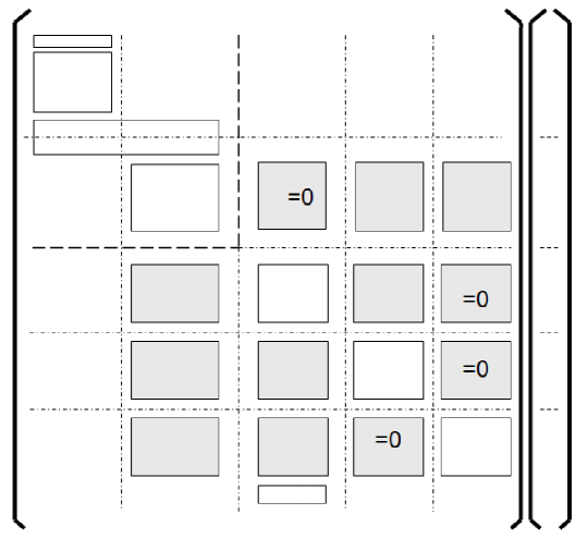
Figure 2: A schematic description of the left-hand side of Eq. (20). The shaded blocks represent the linear interaction between the turbulence variables. The upper right-hand block enclosed by the thick dotted lines is the matrix for the eigenvalue problem in the absence of the turbulent stress and energy variables.

in terms of Chebyshev polynomials, such that

$$\phi_{L}\left(z\right)\approx\sum_{n=0}^{N_{L}}a_{n}T_{n}\left(\eta_{L}\right),\qquad\phi_{G}\left(z\right)\approx\sum_{n=0}^{N_{G}}b_{n}T_{n}\left(\eta_{G}\right),$$ (19a)

$$\delta k=\sum_{n=0}^{N_{G}-2}\zeta_{n}T_{n}\left(\eta_{G,1}\right),\qquad\delta\mathsf{r}_{12}=\sum_{n=0}^{N_{G}-4}\theta_{n}T_{n}\left(\eta_{G}\right),\qquad\delta\mathsf{r}=\sum_{n=0}^{N_{G}-4}\xi_{n}T_{n}\left(\eta_{G}\right),\qquad$$ (19b)

where we have mapped the domains of the various layers into the interval $$[-1,1] z\in\left[-d_{L},0\right] z\in\left[0,d_{G}\right]$$. For our two-layer system, with for the liquid and for the gas turbulent layer, the appropriate coordinate transformations are the following:

$$\eta_{L}=\frac{2z}{d_{L}}+1,\,\,\,-d_{L}\leq z\leq 0 ;\qquad\eta_{G}=\frac{2z}{d_{G}}-1,\,\,0\leq z\leq d_{G}.$$

Thus, we assume that the boundary layer is of finite depth. This setup has the advantage that the gas domain is finite in extent, and thus there are no virtual interfaces in the problem. In our experience, these virtual interfaces can interfere with the stability properties of the system, and are therefore undesirable. Although there are differences between the stability behaviour of the finite- and infinite-domain frameworks, these are apparent only at small $$\alpha$$ (large-wavelength disturbances). We shall also show that this is far from the most dangerous mode, and these differences are therefore unimportant. The derivatives of our approximate solution are obtained through the expressions

$$\frac{\mathrm{d}^{r}\phi_{L}\left(z\right)}{\mathrm{d}z^{r}}=\sum_{n=0}^{N_{L}}a_{n}\left(\frac{\mathrm{d}\eta_{L}}{\mathrm{d}z}\right)^{r}T_{n}^{\left(r\right)}\left(\eta_{L}\right),\qquad\frac{\mathrm{d}^{r}\phi_{G}\left(z\right)}{\mathrm{d}z^{r}}=\sum_{n=0}^{N_{G}}b_{n}\left(\frac{\mathrm{d}\eta_{G}}{\mathrm{d}z}\right)^{r}T_{n}^{\left(r\right)}\left(\eta_{G}\right),$$ (19c)

where the derivatives of the Chebyshev polynomial $T_{n}\left(\eta\right)$ are obtained through the appropriate recurrence relation.

To reduce the problem (14e) to a matrix form, we substitute the approximate solution (19c) into the OS equations (14e) and evaluate the resulting identity at the collocation points

$$\eta_{L} = \cos\left(\frac{p\pi}{N_{L}-2}\right),\qquad p=1,...,N_{L}-3,$$

$$\eta_{G} = \cos\left(\frac{p\pi}{N_{G}-2}\right),\qquad p=1,...,N_{G}-3.$$

In the two-layer application that we have in mind, this gives

$$\left(N_{L}-3\right)+4\left(N_{G,1}-3\right)=N_{L}+4N_{G,1}-15$$

equations in $\left(N_{L}+1\right)+\left(N_{G,1}+1\right)+\left(N_{G,1}-1\right)+2\left(N_{G,1}-3\right)$ $=N_{L}+4N_{G,1}-5$ unknowns. We must therefore find an additional $10$ equations to close the system. These are provided by the $10$ boundary and interfacial conditions. Thus, we are reduced to solving for the wave speed $c$, given $N_{L}+4N_{G,1}-3$ linear equations in as many unknowns. In symbols, we therefore have a generalized eigenvalue problem

$$\mathsf{L}\bm{x}=\lambda\mathsf{M}\bm{x},\qquad\lambda=-i\alpha c,$$ (20)

where positivity of the real part of $\lambda$ ($\lambda_{\mathrm{r}}>0$) indicates instability. A schematic description of the left-hand side of this system is shown in Fig. 2. The solution of (20) is best found using a linear algebra package (as in TrefethenBook ). Then, a built-in eigenvalue solver automatically balances the matrices $\mathsf{L}$ and $\mathsf{M}$, an important issue here since these matrices can be very badly conditioned, owing to the high-order derivatives of the Chebyshev polynomials that appear in the expansion of the streamfunction (as in the work by Boomkamp et al. Boomkamp1997 ). Furthermore, a specialized eigenvalue solver takes into account the appearance of zero rows (hence infinite eigenvalues) in the matrix $\mathsf{M}$, and thus gives an accurate answer. Following standard practice, we modify the number of collocation points until convergence is achieved (typically, $N_{L}=200$, $N_{G}=150$ for convergence to four significant figures).

IV Results for a thin film

In this section, we investigate the effects of turbulence on the interfacial stability of a thin laminar liquid layer exposed to fully-developed turbulent shear flow in an overlying gas layer. The parameter regime we study involves $Re$, $Fr$, $S$, and the ratio

$$\delta=\frac{d_{L}}{d_{G}}=\frac{\text{liquid-film thickness}}{\text{gas-layer thickness}},$$

and is chosen to mimic the conditions in pipe flow in oil-gas transport problems Miesen1995 . The liquid Reynolds number is such that the liquid flow is laminar. We use a base state that mimics flow in a boundary layer. In this case the flow is confined by a flat plat at $z=d_{G}$, a large distance from the interface. This plate moves at velocity $U_{0}$ relative to the interface. It is thus appropriate to re-scale on the velocity $U_{0}$, and on the gas-layer depth $d_{G}$ (thus $h=d_{G}$ and $V=U_{0}$, in the notation of Sec. II). This setup has the advantage that the gas domain is finite in extent, while having little effect on the results (see Fig. 5 for a comparison between finite- and infinite-domain growth rates). Using this framework, we constitute the base-state velocity.

IV.1 Base-state determination

The gas layer:

In the gas, we have the following momentum balance for the base state:

$$\mu_{G}\frac{\mathrm{d}U_{G}}{\mathrm{d}z}+\tau_{TSS}=\tau_{\mathrm{i}},$$ (21a)

where $$\tau_{\mathrm{i}} \tau_{TSS} -\rho_{G}\langle u^{\prime}w^{\prime}\rangle$$ is the interfacial shear stress, and is the turbulent shear stress . To close this term, we make use of the interpolation function

$$G\left(\tilde{z}\right)=\tilde{z}\left(1-\tilde{z}\right),\qquad\tilde{z}=\frac{z}{d_{G}},$$ (21b)

where $$\tilde{z}$$ is the non-dimensional vertical co-ordinate (the tilde decoration has been introduced to designate dimensionless quantities). Now the turbulent shear stress has a characteristic Taylor expansion near the walls, and for the interpolation function (21b) to agree with this expansion, we must modify Eq. (21b) near the upper wall and the interface, such that

$$\tau_{TSS}=\kappa\rho_{G}d_{G}U_{*\mathrm{i}}G\left(\tilde{z}\right)\psi\left(\tilde{z}\right)\psi\left(1-\tilde{z}\right)\frac{\mathrm{d}U_{G}}{\mathrm{d}z},\qquad\psi\left(\tilde{z}\right)=1-e^{-\tilde{z}^{n}/A},$$ (21c)

where $$n A Re U_{*\mathrm{i}}=\sqrt{\tau_{\mathrm{i}}/\rho_{G}}$$ and (which depends on ) are model parameters fixed below with reference to Eq. (22), and is the interfacial friction velocity. Hence,

$$U_{G}=\tau_{\mathrm{i}}d_{G}\int_{0}^{z/d_{G}}\frac{\mathrm{d}s}{\mu_{G}+\kappa\rho_{G}d_{G}U_{*\mathrm{i}}G\left(s\right)\psi\left(s\right)\psi\left(1-s\right)},$$

where we have set the frame of reference to move with the interface. We non-dimensionalize on the plate velocity $$U_{0} d_{G} \mu_{G}$$, on the gas height , and on the gas viscosity , which gives a non-dimensional velocity

$$\tilde{U}_{G}=\frac{Re_{*}^{2}}{Re}\int_{0}^{\tilde{z}}\frac{\mathrm{d}s}{1+\kappa Re_{*}G\left(s\right)\psi\left(s\right)\psi\left(1-s\right)},$$ (21d)

where $$Re_{*}=\rho_{G}U_{*\mathrm{i}}d_{G}/\mu_{G} Re=\rho_{G}U_{0}d_{G}/\mu_{G} Re_{*}$$, in contrast to the Reynolds number set by the non-dimensionalization, . The Reynolds number is determined as the root of the equation

$$\frac{Re_{*}^{2}}{Re}\int_{0}^{1}\frac{\mathrm{d}s}{1+\kappa Re_{*}G\left(s\right)\psi\left(s\right)\psi\left(1-s\right)}=1.$$ (21e)

The liquid layer:

The momentum balance in the laminar liquid is simply

$$\mu_{L}\frac{\mathrm{d}U_{L}}{\mathrm{d}z}=\tau_{\mathrm{i}}.$$ (21f)

Integrating and non-dimensionalizing, this is

$$\tilde{U}_{L}=\frac{Re_{*}^{2}}{mRe}\tilde{z}.$$ (21g)

The turbulence-related variables:

From Eq. (21c), we obtain the following non-dimensional form for the gas Reynolds stress:

$$\tilde{\tau}_{TSS}=\frac{\tau_{TSS}}{\rho_{G}U_{0}^{2}}=\frac{Re_{*}^{2}}{Re^{2}}\frac{\kappa Re_{*}G\left(\tilde{z}\right)\psi\left(\tilde{z}\right)\psi\left(1-\tilde{z}\right)}{1+\kappa Re_{*}G\left(\tilde{z}\right)\psi\left(\tilde{z}\right)\psi\left(1-\tilde{z}\right)}.$$ (21h)

Moreover, we constitute the turbulent kinetic energy as

$$\tilde{k}=\frac{k}{\rho_{G}U_{0}^{2}}=\frac{1}{C^{2}}\frac{Re_{*}^{2}}{Re^{2}}\psi\left(\tilde{z}\right)\psi\left(1-\tilde{z}\right),$$ (21i)

where $C$ is another constant. We take $C=0.55$, which is the value appropriate for the logarithmic region of the mean velocity in a boundary layer. The form (21i) takes into account the constancy of the turbulent kinetic energy in the core, while damping the energy to zero at the interface and at the wall. Well into the bulk of the gas flow, this model gives the ratio

$$-\mathsf{n}_{12}^{(0)}=\frac{\tau}{2k}\approx\frac{C^{2}}{2}.$$

To model the quantity $\mathsf{r}^{(0)}=\mathsf{r}_{11}^{(0)}-\mathsf{r}_{12}^{(0)}=\langle u^{\prime 2}\rangle-\langle w^{\prime 2}\rangle$ (where this average is over base-state variables), we make the approximation

$$\mathsf{r}_{11}^{(0)}=a_{11}k,\qquad\mathsf{r}_{22}^{(0)}=a_{22}k,$$ (21j)

where $a_{11}$ and $a_{22}$ are constants, such that $a_{11}+a_{22}=2$. For linear algebraic stress models, the convention is to take $a_{11}=a_{22}=1$, which is physically incorrect: the turbulent kinetic energy is not equipartitioned in the streamwise and normal directions. One fix is to use a non-linear algebraic stress model Speziale1987 , which gives better predictions of the partitioning of energy. For simplicity, however, we use typical values for the partition constants from DNS data in boundary-layer flow Spalart1988 . Note finally that this linear relationship, while true in the bulk flow, breaks down near the interface and near the wall. We have, however, conducted tests to verify the sensitivity of the stability analysis to this detail and have found that changing the form of the law (21j) has little effect on the results. Thus, we take $a_{11}=\tfrac{3}{2}$ throughout the flow, and hence, $a_{22}=\tfrac{1}{2}$.

$$\mathsf{r}^{(0)}=k,\qquad\mathsf{n}_{11}^{(0)}=\tfrac{3}{4},\qquad\mathsf{n}_{22}^{(0)}=\tfrac{1}{4}$$ (21k)

Close to the interface $\tilde{z}=0$, we have the following asymptotic expressions for the model:

$$\tilde{\tau}_{TSS}\sim\frac{\kappa Re_{*}}{A}\tilde{z}^{1+n},\qquad\tilde{k}\sim\left(\frac{\kappa Re_{*}}{Re}\right)^{2}\frac{\tilde{z}^{n}}{C^{2}A},\qquad\tilde{U}_{G}\sim\tilde{z}-\frac{\kappa Re_{*}}{\left(n+2\right)A}\tilde{z}^{n+2}.$$

The asymptotic behaviour of these model variables can be made to agree with the true behaviour of near-wall turbulence. Although the system we study possesses both a wall and an interface, when the density contrast between the liquid and the gas is large, DNS results suggest Banerjee1995 that a comparison between wall- and interfacial-turbulence is justified. The fluctuating velocities for wall turbulence have the following Taylor expansions around the wall location $z=0$:

$$u^{\prime}=a_{1}\left(x,t\right)+b_{1}\left(x,t\right)z+c_{1}\left(x,t\right)z^{2}+...,\qquad w^{\prime}=a_{2}\left(x,t\right)+b_{2}\left(x,t\right)z+c_{2}\left(x,t\right)z^{2}+....$$

Using the no-slip conditions, we obtain $a_{1}=a_{2}=0$. Since $u^{\prime}$ is zero along the wall $z=0$, $\left(\partial u^{\prime}/\partial x\right)_{z=0}=0$, hence $\left(\partial w^{\prime}/\partial z\right)_{z=0}=b_{2}=0$. Thus, near the wall,

$$k = \tfrac{1}{2}\rho_{G}\langle u^{\prime 2}+w^{\prime 2}\rangle\sim\tfrac{1}{2}\rho_{G}\langle b_{1}^{2}\rangle z^{2},$$

$$\tau = -\rho_{G}\langle u^{\prime}w^{\prime}\rangle\sim-\rho_{G}\langle b_{1}c_{2}\rangle z^{3}.$$ (22)

Note that this result provides for a no-flux condition on the turbulent kinetic energy $k$ at the wall, $\mathrm{d}k/\mathrm{d}z=0$ on $z=0$. Choosing $n=2$ in our model forces agreement between the interface model and the near-wall asymptotics. The results of the model are shown in Fig. 3.

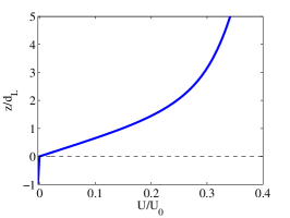
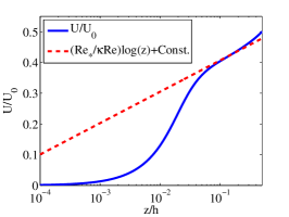
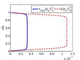
Figure 3: The base-flow variables for $Re=8000$, $m=55$, $r=1000$, and $\delta=1/50$. Subfigure (a) shows the velocity profile in the liquid and the gas, with distances normalized on the liquid-film thickness; subfigure (b) shows the development of a logarithmic profile near the centreline of the gas domain. Subfigure (c) shows the spatial dependence of the turbulent shear stress and kinetic energy.

Computation of $z_{\mathrm{t}}$:

In Sec. II, we introduced the turbulent and advective timescales. These timescales vary in the normal direction. Close to the interface, the frequency of eddy turnovers is $T_{\mathrm{t}}^{-1}$, which is large compared to the advection frequency $T_{\mathrm{a}}$. Far from the interface, the magnitude of these frequencies is reversed. Crossover occurs at $z_{\mathrm{t}}$, which is determined as the root of the equation

$$\frac{\alpha^{-1}}{\left|U\left(z_{\mathrm{t}}\right)-c\left(\alpha\right)\right|}=\frac{\kappa Re}{Re_{*}}z_{\mathrm{t}},$$ (23)

Typically, $c_{\mathrm{r}}\gg c_{\mathrm{i}}$, and negligible error is incurred by replacing $c$ by $c_{\mathrm{r}}$ in Eq. (23). Making this replacement, we can readily find a lower bound for $z_{\mathrm{t}}$:

$$Re_{*}\alpha^{-1} = \kappa z_{\mathrm{t}}\,Re\left|U\left(z_{\mathrm{t}}\right)-c_{\mathrm{r}}\right|,$$

$$\leq \kappa z_{\mathrm{t}}\,Re\,U\left(z_{\mathrm{t}}\right),$$

$$\leq \kappa Re_{*}^{2}z_{\mathrm{t}}^{2},$$

hence

$$z_{\mathrm{t}}\geq\sqrt{\frac{1}{\kappa Re_{*}\alpha}}.$$ (24)

When the wave speed $c_{\mathrm{r}}$ is small, the bound (24) sharpens. Moreover, we have verified that the propagation speed $c_{\mathrm{r}}$ is not affected by the turbulence modelling (e.g., Fig. 11 (b)), and thus the computation of $z_{\mathrm{t}}$

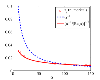
Figure 4: The crossover height $z_{\mathrm{t}}$ as a function of wavenumber for $Re=8000$. The wavelength $\alpha^{-1}$ is shown for comparison.

can be carried out using the model without the perturbation turbulent stresses (PTS). In Fig. 4 we have done precisely this: the scale $z_{\mathrm{t}}$ is computed and the bound (24) is found to be sharp. The scale $\alpha^{-1}$, which determines the spatial extent of the streamfunction, is shown for comparison. For all but the largest $\alpha$-values (shortest wavelengths), the crossover height $z_{\mathrm{t}}$ lies in a region where the streamfunction is non-negligible. Thus, we expect the streamfunction to ‘feel’ the effects of rapid distortion. Note finally that the computation of the scale $z_{\mathrm{t}}$ enables us to develop an interpolation function $\mathcal{I}\left(z\right)$, specifically, we take

$$\mathcal{I}\left(z\right)=1-e^{-\left(z/z_{\mathrm{t}}\right)^{2}},$$ (25)

in the gas. The exponent is taken to be $2$ to guarantee that the turbulent effects vanish strongly at the interface: since the flat-interface state has this property, it is reasonable to assign the same property to the perturbed state.

IV.2 Linear-stability analysis

We carry out a stability analysis around the base state just constituted for $Re=8000$, $Fr=10^{-5}$, and $S=10^{-3}$. The density and viscosity ratios are chosen such that the stability analysis models an air-water system under

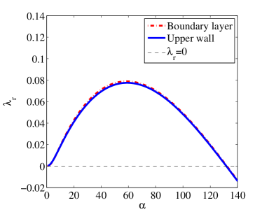
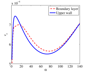
Figure 5: (a) The growth rate in the thin-film case, with $Re=8000$ (solid line). The wavenumber is normalized by the film thickness $d_{L}$, rather than the gas-domain thickness $d_{G}$, and $d_{G}/d_{L}=50$. The difference between the PTS wave and the non-PTS wave is so small as to be negligible, and is not shown here; (b) The wave speed in the thin-film case (solid line). A comparison with a boundary-layer base state with no upper plate is shown (dashed-dotted lines).

standard conditions $m=55$, $r=1000$. These Reynolds, inverse Froude, and inverse Weber numbers are chosen to correspond to typical air-water conditions for a liquid-film thickness $d_{L}=d_{G}/50$. We examine the growth rate of the disturbance with and without the effects of the PTS, and the results are shown in Fig. 5, where we also plot the wave speed. The inclusion of the PTS has little effect on the growth rate in this case, except at long wavelengths. The trend in the dispersion curve for the PTS wave shows a tiny downward shift in the growth rate relative to the non-PTS wave. The maximum growth rate occurs at $\alpha\approx 60$. Since we have non-dimensionalized on the gas-layer height, this corresponds to a wavelength $\ell/d_{L}\approx 2\pi\delta/\alpha=2\pi\times\left(50/60\right)$, that is, a wavelength greater than, but comparable to the liquid film thickness. Finally, we note that our finding that the maximum growth rate occurs at a wavelength comparable to the liquid-film thickness is similar to results obtained elsewhere for thin liquid films. The u-shaped trough in the wave-speed diagram is also characteristic of thin-film flow: we have observed it by reproducing the work of Miesen and Boersma Miesen1995 , and extracting the wave speed from the stability analysis, in addition to the growth rate. Our inclusion of an upper plate has little or no effect on the results: this can be seen by comparing the data in Fig. 5 with a true boundary layer, at the same parameter values (in particular, at the same liquid Reynolds number). This is shown by the broken-line curves in Fig. 5, where the boundary-layer stability analysis is conducted according to the framework of Miesen and Boersma Miesen1995 .

Figure 5 implies that the PTS have little effect on the growth rate at the Reynolds number considered ($Re=8000$). This can be explained by studying the form of the rapid-distortion equations (14d) and (14e): here the stress terms are damped not only by the decay function $\mathcal{I}\left(z/z_{\mathrm{t}}\right)$, but also by the equilibrium turbulent kinetic energy function $q\left(z\right)$, which is zero at the interface. For now, let us take it on trust that the instability in Fig. 5 is due to the viscosity-contrast mechanism (we verify this in Tab. 1). Then, the instability is governed by conditions at the interface and in the viscous sublayer, $z\leq Re_{*}^{-1}$. This is precisely the region in which $q\left(z\right)$ is damped to zero. Thus, in the region $z\leq Re_{*}^{-1}$ where the growth rate is determined, rapid distortion plays no role, and therefore, does not affect the growth rate. A forteriori, the PTS play no role in determining the growth rate for this particular class of instability. Nevertheless, there exists a further aspect of the problem where the PTS do alter the features of the disturbance significantly, namely the shape of the streamfunction in a zone far from the interface. Indeed, we shall find that the far-field streamfunction has an oscillatory structure that propagates far into the gas core. The existence of these oscillations casts doubt on whether the structure and statistics of the turbulence near non-linear interfacial waves is similar to that for a wall region. Ultimately, this must be confirmed by accurate numerical simulation.

We investigate the spatial structure of the perturbation velocity for wavenumbers $\alpha=15$ and $\alpha=60$; the results are shown in Figs. 6 and 7.

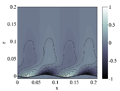
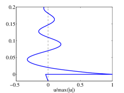
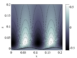
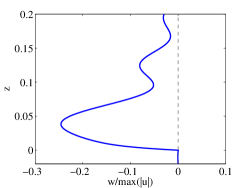
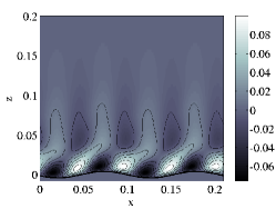
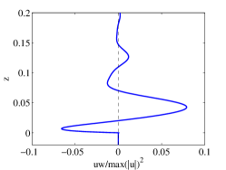
Figure 6: Flow field structure for $\alpha=15$. Subfigures (a) and (b) show the streamwise velocity field and a profile at $x=0$; subfigures (c) and (d) show the normal velocity field and a profile at $x=0$; subfigures (e) and (f) show the pre-averaged version of the wave Reynolds stress, namely the field $uw$, and its profile at $x=0$. In each case, we have normalized the velocities by $\max|u|$.

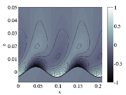
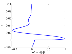
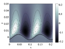
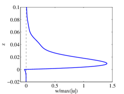
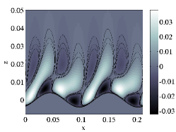
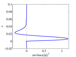
Figure 7: Flow field structure for $\alpha=60$. Subfigures (a) and (b) show the streamwise velocity field and a profile at $x=0$; subfigures (c) and (d) show the normal velocity field and a profile at $x=0$; subfigures (e) and (f) show the pre-averaged version of the wave Reynolds stress, namely the field $uw$, and its profile at $x=0$. In each case, we have normalized the velocities by $\max|u|$.

The effect of the rapid distortion on the flow is visible at $\alpha=15$, and almost negligible at $\alpha=60$. For $\alpha=15$, the streamfunction extends into the rapid-distortion domain, and the wave and the turbulence interact. This gives rise to an oscillatory structure in the velocity field, in the normal direction, as shown in Figs. 6 (b) and (d). This structure also

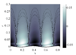
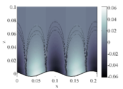
Figure 8: The pressure distribution for $\alpha=15$, (a), and $\alpha=60$, (b), normalized by $\max|u|$, the maximum streamwise perturbation velocity.

manifests itself as streaks, shown in Fig. 6 (a), which are inclined at an acute angle relative to the interface. These oscillatory structures are all but invisible in the $\alpha=60$ case (Fig. 7).

We plot the pressure distribution in Fig. 8. The minimum pressure is almost exactly out of phase with the interfacial variation at $\alpha=15$, while at $\alpha=60$ the pressure minimum is shifted slightly downstream of the free-surface maximum. The co-incidence of the pressure minimum and the free-surface maximum is explained by Bernoulli’s principle, since the gas viscosity is small. The in-phase component of the pressure at $\alpha=60$ is a consequence of the so-called quasi-separated sheltering Benjamin1958 ; Boomkamp1997 , wherein the viscous sublayer creates a wake downstream of the crest, which reduces the pressure fluctuation there.

The other phase relationships, namely those between the velocity at the interface and the interfacial disturbance can also be understood quite readily. The normal component of the velocity possesses successive extrema (maxima or minima). The first set of extrema is located at the surface $z=0$, and can be understood by examination of the kinematic condition, which in the moving frame of reference is simply $\partial\eta/\partial t=w$ at the interface. Upstream of a wave crest that is propagating from left to right ($c_{\mathrm{r}}>0$), the interfacial height decreases in time, which implies that the velocity $w$ is negative there, while downstream of the wave crest, the vertical velocity component is positive. Moreover, since $w=\Re\left[i\alpha e^{i\alpha\left(x-ct\right)}\phi\right]$, and $u=\Re\left[e^{i\alpha\left(x-ct\right)}\left(d\phi/dz\right)\right]$, there is a $\pi/2$ phase difference between $u$ and $w$, and thus the structure of the streamwise velocity can be understood simply as a phase shift relative to the normal velocity, in order to satisfy the continuity condition.

Finally, we make use of an energy-decomposition to pinpoint the source of the instability.

$\alpha=15$	$KIN_{L}$	$KIN_{G}$	$REY_{L}$	$REY_{G}$	$DISS_{L}$	$DISS_{G}$	$TURB$	$NOR$	$TAN$
PTS	0.97	0.03	0.02	9.21	-0.20	1.35	0	0.000	1.000
No PTS	0.005	0.012	-0.001	-0.185	-0.019	-0.738	-0.039	0.000	1.000

$\alpha=60$	$KIN_{L}$	$KIN_{G}$	$REY_{L}$	$REY_{G}$	$DISS_{L}$	$DISS_{G}$	$TURB$	$NOR$	$TAN$
No PTS	0.008	0.011	-0.002	-0.089	-0.024	-0.863	0	-0.004	1.000
PTS	0.007	0.011	-0.002	-0.103	-0.023	-0.832	-0.018	-0.004	1.000

Table 1: Energy budget for the thin-film flow, normalized on the tangential term.

This decomposition or budget is obtained from the RANS equations, and was introduced by Boomkamp and Miesen Boomkamp1996 :

$$r_{j}\left(\frac{\partial}{\partial t}\delta\bm{u}_{j}+\bm{U}_{j}\cdot\nabla\delta\bm{u}_{j}+\delta\bm{u}_{j}\cdot\nabla\bm{U}_{j}\right)=\nabla\cdot\delta\mathsf{T}^{(j)}-r_{j}\nabla\cdot\delta\mathsf{r}^{(j)}$$ (26a)

$$\delta\mathsf{T}=\left(\begin{array}[]{cc}-\delta\pi&\mu\left(\partial_{x}\delta w+\partial_{z}\delta u\right)\\ \mu\left(\partial_{x}\delta w+\partial_{z}\delta u\right)&-\delta\pi\end{array}\right),\qquad\delta\mathsf{r}=\left(\begin{array}[]{cc}-\delta\mathsf{r}_{11}+\delta\mathsf{r}_{22}&-\delta\mathsf{r}_{12}\\ -\delta\mathsf{r}_{12}&0\end{array}\right)$$ (26b)

$$\nabla\cdot\bm{u}_{j}=0,$$ (26c)

which we multiply by the velocity $$\delta\bm{u}_{j}$$ and integrate over space. We obtain the following balance equation:

$$\sum_{j=L,G}\mathrm{KIN}_{j}=\sum_{j=L,G}\mathrm{REY}_{j}+\sum_{j=L,G}\mathrm{DISS}_{j}+\sum_{j=L,G}\mathrm{TURB}_{j}+\mathrm{INT},$$ (26d)

where

$$\mathrm{KIN}_{j} = \tfrac{1}{2}\frac{\mathrm{d}}{\mathrm{d}t}\int dx\int dz\,r_{j}\delta\bm{u}_{j}^{2},$$ (26e)

$$\mathrm{REY}_{j} = -r_{j}\int dx\int dz\,\delta u_{j}\delta w_{j}\frac{\mathrm{d}U_{j}}{\mathrm{d}z},$$ (26f)

$$\mathrm{DISS}_{j} = -\frac{m_{j}}{Re}\int dx\int dz\,\left[2\left(\frac{\partial{}}{\partial{x}}\delta u_{j}\right)^{2}+\left(\frac{\partial}{\partial z}\delta u_{j}+\frac{\partial}{\partial x}\delta w_{j}\right)^{2}+2\left(\frac{\partial}{\partial z}\delta w_{j}\right)^{2}\right],$$ (26g)

$$\mathrm{TURB}_{j} = \delta_{j,G}\bigg{\{}r\int dx\int dz\,\left[\delta\mathsf{r}\frac{\partial}{\partial x}\delta u+\delta\mathsf{r}_{12}\left(\frac{\partial}{\partial z}\delta u+\frac{\partial}{\partial x}\delta w\right)\right]\bigg{\}}.$$ (26h)

Additionally,

$$\mathrm{INT}=\int dx\,\left[\delta u_{L}\delta\mathsf{T}_{L,zx}+\delta w_{L}\mathsf{T}_{L,zz}\right]_{z=0}-\int dx\,\left[\delta u_{G}\delta\mathsf{T}_{G,zx}+w_{G}\delta\mathsf{T}_{G,zz}\right]_{z=0},$$

which is decomposed into normal and tangential contributions,

$$\mathrm{INT}=\mathrm{NOR}+\mathrm{TAN},$$

where

$$\mathrm{NOR}=\int dx\,\left[\delta w_{L}\delta\mathsf{T}_{L,zz}-\delta w_{G}\delta\mathsf{T}_{G,zz}\right]_{z=0},$$

and

$$\mathrm{TAN}=\int dx\,\left[\delta u_{L}\delta\mathsf{T}_{L,zx}-\delta u_{G}\delta\mathsf{T}_{G,zx}\right]_{z=0}.$$

The results of this study are given in Tab. 1. We find in each case that the tangential term is the source of the instability. This can be re-written as

$$\mathrm{TAN}=U_{G}^{\prime}\left(0\right)\left(m-1\right)\int_{0}^{\ell}\delta T_{xz}\left(x,0\right)\eta\left(x\right)dx,$$

which is positive when $m>1$, and when the viscous shear stress $\delta T_{xz}\left(x,0\right)$ is less than $\pi/2$ out-of-phase with the interfacial variation. Thus, the instability is driven by the viscosity contrast $m>1$.

IV.3 A simplified calculation to elucidate the rapid-distortion effects

To understand the effects of rapid distortion on the structure of the streamfunction, rather than on the stability of the system, we resort to a highly simplified model, where analytical progress is possible. This model possesses as its solution the oscillatory structures visible in Figs. 6 and 7. We perform a linear-stability analysis around the base state

$$U=\begin{cases}mz,&-1\leq z\leq 0,\\ z,&0\leq z\leq b,\\ b,&z\geq b.\end{cases}$$ (27)

We make use of the following Orr–Sommerfeld and PTS equations:

$$i\alpha r\left(mz-c\right)\left(\mathrm{D}^{2}-\alpha^{2}\right)\phi_{L}=\frac{m}{Re}\left(\mathrm{D}^{2}-\alpha^{2}\right)^{2}\phi_{L},\qquad-1\leq z\leq 0,$$ (28a)

$$i\alpha\left(z-c\right)\left(\mathrm{D}^{2}-\alpha^{2}\right)\phi_{G}=\frac{1}{Re}\left(\mathrm{D}^{2}-\alpha^{2}\right)^{2}\phi_{G},\qquad 0\leq z\leq b,$$ (28b)

$$i\alpha\left(b-c\right)\left(\mathrm{D}^{2}-\alpha^{2}\right)\phi_{G}=\frac{1}{Re}\left(\mathrm{D}^{2}-\alpha^{2}\right)^{2}\phi_{G}+\left(\mathrm{D}^{2}+\alpha^{2}\right)\tau,\qquad z\geq b,$$ (28c)

$$i\alpha\left(U_{0}-c\right)\tau=-q_{\infty}\left(\alpha_{1}\mathrm{D}^{2}\phi_{G}+\alpha_{2}\alpha^{2}\phi_{G}+i\alpha\alpha_{3}\mathrm{D}\phi_{G}\right),$$ (28d)

where now $q_{\infty}$, the constant turbulent kinetic energy in the far field, can be thought of as parametrizing the PTS. Given a set of boundary and interfacial conditions, it is possible to obtain a closed-form solution to this set of equations, in terms of exponentials and integrals of Airy functions DrazinReidBook ; abram_stegun . Our goal here, however, is simply to elucidate the oscillatory nature of the solution found in the full analysis. To that end, we take a characteristic value of the wave speed $c$, and obtain a solution to the system (28d) in the far field $z\geq b$. There, the solution is $\phi_{G}=e^{\varsigma z}$, where $\varsigma$ solves a fourth-order polynomial equation:

$$\left(1+i\alpha_{1}Re_{q}\right)\left(\varsigma/\alpha\right)^{4}-\alpha_{3}Re_{q}\left(\varsigma/\alpha\right)^{3}+\left[i\left(\alpha_{1}+\alpha_{2}\right)Re_{q}-2-iRe_{b}\right]\left(\varsigma/\alpha\right)^{2}\\ -\alpha_{3}Re_{q}\left(\varsigma/\alpha\right)+iRe_{q}\alpha_{2}+1+iRe_{b}=0,$$ (29)

where

$$Re_{q}=\frac{Req_{\infty}}{\alpha\left(b-c\right)},\qquad Re_{b}=\frac{Re\left(b-c\right)}{\alpha}.$$

When $b\gg|c|$, we have the condition $|Re_{b}|\gg|Re_{q}|$, and we can treat $|Re_{q}|^{-1}$ as a small expansion parameter. The lowest-order solution of Eq. (29) is then $\varsigma^{2}=\alpha^{2}$ or $\alpha^{2}+i\alpha Re\left(b-c\right)$, and the rapid-distortion effects appear at first order. In fact,

$$\varsigma=\begin{cases}\varsigma_{1}=-\alpha\left[1+\frac{q_{\infty}}{\left(b-c\right)^{2}}\left(\alpha_{1}+\alpha_{2}-i\alpha_{3}\right)\right],\\ \varsigma_{2}=-\alpha\sqrt{iRe_{b}}\left[1+\frac{q_{\infty}}{\left(b-c\right)^{2}}\frac{\alpha_{1}Re_{b}}{2}\right],\qquad|Re_{b}|\gg 1.\end{cases}$$ (30)

Note, however, that the rapid-distortion effects appear non-perturbatively in $\varsigma_{2}$ for sufficiently large values of $|Re_{b}|q_{\infty}$. The exact condition is $\alpha_{1}q_{\infty}Re_{b}/\left(b-c\right)^{2}=O\left(1\right)$, which equates to

$$\alpha\apprle\frac{\alpha_{1}q_{\infty}Re}{|b-c|}.$$ (31)

Using typical values for the thin-film waves ($Re=10^{4}$, $q_{\infty}=10^{-3}$, $|b-c|=10^{-1}$, $\alpha_{1}=10^{-1}$), we expect rapid distortion to affect the streamfunction at lowest order when $\alpha\apprle 10$. This analysis is verified by the streamfunction plots in Fig. 9, using $q_{\infty}=10^{-3}$, where we take $b=0.25$, and $Re=8000$. The coefficients $\alpha_{1}$, $\alpha_{2}$, and $\alpha_{3}$ are taken from Sec. II.3, while the $c$-values are taken from Fig. 5 at $\alpha=10$ and $\alpha=60$.

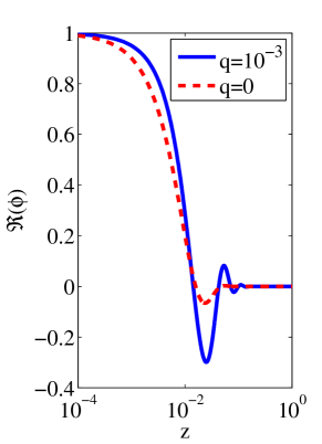
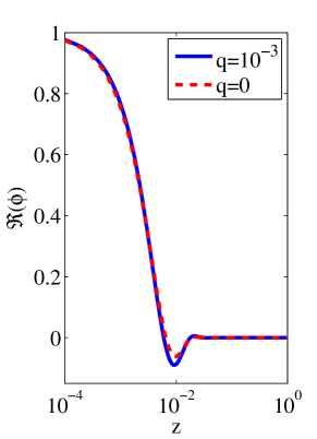
Figure 9: Far-field streamfunction for the simplified model, $Re=8000$, $b=0.25$, and $c$ taken from Fig. 5. The wavenumber is $\alpha=10$ in (a) and $\alpha=60$ in (b). At longer wavelengths, the rapid distortion induces an oscillation in the streamfunction, seen in the comparison between the $q_{\infty}=0$ and $q_{\infty}=10^{-3}$ curves in (a). At shorter wavelengths, this effect vanishes (see (b)). This agrees qualitatively with the streamfunction pattern in the full model.

In Fig. 9 (a) we compare the far-field streamfunction associated with the mode $\varsigma_{2}$ with and without the PTS at $\alpha=10$. There is a clear difference between the two cases, while the difference between the two modes associated with $\varsigma_{1}$ is negligible (the difference is small and the plot is not shown). This is consistent with the analysis in Eqs. (30) and (31). The consistency extends to the $\alpha=60$ case (Fig. 9 (b)), where there is little difference between the $\varsigma_{1}$ and $\varsigma_{2}$ streamfunctions. The enhanced oscillations in the streamfunction visible in Fig. 9 (a) are similar to those obtained by Zaki and Saha Zaki2009 in their study of the interaction between disturbances in the free stream and the boundary layer. There, the authors used the continuous-spectrum Orr–Sommerfeld equation as a model, and the qualitative agreement between our findings and theirs further vindicates our results.

Note finally that there is another way for the rapid distortion to make itself felt at zeroth order in the polynomial equation (29). When $b\approx c_{\mathrm{r}}$, the speed $b-c$ is small, and $|Re_{q}|\gg|Re_{b}|$. By treating $|Re_{b}|^{-1}$ as an expansion parameter, we obtain the zeroth-order polynomial to solve:

$$i\alpha_{1}\left(\varsigma/\alpha\right)^{4}-\alpha_{3}\left(\varsigma/\alpha\right)^{3}+i\left(\alpha_{1}+\alpha_{2}\right)\left(\varsigma/\alpha\right)^{2}-\alpha_{3}\left(\varsigma/\alpha\right)+i\alpha_{2}=0.$$

In this case, the oscillatory term in the streamfunction $\phi=e^{\Re\left(\varsigma\right)z}e^{i\Im\left(\varsigma\right)z}$ is due mostly to the rapid distortion, and the contribution from the oscillation coming from the base flow is a perturbation. This is made manifest when we write down the closed-form solution of the equation that exists when $\alpha_{3}=0$:

$$\varsigma=\pm\alpha\sqrt{-\tfrac{1}{2}\left(1+\frac{\alpha_{2}}{\alpha_{1}}\right)\pm\tfrac{1}{2}\sqrt{\left(\frac{\alpha_{2}}{\alpha_{1}}\right)^{2}+2\left(\frac{\alpha_{2}}{\alpha_{1}}\right)-3}}.$$

We expect this last mechanism to be important for fast waves, that is, for a case in which the equation $b-c_{\mathrm{r}}\left(\alpha\right)=0$ has a solution. We therefore turn our attention to a situation in which such fast waves occur.

V Results for deep-water waves

In this section we investigate the effects of turbulence on the stability of an interface separating a deep body of liquid from a gas layer that acts on the interface by a fully-developed turbulent shear flow.

V.1 Base-state determination

As before, we use a base state that mimics flow in a boundary layer, and thus, the flow is confined by a flat plate at $z=d_{G}$, a large distance from the interface. This plate moves at velocity $U_{0}$ relative to the interface. Using this framework, the basic velocity is constituted as before: the non-dimensional velocity is given by Eq. (21d), where $Re_{*}=\rho_{G}U_{*\mathrm{i}}d_{G}/\mu_{G}$, and $Re=\rho_{G}U_{0}/d_{G}$.

The eddy-viscosity and wall functions $$G \psi$$ and have their usual meaning, given by Eqs. (21b) and (21c) respectively. The sole difference between the profile in Sec. IV and that used here is in the liquid, where we make use of the following deep-water profile Zeisel2007 :

$$\tilde{U}_{L}=a\left(e^{b\tilde{z}}-1\right),$$ (32a)

where $$a b$$ and are constants to be determined. There is in fact, only one constant to determine, since the continuity of tangential stress requires that

$$m\frac{\mathrm{d}\tilde{U}_{L}}{\mathrm{d}\tilde{z}}=\frac{\mathrm{d}\tilde{U}_{G}}{\mathrm{d}\tilde{z}},\qquad\tilde{z}=0.$$ (32b)

Hence, $$mab=Re_{*}^{2}/Re a$$, and there remains a single free constant whose value is fixed in Tab 2. Thus, the liquid velocity has the reduced form

$$\tilde{U}_{L}=a\left(e^{\frac{\tilde{z}Re_{*}^{2}}{maRe}}-1\right).$$

$a$	Amplitude of drift	Not determined, although a value $a=U_{*\mathrm{i}}/(2U_{0})$
		is given in the literature Zeisel2007 .
$b$	Decay scale of the	Determined from $a$ and the viscosity contrast
	drift velocity	$m$ through the continuity of tangential stress
$C$	The kinetic energy amplitude	$C=0.55$, to agree with log-layer
	is given by $C^{-2}$ in wall units.	conditions in boundary-layer flow.
$n$	Exponent in the Van	Chosen such that the Reynolds stress and the
	Driest damping function	kinetic energy mimic wall turbulence as $z\rightarrow 0$.
$A$	Length scale in the Van	Chosen such that the linear region of the base
	Driest damping function	flow is approximately $5$ wall units in depth.

Table 2: Summary of the parameters used in Eqs. (32).

Computation of $z_{\mathrm{t}}$:

In carrying out the stability analysis, we have verified that the real part of the wave speed is affected only slightly by the turbulence modelling (less than %1), and thus the computation of $z_{\mathrm{t}}$

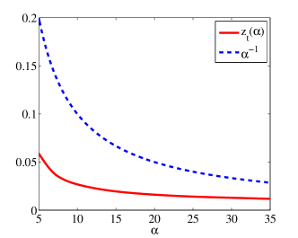
Figure 10: The crossover height $z_{\mathrm{t}}$ as a function of wavenumber for $Re=10^{5}$, $r=1000$, and $m=55$. The wavelength $\alpha^{-1}$ is shown for comparison.

can be carried out using the model without the perturbation turbulent stresses (PTS). The crossover value $z_{\mathrm{t}}$ where the turbulent and advection timescales are equal is thus determined by Eq. (23); the dependence of $z_{\mathrm{t}}$ on $\alpha$ is shown in Fig. 10, for $Re=10^{5}$. The plot is similar to Fig. 4: the streamfunction extends into the domain where rapid distortion is important, and we therefore expect to see the shape of the streamfunction adjust to take account of the wave-turbulent interactions. As before, our computation of $z_{\mathrm{t}}$ enables us to develop an interpolation function $\mathcal{I}\left(z\right)$ in the gas: we take $\mathcal{I}\left(z\right)=1-e^{-\left(z/z_{\mathrm{t}}\right)^{2}}$, and for simplicity, we replace the $\alpha$-dependent variable $z_{\mathrm{t}}\left(\alpha\right)$ its average value, obtainable from Fig. 10.

V.2 Linear-stability analysis

We carry out a stability analysis around the base state just constituted at a Reynolds number $Re=10^{5}$, and at an inverse Froude number $Fr=500$. The inverse Weber number $S$ is set to zero, a realistic assumption since the Froude number is large and thus gravity dominates over capillarity. The density and viscosity ratios are chosen such that the stability analysis models an air-water system under standard conditions: $r=1000$ and $m=55$ respectively. These Reynolds and Froude numbers are chosen such that the so-called critical-layer instability is observed. We examine the growth rate of the disturbance with and without the PTS. A description of the change in the growth rate upon adding the PTS is shown in Fig. 11. We also plot the wave speed in Fig. 11, which is unchanged by the PTS-modelling. The segment of the dispersion curve that is of interest is the short-wave limit, for which $\alpha\gg 2\pi$ (where all lengths are measured relative to the gas-layer height $d_{G}$). For longer waves, there is an interaction between the upper plate and the wave streamfunction, and the model no longer describes boundary-layer phenomena. The maximum growth rate occurs substantially above this lower cutoff

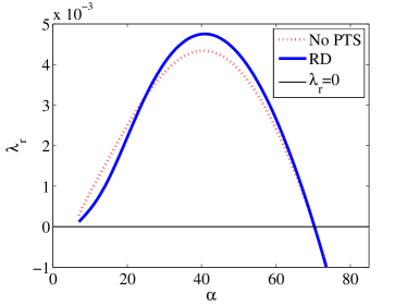
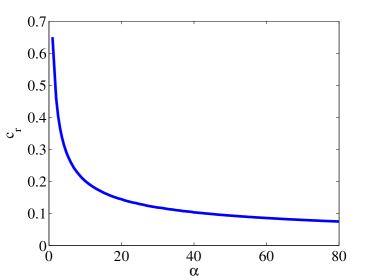
Figure 11: The growth rate and wave speed of the PTS (continuous) and non-PTS waves (dotted lines), as a function of wavenumber $\alpha$, normalized on the gas-layer thickness.

value, at a wavenumber $\alpha_{\mathrm{max}}\approx 40$, while gravity stabilizes the wave above an upper critical wavenumber $\alpha_{\mathrm{c}}\approx 70$. The location of the maximum growth rate is not changed by the PTS, although its value is shifted upwards, by about $10\%$. We do not continue the PTS dispersion curve below $\alpha=10$, since the PTS streamfunction is difficult to resolve numerically below this value. We do, however, describe the dispersion curve for the non-PTS case below this threshold in Fig. 12. There growth rate oscillates between positive and negative values. It is tempting to dismiss this as an effect of the upper plate; this is not the case however, since the effect persists upon increasing the depth of the gas layer. This anomalous region is far from the most dangerous mode, and we do not study it further.

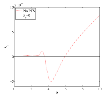
Figure 12: The growth rate at long wavelengths in the non-PTS case.

Now the structure of the flow field also changes as a consequence of the varying level of intensity of the rapid distortion, and it is to this variation that we now turn examining the perturbation velocity at different wavenumbers.

$\alpha=15$:

At this wavenumber, the wave parameters (growth rate and propagation speed) are

$$\lambda_{\mathrm{r}} = 0.0004,\qquad c_{\mathrm{r}}=0.2011,\qquad\text{with the PTS};$$

$$\lambda_{\mathrm{r}} = 0.0008,\qquad c_{\mathrm{r}}=0.2011,\qquad\text{with no PTS};$$

$$z_{\mathrm{c}} = 0.0065,$$ (33)

where $z_{\mathrm{c}}$ is the critical height, for which $U\left(z_{\mathrm{c}}\right)=c_{\mathrm{r}}$.

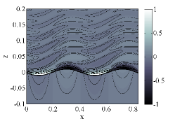
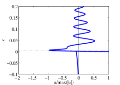
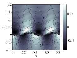
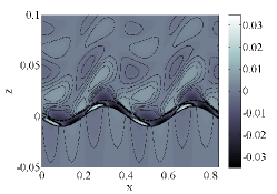
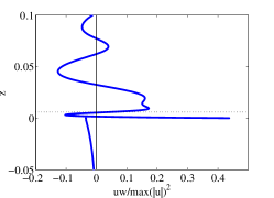
Figure 13: Flow field structure for $\alpha=15$. The critical layer is shown as a dotted line above the interface. The effects of the rapid distortion are particularly visible in subfigures (a) and (b), which display the streamwise velocity and the streamwise velocity at $x=0$, respectively. Subfigures (c) and  (d) show the normal velocity and the normal velocity at $x=0$. The effects of the rapid distortion are again visible in the pre-averaged version of the wave Reynolds stress, namely the product $uw$, shown in (e) and (f). In each case, we have normalized the velocities by $\max|u|$.

The velocity field associated with this wave is shown in Fig. 13. These figures all possess similar features, regardless of the PTS. The normal component of the velocity possesses successive extrema (maxima or minima). The first set of extrema is located at the surface $z=0$, and, as in Sec. IV, can be understood by examination of the kinematic condition, which in the moving frame of reference is simply $\partial h/\partial t=w$ at the interface. Upstream of a wave for which $c_{\mathrm{r}}>0$, the interfacial height decreases in time, implying that $w<0$ there; similarly, $w>0$ in the downstream region. In contrast to Sec. IV, there is another set of extrema located above the critical layer; this is discussed below in the context of the $\alpha=40$ wave. In addition, since $w=\Re\left[i\alpha e^{i\alpha\left(x-ct\right)}\phi\right]$, and $u=\Re\left[e^{i\alpha\left(x-ct\right)}\left(d\phi/dz\right)\right]$, there is a $\pi/2$ phase difference between $u$ and $w$, and thus the structure of the streamwise velocity can be understood simply as a phase shift relative to the normal velocity. The phase relationships discussed combine to give a distinctive phase relationship for the pressure field, shown in Fig. 14. In particular, at maximum growth, the pressure and the interfacial wave are approximately $\pi/4$ out of phase. Furthermore, the far-field structure of the PTS and non-PTS waves differ by the presence in the former case of successive velocity extrema, succeeding the one associated with the critical layer. These are due to the effects of the rapid distortion on the wave-induced motion, and are visible as velocity ‘streaks’ in the streamwise direction (see Fig. 13 (a)); these streaks are tilted forwards in the direction of the base flow.

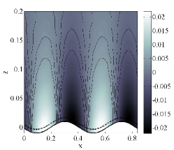
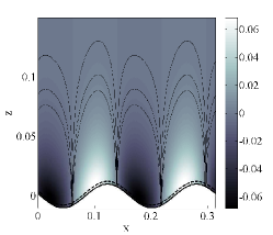
Figure 14: The pressure distribution for $\alpha=15$, (a), and $\alpha=40$, (b), normalized by $\max|u|$. The critical layer is shown as a dotted line above the interface.

$\alpha=40$:

At this wavenumber, the wave parameters are

$$\lambda_{\mathrm{r}} = 0.0043,\qquad c_{\mathrm{r}}=0.1033,\qquad\text{with the PTS};$$

$$\lambda_{\mathrm{r}} = 0.0047,\qquad c_{\mathrm{r}}=0.1033,\qquad\text{with no PTS};$$

$$z_{\mathrm{c}} = 0.0023;$$ (34)

We present an energy budget for the case $\alpha=40$ in Tab. 3, which is calculated from the streamfunction using the balance law formulated in Eq. (26). The energy terms are further normalized such that the total energy of the PTS wave sums to unity.

$\alpha=40$	$KIN_{L}$	$KIN_{G}$	$REY_{L}$	$REY_{G}$	$DISS_{L}$	$DISS_{G}$	$TURB$	$NOR$	$TAN$
PTS	0.99	0.01	-0.04	4.15	-0.88	-2.53	0.04	-2.06	2.32
No PTS	0.99	0.01	-0.01	2.81	-0.62	-1.76	0	-1.01	1.61

Table 3: The energy budget for the deep-water waves at $\alpha=40$, near maximal growth.

The two energy budgets possess only small relative differences, in spite of the large difference between the associated growth rates. This is because the kinetic energy possesses contributions both from $c_{\mathrm{r}}$ and $c_{\mathrm{i}}$, and while the difference in $c_{\mathrm{i}}$ is large, the difference in $c_{\mathrm{r}}$ is small, and $c_{\mathrm{r}}\gg c_{\mathrm{i}}$. Thus, the precise mechanism of excess instability is not visible from the energy budget. Nevertheless, the energy budget does indicate that the maximum destabilizing term is $REY_{G}$, and we therefore study the wave Reynolds stress:

$$\tau_{\mathrm{wave}}^{(j)}\left(z\right)=-r_{j}\int_{0}^{2\pi/\alpha}\delta u_{j}\left(x,z\right)\delta w_{j}\left(x,z\right)dx,$$

The sum $REY_{G}$ is thus

$$REY_{G}=\int_{0}^{1}\tau_{wave}^{G}\left(z\right)\frac{\mathrm{d}U}{dz}dz$$

and thus the wave Reynolds stress represents the energy associated with the power $REY_{G}$. We plot the wave Reynolds stress in Fig. 15.

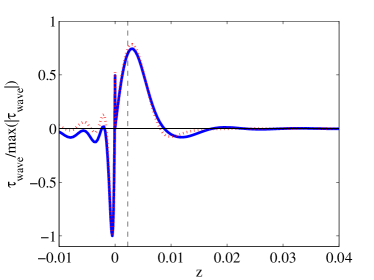
Figure 15: The unit-normalized wave Reynolds stress for $\alpha=40$. The critical layer is at $z_{\mathrm{c}}=0.0022$, shown in the figure. The stress function for the non-PTS wave is given by the dotted line, while the continuous curve indicates the PTS wave. The PTS stress function possesses an oscillatory structure in the gas layer.

The peak in $\tau_{\mathrm{wave}}$ next to the critical height $z_{\mathrm{c}}$ represents a net transfer of energy from the mean flow $U\left(z\right)$ into the perturbation flow. This is present in both the PTS wave and the non-PTS wave and indicates that the instability is a critical-layer or Miles instability. Note, however that the PTS wave possesses an oscillation that propagates into the bulk gas flow, due to the interaction between the turbulence and the interface.

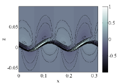
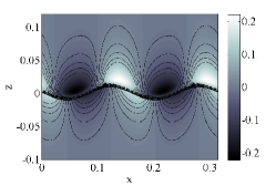
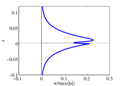
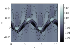
Figure 16: Flow field structure for $\alpha=40$. The critical layer is shown as a dotted line above the interface. The effects of the rapid distortion on the structure of the flow field no longer visible. The streamfunction decays in the bulk of the gas more rapidly than in the $\alpha=10$ case (as evidenced by a comparison between Figs. 16 (d) and 13 (d)). Subfigures (a) and (b) show the streamwise velocity and a profile at $x=0$; subfigures (c) and (d) show the normal velocity and a profile at $x=0$; subfigures (e) and (f) show the pre-averaged version of the wave Reynolds stress, namely the product $uw$. In each case, we have normalized the velocities by $\max|u|$.

In contrast to the $\alpha=10$ case, the velocity fields in Fig. 16 possess the same structure, regardless of the PTS, and neither the oscillation nor the streamwise streaks are visible. This is consistent with the predictions of the piecewise-constant model in Sec. IV.3.

Finally, in Figs. 17 and 18 we plot the turbulent kinetic energy and Reynolds stresses at $\alpha=15$ and $40$ respectively. These are an order of magnitude smaller than the wave Reynolds stress $uw$, confirming the importance of the latter term, relative to the turbulent variables. Note that for the smaller of the two $\alpha$-values, the maximum values of the turbulent variables lie close to the critical layer (Fig. 17), while for the larger $\alpha$-value, the maximum lies far above the critical height (Fig. 18). This is consistent with the growth-rate curve in Fig. 11, where the relative change in the growth rate (based on a comparison between the PTS no-PTS curves)

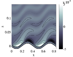
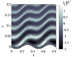
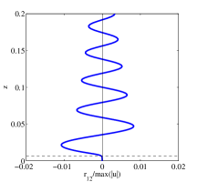
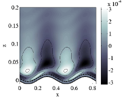
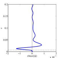
Figure 17: Turbulence variables at $\alpha=15$. The critical layer is shown as a dotted line above the interface. (a) and (b) show the turbulent kinetic energy; (c) and (d) show tangential Reynolds stress, while (e) and (f) show the normal Reynolds stress. We have normalized the perturbed turbulent quantities by $\max|u|$, the maximum of the perturbed velocity.

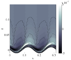
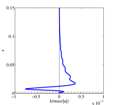
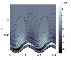
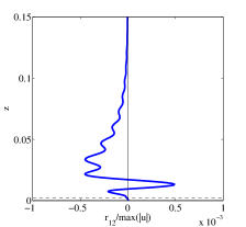
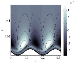
Figure 18: Turbulence variables at $\alpha=40$. The critical layer is shown as a dotted line above the interface. (a) and (b) show the turbulent kinetic energy; (c) and (d) show tangential Reynolds stress, while (e) and (f) show the normal Reynolds stress. We have normalized the perturbed turbulent quantities by $\max|u|$, the maximum of the perturbed velocity.

was larger at smaller $\alpha$-values, suggesting an interaction between the critical-layer mechanism and the wave turbulence. For larger $\alpha$-values (in particular, close to the maximum growth rate), the relative change in the growth rate is smaller.

In summary, the behaviour of the PTS wave differs from that of the non-PTS wave. The difference is both quantitative (the growth rate shifts), and qualitative (the flow field changes, especially at longer wavelengths). At longer wavelengths, the streamwise velocity exhibits streaks due to the interaction of the wave and the turbulence. At shorter wavelengths, this effect is reduced, although the growth rate is enhanced relative to the case without the PTS.

V.3 Comparison with other work

Since we have identified the instability as a critical-layer instability, it is appropriate to compare our results with the theory of Miles. Morland and Saffman Morland1993 have developed explicit formulas that enable such a comparison. We also develop a comparison with deep-water waves based on the work of Boomkamp and Miesen in Boomkamp1996 .

In the paper of Boomkamp and Miesen Boomkamp1996 , the authors present one calculation of the wave Reynolds stress based on a boundary-layer gas profile and an exponential profile in the liquid. We perform this calculation again and construct a dispersion curve over a range of $\alpha$-values. This result is shown in Fig. 19,

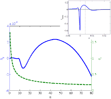
Figure 19: Comparison with the work of Boomkamp and Miesen Boomkamp1996 . The wave Reynolds stress at $\alpha$=40 is shown as in inset, with the critical layer at $z_{\mathrm{c}}=0.0044$. The growth-rate is designated by the solid curve, with a scale on the left-hand side, while the wave-speed is designated by the dashed-line curve, whose scale is on the right-hand side.

and the wave Reynolds stress calculation is given as an inset. This calculation agrees with that given by Boomkamp and Miesen. More interesting is the dispersion curve. This is qualitatively similar to those given in Figs. 11 and 12, although the gravity, surface-tension and Reynolds numbers are different. Note in particular that the growth rate switches rapidly from positive to negative values at small $\alpha$-values. This is not a finite-size effect, since it persists upon increasing the size of the computational domain and upon grid refinement. Having confirmed a qualitative similarity between the present work and a reconstruction of that of Boomkamp and Miesen, we endeavour to produce a more exact comparison. This we do by changing the parameter-values in the reconstructed work: specifically, we take $Fr=500$, $S=0$, $Re=10^{5}$, and normalize the base-state velocity such that $U_{G}\left(\tfrac{1}{2}\right)=\tfrac{1}{2}$. This facilitates an accurate comparison between our work and that of Boomkamp and Miesen. We present the comparison in Fig. 20, together with a comparison with the Miles formula.

Now the critical-layer theory of Miles Miles1957 involves the solution of the Rayleigh equation with boundary conditions at infinity, and at a wavy, impermeable wall, which is supposed to represent the interface of two fluids with a large density contrast. For this model problem, Morland and Saffman Morland1993 have derived an explicit but approximate formula for the growth rate in the case of the exponential profile

$$U=U_{\infty}\left(1-e^{-2z/\Delta}\right),$$

where for comparison we take $U_{\infty}=U_{0}/2$, and $\Delta=Re/Re_{*}^{2}$. Their approximate formula for the growth rate is

$$\lambda_{\mathrm{r}}=\frac{16\pi\alpha^{2}\Delta U_{\infty}^{2}}{rc_{0}\left(2+\alpha\Delta\right)^{2}\left(4+\alpha\Delta\right)^{2}}\left(1-\frac{c_{0}}{U_{\infty}}\right)^{2+\alpha\Delta},\qquad c_{0}=\sqrt{\frac{g}{\alpha}}.$$ (35)

We plot $\lambda_{\mathrm{r}}$ against $c_{0}$ for this simplified system, and compare the result with the relationship we have obtained between $\lambda_{\mathrm{r}}$ and $c_{\mathrm{r}}$. The results are shown in Fig. 20. There is excellent agreement among the three curves shown, although

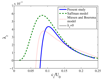
Figure 20: Comparison between our work, the analytical approximation of Morland and Saffman Morland1993 , and a reconstruction of the work of Boomkamp and Miesen Boomkamp1996 . There is good agreement between all three models, although the analytical formula breaks down at small wave speeds, where surface tension exerts a stabilizing influence on the growth rate.

the analytical curve corresponding to the formula (35) breaks down at small wave speeds, where surface tension stabilizes the system. Nevertheless, the form of curves in Fig. 20 is the same in each case, which, in addition to the energy budgets and Fig. 15, provides confirmation of the critical-layer nature of the instability.

There are also some DNS results available in this field for comparison. In particular, we focus on the work of Sullivan et al. Sullivan1999 and compare our results with DNS results found therein. While a direct comparison is not possible, since the work of Sullivan et al. is for flow over a wavy wall, there our some qualitative similarities between the two two studies.

Sullivan et al. identify slow-wave and fast-wave cases. Thus, we make a comparison between our Fig. 7 and Fig. 17 in the work of Sullivan et al., which is for slow waves, and for a critical layer that that plays no role in the dynamics. There is good qualitative agreement between these to sets of figures, although evidence of rapid distortion is absent in both cases. Next, we compare a fast-wave scenario, namely our Figs. 13 and 16 with Fig. 19 in Sullivan et al.. Again, there is good qualitative agreement between these sets of figures, in particular for the phase relationships at the interface (the corresponding results for the phase relationships of the pressure field also show good agreement). There is some evidence of rapid distortion in the secondary extrema in the streamwise velocity in Fig. 19 (a) of Sullivan et al., although this is not conclusive: this comparison implies that our model over-estimates this effect. That said, these secondary oscillations cannot be reproduced by our linear theory if we neglect the PTS.

V.4 Transition to the viscosity-contrast instability

We have investigated two types of interfacial instability, and the effects of the PTS thereon. On the energy-budget side, these waves are distinguished by the energy term that produces the instability: either the viscosity-jump mechanism, or the critical-layer mechanism. On the turbulence side, they are distinguished by the wave speed: the viscosity-jump waves are slow, while the critical-layer waves are fast. This separation of speeds leads to distinct properties with respect to the PTS. We want to find a transition from one regime to another: this can be achieved by changing the gravity number $Fr$ (inverse Froude number). We study the deep-water waves again. We obtain the dispersion curve for a range of gravity numbers, and at fixed Reynolds number, and reduce the gravity number. This can be achieved either by changing the degree of density stratification, the gas-layer thickness, or by changing the shear velocity $U_{0}$:

$$Fr=\frac{g\left(\rho_{L}-\rho_{G}\right)d_{G}}{\rho_{G}U_{0}^{2}}.$$

The dispersion curves are shown as a function of gravity number, expressed as a fraction of $Fr_{0}=500$ in Fig. 21. The growth rate changes shape as the gravity number is decreased: the high-gravity number shape is similar to that observed in this section for critical-layer

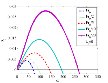
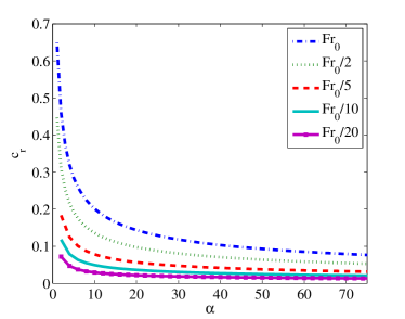
Figure 21: The growth rate and wave speed in the absence of the PTS, as a function of gravity number, for $Fr_{0}=500$ and $Re=10^{5}$. The instability changes character as the gravity number is decreased.

waves, while the low-gravity number shape is similar to that observed in Sec. IV for viscosity-stratified waves. The plot of wave speed in Fig. 21 (b) indicates that the high-gravity number waves are fast while the low-gravity number waves are slow. Going to larger $Fr$-values stabilizes the interface completely, although we have not shown this effect in Fig. 21. For each dispersion curve, we obtain the energy budget associated with maximum growth, given in Tab. 4. We observe a transition from critical-layer to viscosity-driven instability, with decreasing gravity number. The term $TAN$ represents only a small positive contribution at high $Fr$-values, while at low $Fr$-values, it is the dominant positive contribution. The presence of the PTS does little to modify this partition of energy between the tangential and $REY_{G}$ terms.

This mechanism for modifying the character of the instability could be applied to the thin-film case, with one reservation. To move the critical layer sufficiently far into the bulk gas domain such that $U^{\prime\prime}\left(z_{\mathrm{c}}\right)$ is significant, it is necessary to increase the Reynolds number. This in turn will destabilize the liquid through an internal mode, which necessitates the turbulent modelling both of the base liquid flow, and of the liquid PTS, which is beyond the scope of the present work. However, by naively retaining the linear profile in the liquid, we have observed a switch between critical-layer and viscosity-stratified waves in the thin-film case, through a suitable modification of the gravity and Reynolds numbers ($Re=10^{6}$, $Fr=0.1$, maximum growth rate at $\alpha=25$).

$Fr$	$REY_{L}$	$REY_{G}$	$DISS_{L}$	$DISS_{G}$	$TURB$	$NOR$	$INT$
$Fr_{0}$	0.00	1.75	-0.39	-1.10	0.00	-0.58	1.00
$\tfrac{1}{2}Fr_{0}$	-0.01	0.42	-0.32	-0.74	0.00	-0.17	1.00
$\tfrac{1}{5}Fr_{0}$	0.00	0.07	-0.19	-0.72	0.00	-0.04	1.00
$\tfrac{1}{10}Fr_{0}$	0.00	-0.02	-0.14	-0.74	0.00	-0.04	1.00
$\tfrac{1}{20}Fr_{0}$	0.00	-0.07	-0.09	-0.77	0.00	-0.05	1.00

$Fr$	$REY_{L}$	$REY_{G}$	$DISS_{L}$	$DISS_{G}$	$TURB$	$NOR$	$INT$
$Fr_{0}$	-0.02	1.79	-0.38	-1.09	0.02	-0.89	1.00
$\tfrac{1}{2}Fr_{0}$	-0.01	0.42	-0.32	-0.74	0.00	-0.23	1.00
$\tfrac{1}{5}Fr_{0}$	-0.01	0.07	-0.19	-0.72	0.00	-0.12	1.00
$\tfrac{1}{10}Fr_{0}$	0.00	-0.02	-0.14	-0.74	0.00	-0.07	1.00
$\tfrac{1}{20}Fr_{0}$	0.00	-0.07	-0.09	-0.77	0.00	-0.05	1.00

Table 4: Energy budget detailing the transition from critical-layer to viscosity-stratified waves, as a function of gravity number, where $Fr_{0}=500$ and $Re=10^{5}$. The budgets have been normalized such that $TAN$=1 in each case. In the first table, we have included the PTS; in the second table, they are set to zero.

VI Conclusions

We have investigated the stability of an interface separating a liquid layer from a fully-developed turbulent gas flow. The linear-stability analysis involves the study of the dynamics of a wave on the interface, and this wave interacts with the turbulence and induces perturbation turbulent stresses (PTS), which modify the stability properties of the system. Using a separation-of-domains technique, we derived a model for the PTS, based on the Orr–Sommerfeld equation for the streamfunction. We also developed a model of the base flow that takes near-wall (interface) regions into account, and provides the friction velocity $U_{*\mathrm{i}}$ as a function of Reynolds number.

We have applied our model in two distinct cases. For flow over a thin viscous film, and at moderate values of the Reynolds number, the turbulence modelling does not materially affect the growth rate, although the structure of the velocity field is modified: the streamwise velocity develops streaks that extend into the bulk gas layer, as observed in DNS Sullivan1999 . On the other hand, for deep-water waves and at high Reynolds numbers, the maximum growth rate is shifted upwards by the PTS, and the flow structure is again modified, especially at longer wavelengths, when the spatial extent of the streamfunction extends into the rapid-distortion domain. The waves in the thin film and the deep channel differ are slow and fast respectively, compared with the shear velocity at the upper plate. They can also be classified respectively as viscosity-stratified, or critical-layer waves. The waves observed in both cases can, however, be brought into co-incidence by a modification of the gravity number. By decreasing the gravity number in the deep-water waves, we have observed a transition from the critical-layer to the viscosity-stratified waves. The transition has, effectively, been effected by modifying the shear velocity, the gas-layer depth, or the degree of stratification. This suggests that a detailed parameter study will be useful in understanding the different mechanisms that generate instability, an approach we develop in Ó Náraigh et al. Onaraigh2_2009

Acknowledgements

This work has been undertaken within the Joint Project on Transient Multiphase Flows and Flow Assurance. The Authors wish to acknowledge the contributions made to this project by the UK Engineering and Physical Sciences Research Council (EPSRC) and the following: - Advantica; BP Exploration; CD-adapco; Chevron; ConocoPhillips; ENI; ExxonMobil; FEESA; IFP; Institutt for Energiteknikk; PDVSA (INTEVEP); Petrobras; PETRONAS; Scandpower PT; Shell; SINTEF; StatoilHydro and TOTAL. The Authors wish to express their sincere gratitude for this support.

L.Ó.N. would also like to thank K. Tong and M. Wong for their assistance in carrying out the numerical studies.

References

- (1) G. J. Komen, L. Cavaleri, M. Donelan, K. Hasselmann, S. Hasselmann, and P. A. E. M. Janssen. Dynamics and modelling of ocean waves. Cambridge University Press, Cambridge, UK, 1994.
- (2) G. Ierley and J. Miles. On Townsend’s rapid-distortion model of the turbulent-wind-wave problem. J. Fluid Mech., 435:175, 2001.
- (3) L. Ó Náraigh, P. D. M. Spelt, O. K. Matar, and T. A. Zaki. Interfacial instability of turbulent two-phase stratified flow: Pressure-driven flow and thin liquid films. J. Fluid Mech., In submission, 2009.
- (4) H. Jeffreys. On the formation of water waves by wind. Proc. R. Soc. Lond., 107:189, 1925.
- (5) O. M. Phillips. On the generation of waves by turbulent wind. J. Fluid Mech., 2:417, 1957.
- (6) J. W. Miles. On the generation of surface waves by shear flows. J. Fluid Mech., 3:185, 1957.
- (7) J. W. Miles. On the generation of surface waves by shear flows. Part 2. J. Fluid Mech., 4:568, 1959.
- (8) J. W. Miles. On the generation of surface waves by shear flows. Part 4. J. Fluid Mech., 13:433, 1962.
- (9) T. B. Benjamin. Shearing flow over a wavy boundary. J. Fluid Mech., 6:161, 1959.
- (10) M.-Y. Lin, C.-H. Moeng, W.-T. Tsai, P.P. Sullivan, and S.E. Belcher. Direct numerical simulation of wind-wave. J. Fluid Mech., 616:1, 2008.
- (11) C. A. Van Duin and P. A. E. M. Janssen. An analytic model of the generation of surface gravity waves by turbulent air flow. J. Fluid Mech., 236:197, 1992.
- (12) S. E. Belcher and J. C. R. Hunt. Turbulent shear flow over slowly moving waves. J. Fluid Mech., 251:109, 1993.
- (13) S. E. Belcher, J. A. Harris, and R. L. Street. Linear dynamics of wind waves in coupled turbulent air-water flow. Part 1. Theory. J. Fluid Mech., 271:119, 1994.
- (14) S. E. Belcher and J. C. R. Hunt. Turbulent flow over hills and waves. Annu. Rev. Fluid Mech., 30:507, 1998.
- (15) A. A. Townsend. The response of sheared turbulence to additional distortion. J. Fluid Mech., 81:171, 1980.
- (16) W. Rodi B. E. Launder, G. J. Reece. Progress in the development of a Reynolds-stress turbulence closure. J. Fluid Mech., 68:537, 1975.
- (17) S. B. Pope. Turbulent Flows. Cambridge University Press, Cambridge, UK, 2000.
- (18) P. A. M. Boomkamp and R. H. M. Miesen. Classification of instabilities in parallel two-phase flow. Int. J. Multiphase Flow, 22:67, 1996.
- (19) R. Miesen and B. J. Boersma. Hydrodynamic stability of a sheared liquid film. J. Fluid Mech., 301:175, 1995.
- (20) S. Özgen, G. Degrez, and G. S. R. Sarma. Two-fluid boundary layer stability. Phys. Fluids, 10:2746, 1998.
- (21) S. Özgen. Coalescence of Tollmien -Schlichting and interfacial modes of instability in two-fluid flows. Phys. Fluids, 20:044108, 2008.
- (22) D. Biberg. A mathematical model for two-phase stratified turbulent duct flow. Multiphase Science and Technolgy, 19:1, 2007.
- (23) E. A. Demekhin, E. M. Shapar’, and A. S. Selin. Surface instability of vertically falling turbuelnt fluid films. Doklady Physics, 52:334, 2006.
- (24) A. S. Monin and A. M. Yaglom. Statistical Fluid Mechanics: Mechanics of Turbulence. MIT Press, Cambridge, MA, 1971.
- (25) A. Zeisel, M. Stiassnie, and Y. Agnon. Viscous effects on wave generation by strong winds. J. Fluid Mech., 597:343, 2007.
- (26) J. E. Cohen and S. E. Belcher. Turbulent shear flow over fast-moving waves. J. Fluid Mech., 386:345, 1998.
- (27) A. A. Townsend. Flow in a deep turbulent boundary layer over a surface distorted by water waves. J. Fluid Mech., 55:719, 1972.
- (28) L. N. Trefethen. Spectral Methods in MATLAB. SIAM, Philadelphia, 2000.
- (29) P. A. M. Boomkamp, B. J. Boersma, R. H. M. Miesen, and G. v. Beijnon. A Chebyshev collocation method for solving two-phase flow stability problems. J. Comp. Phys, 132:191, 1997.
- (30) C. G. Speziale. On nonlinear and models of turbulence. J. Fluid Mech., 178:459, 1987.
- (31) P. R. Spalart. Direct simulation of a turbulent boundary layer up to . J. Fluid Mech., 187:61, 1988.
- (32) P. Lombardi, V. De Angelis, and S. Banerjee. Direct numerical simulation of near-interface turbulence in coupled gas-liquid flow. Phys. Fluids, 8:1643, 1995.
- (33) P. G. Drazin and W. H. Reid. Hydrodynamic Stability. Cambridge University Press, Cambridge, UK, 1981.
- (34) M. Abramowitz and I. A. Stegun. Handbook of Mathematical Functions. Dover, New York, 1965.
- (35) T. A. Zaki and S. Saha. On shear sheltering and the structure of vortical modes in single and two-fluid boundary layers. J. Fluid Mech., 626:113, 2009.
- (36) L. C. Morland and P. G. Saffman. Effect of wind profile on the instability of wind blowing over water. J. Fluid Mech., 252:383, 1993.
- (37) P. P. Sullivan, J. C. McWilliams, and C.-H. Moeng. Simulation of turbulent flow over idealized water waves. J. Fluid Mech., 404:47, 1999.