Asymptotic shapes with free boundaries

Abstract.

We study limit shapes for dimer models on domains of the hexagonal lattice with free boundary conditions. This is equivalent to the large deviation phenomenon for a random stepped surface over domains fixed only at part of the boundary.

Introduction

In this paper we study limit shapes for random tilings by rhombi with free boundary conditions.

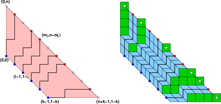
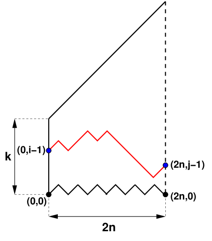
Recall that there is a local bijection between 3D-partitions, tilings of a plane (of a triangular lattice on a plane) by rhombi, and dimer configurations on the dual hexagonal lattice [6]. Another important local bijection is between lattice paths and rhombus tilings. It is illustrated on Fig.1.

The limit shape phenomenon is studied well in dimer models on hexagonal lattices and for corresponding tiling models in the case when the boundary of the domain consists of long pieces parallel to the axes of the triangular lattice. There are also some results for the case when the boundary is a fixed ”zig-zag” path. But in all cases the shape of the boundary is fixed.

The goal of this paper is to study the limit shapes when part of the boundary is a random variable. We call this “free boundary”. An example of a free boundary for a cut hexagon region is shown on Fig. 1. The end points of lattice paths on the Noth-East boundary are not fixed, which corresponds to variable configurations of boundary tiles.

In this paper we assume that configurations (tilings, 3D-partitions, paths) are distributed uniformly, or weighted with the probability

(0.1) $$Prob(S)\propto q^{|S|}$$

where $q$ is a real positive number, and $|S|$ is the volume under the height function corresponding to the configuration.

The computations are based on the Gessel-Vionnet formula for the number of lattice paths [3]. In the last section we compare our results with the analysis of limit shapes of height functions for dimer models based on the Burgers-Hopf equations [4].

In Section 1 we compute the boundary of the limit shape for cut hexagons (see Fig.1) of large size when the lattice paths are distributed as in (0.1). We assume that as the size of the cut hexagon increases, $q$ is approaching $1$ as $q=\exp(\varepsilon)$ where ${1\over\varepsilon}$ is proportional to the linear size of the system. In Section 2 we extend these results to the case when there are “frozen” triangles along the free boundary. In particular, when two frozen triangles are next to the ends of the free boundary, the problem includes the non-cut hexagon as a particular case Fig.5. In Section 3 we compare our results for the full hexagon with the paper [2] where they were derived originally. Finally Section 4 contains the comparison of our results with the derivation of the limit shape from the Hopf-Burgers equation [4]. In Section 5 we use a symmetry principle and the results obtained in previous sections to obtain the limit shape for the TSSCPP problem [7].

The work of N.R. was supported by Danish National Research Foundation through the Niels Bohr initiative, by the NSF grant DMS-0601912, and by DARPA. P.D.F. is supported in part by the ANR Grant GranMa, the ENIGMA research training network MRTN-CT-2004-5652, and the ESF program MISGAM.

1. Case of a cut hexagon

In this section we will focus on random tiling with weights (0.1). The goal is to find the asymptotic distribution of boundary positions of paths in the continuum limit i.e. when $k,n\to\infty$ and $q=\exp(\pm\varepsilon)\to 1$ such that $k\varepsilon\to\beta$ and $n\varepsilon\to\alpha$ are finite.

We will not give a rigorous proof of the existence of the limit shape, i.e. that the random boundary partition converges in probability to the limit shape function. We will give reasonable standard arguments, based on the variational principle, that it does, and compute the limit shape explicitly.

Figure 1. A typical tiling of the cut hexagon $n\times k\times n$, with free boundary conditions on the cut. We have represented the tiling on the square lattice. One keeps track of the two non-square tiles by drawing a segment in the middle. The segments form non-intersecting lattice paths, starting at points $(i-1,1-i)$, $i=1,2,...,k$ and ending on the cut $x+y=n$, at points $(m_{i},n-m_{i})$, $0\leq m_{i}\leq n+k-1$.

1.1. $q$-enumeration

Figure 2. The area under the path (green boxes) plus that in the top triangle (pink boxes) accounts for the partition function $q^{b(b-1)/2}{a\choose b}_{q}$ for lattice paths from $(0,0)$ to $(b,a-b)$, with a weight $q$ per box in the corresponding slice of plane partition.

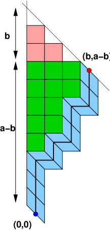
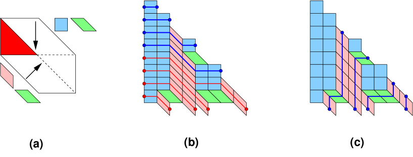
The generating function for the number of tilings viewed as plane partitions, with a weight $q$ per box (with green top) can be expressed as:

(1.1) $$Z_{k,n}({\mathbf{m}}|q)=\det_{1\leq i,j\leq k}q^{(m_{j}-i+1)(m_{j}-i)\over 2}{n\choose m_{j}-i+1}_{q}$$

where the $q$-binomial reads ${a\choose b}_{q}={[a]_{q}!\over[b]_{q}![a-b]_{q}!}$, and the $q$-factorial $[a]_{q}!=\prod_{i=1}^{a}(1-q^{i})$.

This formula is explained in Fig.2. The $q$-binomial ${a\choose b}_{q}$ enumerates the lattice paths from $(0,0)$ to $(b,a-b)$ with a weight $q^{A}$, where $A$ is the (discrete) area under the path, namely the number of unit squares in the domain delimited by the axes $x=0$, $y=a-b$ and the path. This gives the correct weight $q$ per box in the plane partition, within the slice containing the path, provided one adds up the contribution of the boxes in the domain delimited by $x=0$, $y=a-b$ and $x+y=a$ (pink boxes), with area ${b\choose 2}$, hence the additional prefactor $q^{m_{j}-i+1\choose 2}$.

The formula (1.1) factors out a Vandermonde type determinant and it has the following multiplicative form:

(1.2) $$Z_{k,n}({\mathbf{m}}|q)=q^{{k+1\choose 3}+{1\over 2}\sum_{i=1}^{k}m_{i}(m_{i}-2k+1)}\Delta(q^{\mathbf{m}})\,\prod_{i=1}^{k}{[n+k-i]_{q}!\over[m_{i}]_{q}![n+k-m_{i}-1]_{q}!}$$

where $\Delta(q^{\mathbf{m}})=\prod_{1\leq i,j\leq k}(q^{m_{i}}-q^{m_{j}})$.

The generating function is symmetric with respect to the mapping $q\to q^{-1}$

(1.3) $$Z_{k,n}({\mathbf{m}}|q)=q^{s_{k,n}}Z_{k,n}(\bar{{\mathbf{m}}}|q)$$

where $\bar{m}_{i}=n+k-1-m_{i}$, $s_{k,n}=-\frac{k^{3}-k}{2}-\frac{nk(n+k)}{2}+k(n+k-1)$.

1.2. The continuum limit

1.2.1.

Now we consider $\{{\mathbf{m}}\}$ as a random variable with

$$Prob(\{{\mathbf{m}}\})\propto Z_{k,n}({\mathbf{m}}|q)$$

and we will study this random variable in the limit when $q=e^{\pm\varepsilon}$, $\varepsilon\to+0$, $n,k\to\infty$, and $\alpha=n\varepsilon,\beta=k\varepsilon$ are fixed.

Let us start with the case $q=e^{-\varepsilon}$. The following results can be easily extended to $q=e^{\varepsilon}$ using the symmetry (1.3).

When $\varepsilon\to 0$ and $\mu=m\varepsilon$ is kept finite we have:

$${\rm Log}\,[m]_{q}!=\frac{1}{\varepsilon}\,\int_{0}^{\mu}{\rm Log}(1-e^{-x})dx+O(1)$$

Assume that as $\varepsilon\to 0$, the density

$$\mu(t)=\sum_{i=1}^{k}m_{i}\varepsilon\delta(t-i\varepsilon)$$

converges to the density corresponding to the continuous function $\mu(t)$ on the interval $[0,\beta]$. Then, the leading term of the asymptotic of the generating function (1.2) is given by

$$Z_{k,n}({\mathbf{m}}|q)=e^{-{1\over\varepsilon^{2}}S\{\mu\}+o({1\over\varepsilon})}$$

where

$$S\{\mu\} = \int_{0}^{\beta}{1\over 2}\mu(t)(\mu(t)-2\beta)+\int_{0}^{\beta}\left[\int_{0}^{\mu(t)}{\rm Log}(1-e^{-x})\,dx+\int_{0}^{\lambda+1-\mu(t)}\,{\rm Log}(1-e^{-x})\,dx\right]\,dt$$

$$-{1\over 2}\int_{0}^{\beta}\int_{0}^{\beta}{\rm Log}|e^{-\mu(s)}-e^{-\mu(t)}|\,ds\,dt+C({\alpha},\beta)$$

where $C({\alpha},\beta)$ reads:

$$C({\alpha},\beta)={1\over 6}-\int_{0}^{\beta}dx\int_{0}^{\alpha+\beta-x}\,{\rm Log}(1-e^{-y})\,dy$$

Assume that the function $\mu(t)$ is differentiable and consider the density $\rho(\mu)$:

$$\rho(\mu(t))={1\over\mu^{\prime}(t)},\ \ dt=\rho(\mu)d\mu$$

In terms of $\rho(\mu)$ the functional $S$ reads as

$$S[\rho] = \int_{0}^{\alpha+\beta}({1\over 2}\mu(\mu-2\beta)+L(\mu)+L(\alpha+\beta-\mu))\rho(\mu)d\mu$$

$$-{1\over 2}\mathchoice{{\vbox{\hbox{$\textstyle-$}}\kern-4.86108pt}}{{\vbox{\hbox{$\scriptstyle-$}}\kern-3.25pt}}{{\vbox{\hbox{$\scriptscriptstyle-$}}\kern-2.29166pt}}{{\vbox{\hbox{$\scriptscriptstyle-$}}\kern-1.875pt}}\!\int_{0}^{\alpha+\beta}\mathchoice{{\vbox{\hbox{$\textstyle-$}}\kern-4.86108pt}}{{\vbox{\hbox{$\scriptstyle-$}}\kern-3.25pt}}{{\vbox{\hbox{$\scriptscriptstyle-$}}\kern-2.29166pt}}{{\vbox{\hbox{$\scriptscriptstyle-$}}\kern-1.875pt}}\!\int_{0}^{\alpha+\beta}\ln|e^{-\mu}-e^{-\nu}|\rho(\mu)\rho(\nu)\,d\mu\,d\nu$$

where $L(x)=\int_{0}^{x}\ln(1-e^{-t})dt$.

In addition, since $\sum_{i=1}^{k}1=k$, we have

(1.4) $$\beta=\int_{0}^{\beta}dt=\int_{0}^{\alpha+\beta}\rho(\mu)d\mu$$

The functional $S[\rho]$ is convex and therefore has unique minimum.

It is easy to find the variation of this functional:

(1.5) $$\delta S[\rho]=\int_{0}^{\alpha+\beta}\left[{1\over 2}\mu(\mu-2\beta)+L(\mu)+L(\alpha+\beta-\mu)\right]\delta\rho(\mu)d\mu\\ -\mathchoice{{\vbox{\hbox{$\textstyle-$}}\kern-4.86108pt}}{{\vbox{\hbox{$\scriptstyle-$}}\kern-3.25pt}}{{\vbox{\hbox{$\scriptscriptstyle-$}}\kern-2.29166pt}}{{\vbox{\hbox{$\scriptscriptstyle-$}}\kern-1.875pt}}\!\int_{0}^{\alpha+\beta}\mathchoice{{\vbox{\hbox{$\textstyle-$}}\kern-4.86108pt}}{{\vbox{\hbox{$\scriptstyle-$}}\kern-3.25pt}}{{\vbox{\hbox{$\scriptscriptstyle-$}}\kern-2.29166pt}}{{\vbox{\hbox{$\scriptscriptstyle-$}}\kern-1.875pt}}\!\int_{0}^{\alpha+\beta}\ln|e^{-{\alpha}\mu}-e^{-{\alpha}\nu}|\rho(\nu)d\nu\delta\rho(\mu)d\mu$$

The second variation is positive definite:

$$\delta^{2}S[\rho]=-\mathchoice{{\vbox{\hbox{$\textstyle-$}}\kern-4.86108pt}}{{\vbox{\hbox{$\scriptstyle-$}}\kern-3.25pt}}{{\vbox{\hbox{$\scriptscriptstyle-$}}\kern-2.29166pt}}{{\vbox{\hbox{$\scriptscriptstyle-$}}\kern-1.875pt}}\!\int_{0}^{\alpha+\beta}\mathchoice{{\vbox{\hbox{$\textstyle-$}}\kern-4.86108pt}}{{\vbox{\hbox{$\scriptstyle-$}}\kern-3.25pt}}{{\vbox{\hbox{$\scriptscriptstyle-$}}\kern-2.29166pt}}{{\vbox{\hbox{$\scriptscriptstyle-$}}\kern-1.875pt}}\!\int_{0}^{\alpha+\beta}\ln|e^{-\mu}-e^{-\nu}|\delta\rho(\nu)\delta\rho(\mu)d\mu d\nu$$

Therefore the minimum of $S[\rho]$ is achieved at its critical point. Let us find the critical point of $S$ which satisfies the constraint (1.4). The convexity of $S$ guarantees its uniqueness.

The condition (1.4) implies the constraint on the variation of $\rho$:

$$\int_{0}^{\alpha+\beta}\delta\rho(\mu)\,d\mu=0$$

Taking it into account, we obtain the integral equation for critical points of $S[\rho]$:

$${1\over 2}\mu(\mu-2\beta)+L(\mu)+L(\alpha+\beta-\mu)-\mathchoice{{\vbox{\hbox{$\textstyle-$}}\kern-4.86108pt}}{{\vbox{\hbox{$\scriptstyle-$}}\kern-3.25pt}}{{\vbox{\hbox{$\scriptscriptstyle-$}}\kern-2.29166pt}}{{\vbox{\hbox{$\scriptscriptstyle-$}}\kern-1.875pt}}\!\int_{0}^{\alpha+\beta}\ln|e^{-\mu}-e^{-\nu}|\rho(\nu)\,d\nu=const$$

We want to solve it on the space of functions $\rho$ satisfying the constraint (1.4).

Differentiating this integral equation and taking into account (1.4) we arrive at

$$\ln({1-e^{-\mu}\over e^{-\mu}-e^{-\alpha-\beta}})=\mathchoice{{\vbox{\hbox{$\textstyle-$}}\kern-4.86108pt}}{{\vbox{\hbox{$\scriptstyle-$}}\kern-3.25pt}}{{\vbox{\hbox{$\scriptscriptstyle-$}}\kern-2.29166pt}}{{\vbox{\hbox{$\scriptscriptstyle-$}}\kern-1.875pt}}\!\int_{0}^{\alpha+\beta}{\rho(\nu)\,d(e^{-\nu})\over e^{-\mu}-e^{-\nu}}$$

After changing variables to $u=e^{-\nu}$ and $L=e^{-\alpha-\beta}$ the equation for the density $\sigma(u)=\rho(\nu)$ becomes

(1.6) $$\ln({z-L\over 1-z})=\mathchoice{{\vbox{\hbox{$\textstyle-$}}\kern-4.86108pt}}{{\vbox{\hbox{$\scriptstyle-$}}\kern-3.25pt}}{{\vbox{\hbox{$\scriptscriptstyle-$}}\kern-2.29166pt}}{{\vbox{\hbox{$\scriptscriptstyle-$}}\kern-1.875pt}}\!\int_{L}^{1}{\sigma(u)\,du\over z-u}$$

where the function $\sigma$ satisfies the condition

(1.7) $$\int_{L}^{1}{\sigma(u)du\over u}=\beta$$

1.2.2.

Now let us solve (1.6) on the surface of the constraint (1.7) explicitly.

Proposition 1.1.

The unique solution to (1.6) subject to the constraint (1.7) is

(1.8) $$\rho(\mu)=\sigma(e^{-\mu})={2\over\pi}{\rm Arctan}\left(e^{-\mu}\sqrt{{\rm sinh}\,{(\mu-A)\over 2}\,{\rm sinh}\,{(B-\mu)\over 2}\over{\rm sinh}\,{A\over 2}\,{\rm sinh}\,{B\over 2}}\right)$$

where

$$e^{-B} = e^{-{{\alpha}+\beta\over 2}}\left({\rm cosh}\,{{\alpha}+\beta\over 2}-\sqrt{{\rm sinh}\,{\beta\over 2}\,{\rm sinh}\,{2{\alpha}+\beta\over 2}}\right)$$

(1.9) $$e^{-A} = e^{-{{\alpha}+\beta\over 2}}\left({\rm cosh}\,{{\alpha}+\beta\over 2}+\sqrt{{\rm sinh}\,{\beta\over 2}\,{\rm sinh}\,{2{\alpha}+\beta\over 2}}\right)$$

Proof.

Assume the support of $\sigma$ is the interval $[a,b]\subset[L,1]$ and consider the function

$$F(z)=\int_{a}^{b}{\sigma(u)\,du\over z-u}$$

on the complex plane with the branch cut along $[a,b]$. It is a meromorphic function whose boundary values at the interval $[a,b]$ satisfy the relation

$$2\ln({z-L\over 1-z})=F(z+i0)+F(z-i0)$$

and $F(z)=O({1\over z})$ as $|z|\to\infty$.

To solve this equation explicitly consider the function $G(z)={1\over\sqrt{(z-a)(z-b)}}F(z)$. It is a meromorphic function on the complex plane with the branch cut along $[a,b]$. But now at the branch cut we have

$$G(z+i0)-G(z-i0)=2{1\over\sqrt{(z-a)(z-b)}}\ln({z-L\over 1-z})$$

and $G(z)=O({1\over z^{2}})$ as $|z|\to\infty$. From here we obtain:

(1.10) $$F(z)={1\over\pi}\sqrt{(z-a)(z-b)}\int_{a}^{b}{1\over\sqrt{(u-a)(b-u)}}\,{\rm Log}{u-L\over 1-u}\,{du\over z-u}\,$$

As $|z|\to\infty$ this function behave as

$$F(z)={1\over\pi}\int_{L}^{1}{1\over\sqrt{(u-a)(b-u)}}\,{\rm Log}{u-L\over 1-u}\,du\,+O({1\over z})$$

This gives the first equation for $a,b$:

$$\int_{L}^{1}{1\over\sqrt{(u-a)(b-u)}}\,{\rm Log}{u-L\over 1-u}\,du=0$$

It is easy to see that the integral vanishes when $a+b=1+L$.

Changing the integration variable in (1.10) $u=(b-a)s+a$ and taking into account the relation between $a$ and $b$ we obtain the following integral formula for $F(z)$:

$$F(z)={1\over\pi}\sqrt{(z-a)(z-b)}\int_{0}^{1}{1\over\sqrt{s(1-s)}}\,{\rm Log}{s+M\over 1+M-s}\,{ds\over t-s}\,$$

where $t={z-a\over b-a}$, and $M={a-L\over 1+L-2a}$.

This integral can be computed explicitly using

$$\int_{0}^{1}{1\over(w-u)(\beta+u)\sqrt{u(1-u)}}du={\pi\over\beta+w}\left({1\over\sqrt{\beta(\beta+1)}}+{1\over\sqrt{w(w-1)}}\right)$$

and we obtain:

$$F(z)=\ln{z-L\over 1-z}+2i{\rm Arctan}\sqrt{(z-a)(b-z)\over(a-L)(1-a)}$$

The second equation determining $a$ and $b$ is the normalization (1.4). It gives $F(0)=-\beta$ and therefore:

$$\sqrt{(1-a)(1-b)\over ab}={\rm tanh}{\alpha\over 2}$$

This gives $a$ and $b$:

$$a = e^{-{{\alpha}+\beta\over 2}}\left({\rm cosh}\,{{\alpha}+\beta\over 2}-\sqrt{{\rm sinh}\,{\beta\over 2}\,{\rm sinh}\,{2{\alpha}+\beta\over 2}}\right)$$

(1.11) $$b = e^{-{{\alpha}+\beta\over 2}}\left({\rm cosh}\,{{\alpha}+\beta\over 2}+\sqrt{{\rm sinh}\,{\beta\over 2}\,{\rm sinh}\,{2{\alpha}+\beta\over 2}}\right)$$

The density $\rho(\mu)$ can be easily derived from $F(z)$ as $\rho(\mu)=ImF(e^{-\mu})$ when $\mu\in[B,A]$, and $B=-{\rm Log}\,b$, $A=-{\rm Log}\,a$:

(1.12) $$\rho(\mu)=\sigma(e^{-\mu})={2\over\pi}{\rm Arctan}\left(e^{-\mu}\sqrt{{\rm sinh}\,{(\mu-A)\over 2}\,{\rm sinh}\,{(B-\mu)\over 2}\over{\rm sinh}\,{A\over 2}\,{\rm sinh}\,{B\over 2}}\right)$$

∎

Because the solution $\rho$ described above is a local minimum of the convex functional $S$. it is also a global minimum.

The density $\rho(\mu)$ is plotted on Fig.3 for $\lambda=1/2,1,2,5$ and $\beta=0,1/2,1,2,5$. Here $\lambda=\alpha/\beta$.

Figure 3. Distribution of endpoints for $\lambda={\alpha}/\beta=1/2,1,2,5$ and $\beta=0,1/2,1,2,5$ (from right to left, in each plot).

1.2.3.

The limit when ${\alpha}=\beta\lambda$ and ${\alpha}\to 0$ while $\lambda$ is fixed correspond to the limit shape for uniformly weighted lattice paths, i.e to $q=1$.

In this limit $A=\beta A_{0}$, $B=\beta B_{0}$ where

(1.13) $$B_{0}(\lambda) = {1+\lambda\over 2}-\sqrt{{1\over 2}(1+{\lambda\over 2})}$$

(1.14) $$A_{0}(\lambda) = {1+\lambda\over 2}+\sqrt{{1\over 2}(1+{\lambda\over 2})}$$

The density of endpoints on the free boundary converges to

(1.15) $$\rho(t)={2\over\pi}{\rm Arctan}\left(\sqrt{{(t-A_{0})(B_{0}-t)\over A_{0}B_{0}}}\right)={2\over\pi}{\rm Arctan}\left({\sqrt{2\lambda+1-4(t-{\lambda+1\over 2})^{2}}\over\lambda}\right)$$

here $t=\mu/\beta$.

1.2.4.

Another interesting limit is when ${\alpha}\to\infty$ while $\beta$ is fixed. In this case $\rho$ is given by the same formula as before but for the boundary points we have:

$$e^{-B}\to{1\over 2}(1-\sqrt{1-e^{-\beta}})$$

$$e^{-A}\to{1\over 2}(1+\sqrt{1-e^{-\beta}})$$

Note finally that all the above is valid for ${\alpha}<0$ as well. The transformation ${\alpha}\to-{\alpha}$ amounts to reflecting the plane partition w.r.t. the axis $y=x$ as in (1.3).

2. Case of a cut hexagon with forbidden intervals along the free boundary

In the previous section we studied boundary partition for the distribution $q^{|S|}$. From now on we will consider the uniform distribution. All results can be easily generalized to $q\neq 1$ but we will not do it here.

2.1. Enumeration

Figure 4. The domain to be tiled is a half-hexagon $n\times k\times n$ with the fixed interval of $m$ square tiles along the boundary.

We consider the domain of Fig.4, made of a cut hexagon $n\times k\times n$ with a fixed interval of square tiles along the boundary. The effect of these tiles is that lattice paths are forbidden to have endpoints along a segment of the form $\{(i,n-i),\ i=n_{1},n_{1}+1,\ldots n_{1}+m-1\}$, while $n_{1}+m+n_{2}=n+k$.

It is clear that the counting formula is the same Gessel-Viennot formula as in the previous problem with $q=1$:

(2.1) $$Z_{k,n}({\mathbf{m}})=\det_{1\leq i,j\leq k}{n\choose m_{j}-i+1}$$

It can be written in the multiplicative form:

(2.2) $$Z_{k,n}({\mathbf{m}})=\prod_{1\leq i,j\leq k}(m_{i}-m_{j})\,\prod_{i=1}^{k}{[n+k-i]!\over[m_{i}]![n+k-m_{i}-1]!}$$

The difference with the previous case is that positions of end points of lattice paths $m_{i}$ now can only be in $[0,n+k-1]\setminus[n_{1},n_{1}+m-1]=[0,n_{1}-1]\cup[n_{1}+m,n+k-1]$. The interval $[n_{1},n_{1}+m-1]$ is forbidden.

2.2. Large size asymptotics

Here we will study the distribution of endpoints in the limit when $k\to\infty$ and $n=\lambda k$, $n_{1}=\lambda_{1}k$, $n_{1}+m=\lambda_{2}k$, $m_{i}=\mu_{i}k$, for some finite $\lambda,\lambda_{1}$, and $\lambda_{2}$.

The large $k$ asymptotics of the number of lattice paths with endpoints fixed outside of the forbidden intervals is given by the action function

(2.4) $$S_{\lambda}[\rho] = \int_{0}^{\lambda+1}({1\over 2}\mu(\mu-2\lambda)+L_{0}(\mu)+L_{0}(\lambda+1-\mu))\rho(\mu)d\mu$$

$$-{1\over 2}\mathchoice{{\vbox{\hbox{$\textstyle-$}}\kern-4.86108pt}}{{\vbox{\hbox{$\scriptstyle-$}}\kern-3.25pt}}{{\vbox{\hbox{$\scriptscriptstyle-$}}\kern-2.29166pt}}{{\vbox{\hbox{$\scriptscriptstyle-$}}\kern-1.875pt}}\!\int_{0}^{\lambda+1}\mathchoice{{\vbox{\hbox{$\textstyle-$}}\kern-4.86108pt}}{{\vbox{\hbox{$\scriptstyle-$}}\kern-3.25pt}}{{\vbox{\hbox{$\scriptscriptstyle-$}}\kern-2.29166pt}}{{\vbox{\hbox{$\scriptscriptstyle-$}}\kern-1.875pt}}\!\int_{0}^{\lambda+1}\ln|\mu-\nu|\rho(\mu)\rho(\nu)\,d\mu\,d\nu$$

where $L_{0}(x)=x{\rm Log}(x)-x$.

This is a convex functional. The same arguments as in the previous section shows that its extremum is the unique minimum. Assume that the forbidden segment $[\lambda_{1},\lambda_{2}]$ is in a generic position which means that the region where the density is not constant (not $0$ or $1$) consists of two segments $T=[a,b]\cup[c,d]$, such that $0<a<b<\lambda_{1}<\lambda_{2}<c<d<\lambda+1$. The density is constant outside of $T$:

$$\rho(\mu)=0,\ \ \mu\in[0,a]\cup[d,\lambda+1],\ \ \rho(\mu)=1,\ \ \mu\in[b,\lambda_{1}]\cup[\lambda_{2},c]$$

The density $\rho(\mu)$ which minimizes $S[\rho]$ satisfies the integral equation

(2.5) $${\rm Log}{u(b-u)(u-\lambda_{2})\over(\lambda+1-u)(\lambda_{1}-u)(u-c)}=\mathchoice{{\vbox{\hbox{$\textstyle-$}}\kern-4.86108pt}}{{\vbox{\hbox{$\scriptstyle-$}}\kern-3.25pt}}{{\vbox{\hbox{$\scriptscriptstyle-$}}\kern-2.29166pt}}{{\vbox{\hbox{$\scriptscriptstyle-$}}\kern-1.875pt}}\!\int_{T}{\rho(\mu)d\mu\over u-\mu}$$

$u\in T$ with the additional constraint:

$$\int_{T}\rho(u)du+(\lambda_{1}-b)+(c-\lambda_{2})=1$$

The solution to the integral equation (2.5) with the additional constraints can be obtained in the similar way as before by converting the integral equation to the problem of finding the holomorphic function with given boundary values. For the resolvent

$$F(z)=\int_{T}{\rho(u)du\over z-u}$$

we obtain the following integral expression

(2.7) $$F(z) = {1\over\pi}\sqrt{(z-a)(z-b)(z-c)(z-d)}$$

$$\times\,\int_{T}{du\over\sqrt{(b-u)(u-a)(c-u)(d-u)}}\,{1\over z-u}\,{\rm Log}\,{u(b-u)(u-\lambda_{2})\over(\lambda+1-u)(\lambda_{1}-u)(u-c)}$$

The end points $a,b,c,d$ are determined by the asymptotic behavior $F(z)=(1+\lambda_{2}-\lambda_{1}+b-c)/z+O(1/z^{2})$ at large $z$. Indeed, if there were no conditions on $a,b,c,d$ the resolvent would behave as $z^{2}$ for large $z$. Vanishing coefficients in $z^{2}$, $z$, $z^{0}$, and fixing the coefficient in $z^{-1}$ give four equations. If the parameters $\lambda,\lambda_{1},\lambda_{2}$ are in generic position, these equations have a real solution, which gives the desired values of $a,b,c,d$ as functions of $\lambda,\lambda_{1},\lambda_{2}$.

The density is given by the imaginary part of the boundary value for the resolvent on $T$:

(2.8) $$\rho(z)={\rm Im}\,F(z+i0)/\pi,\ \ z\in T$$

For sufficiently small values of $\lambda_{1}$ the interval $[a,b]$ may shrink to a point. The same can happen with the interval $[c,d]$ for sufficiently large values of $\lambda_{2}$. Both intervals shrink to a point when $\lambda_{2}-\lambda_{1}=\lambda$. It is impossible to have $\lambda_{2}-\lambda_{1}>\lambda$ because in this case the number of lattice paths incoming to the region would be greater then the number of paths outgoing from it.

2.3. Case of many forbidden intervals

This is a straightforward generalization of the previous case to a succession of forbidden intervals along the free boundary.

The number of lattice paths is still given by the formula (2.1). The only difference is that all $m_{i}$ should be outside of the forbidden intervals.

Denote by $[{\alpha}_{i},\beta_{i}]$ the forbidden intervals $i=1,\dots,l$. The density of the outgoing paths is supported on $\cup_{i=1}^{l+1}[\beta_{i-1},{\alpha}_{i}]$ where $\beta_{0}=0$ and ${\alpha}_{l+1}=\lambda+1$. Let us say ${\alpha}_{i},\beta_{i}$ are generic when the minimizer of the rate functional $S[\rho]$ is constant on the following intervals:

$$\rho(u)=1,u\in\cup_{i=2}^{l+1}[\beta_{i-1},a_{i}]\cup[b_{i-1},{\alpha}_{i-1}],\ \ \rho(u)=0,u\in[0,a_{1}]\cup[b_{l+1},\lambda+1]$$

The integral equation for the minimizer is

$${\rm Log}\left({\mu\over\lambda+1-\mu}\prod_{i=2}^{l+1}{(\mu-b_{i-1})(\mu-\beta_{i-1})\over({\alpha}_{i-1}-\mu)(a_{i}-\mu)}\right)=\mathchoice{{\vbox{\hbox{$\textstyle-$}}\kern-4.86108pt}}{{\vbox{\hbox{$\scriptstyle-$}}\kern-3.25pt}}{{\vbox{\hbox{$\scriptscriptstyle-$}}\kern-2.29166pt}}{{\vbox{\hbox{$\scriptscriptstyle-$}}\kern-1.875pt}}\!\int_{T}dw{\rho(w)\over\mu-w}$$

where $T=\cup_{i}[a_{i},b_{i}]$.

The minimizer satisfies the constraint (the number of incoming paths is equal to the number of outgoing paths):

$$\int_{T}\rho(u)du+\sum_{i=2}^{l+1}(a_{i}-\beta_{i-1})+\sum_{i=1}^{l}({\alpha}_{i}-b_{i})=1$$

The solution to this integral equation is given by the the resolvent function

$$F(z)={1\over\pi}\int_{T}du\prod_{i}{\sqrt{(z-a_{i})(z-b_{i})}\over\sqrt{(b_{i}-u)(u-a_{i})}}\,{1\over z-u}\,{\rm Log}\,{u\over\lambda+1-u}\prod_{i}{(u-b_{i-1})(u-\beta_{i-1})\over({\alpha}_{i-1}-u)(a_{i}-u)}$$

as usual:

$$\rho(z)={\rm Im}\,F(z+i0)/\pi,\ \ z\in T$$

2.4. The case of forbidden and fully packed intervals

2.4.1.

Forbidden intervals are just one way to partially enforce boundary conditions along segments of the free boundary, where one imposes $\rho=0$. Another special case is that of fully packed intervals, along which every point is an end point of a lattice path, hence $\rho=1$ is imposed.

We cannot enforce a given type of tiles along a fully packed interval. However the geometry of tiles is such that each fully packed interval has a sequence of non-square tiles which start with horizontally tilted tiles at the top and then horizontal tiles turn at some point into vertical non-square tiles. The position of the turning point is random: it is not fixed by the requirement that the interval is fully packed.

The counting formula for the number of lattice paths is the same as before and we can compute the limit density of end points of lattice paths along the free part of the boundary similarly to the case when we have only forbidden intervals.

2.4.2.

The problem of finding the limit density for one fully packed interval is very similar to the problem for one forbidden interval. Lattice paths come to the fully packed interval horizontally at the upper part of the interval and vertically at the lower part of the interval. Such a configuration induces forbidden intervals at both ends of the fully packed interval. Let $l_{1}$ and $l_{2}$ be end-points of the fully packed interval. In the limit when $k,n,l_{1},l_{2}\to\infty$ such that $\lambda=n/k,\lambda_{i}=l_{i}/k$ are finite the resulting density of lattice paths has the following structure

$$\rho(\mu)=0,\ \ \mu\in[0,a]\cup[d,\lambda+1],\ \ \rho(\mu)=0,\ \ \mu\in[b,\lambda_{1}]\cup[\lambda_{2},c]$$

Here $0<a<b<\lambda_{1}<\lambda_{2}<c<d<1+\lambda$, $\rho(\mu)=1$ when $\mu\in[\lambda_{1},\lambda_{2}]$ and $\rho(\mu)$ is a smooth functions when $\mu\in T=[a,b]\cup[c,d]$. It satisfies the constraint

$$\int_{T}\rho(\mu)d\mu+(\lambda_{2}-\lambda_{1})=1$$

The limit density on $T$ is determined by the variational problem similar to the one described above and the solution is given by the resolvent function eq. (2.7). The density is equal to the imaginary part of the resolvent on $T$ eq. (2.8). The endpoints $a,b,c,d$ are determined by the condition $F(z)=(1+\lambda_{1}-\lambda_{2})/z+O(1/z^{2})$.

When a fully packed interval is near any boundary of the whole interval $[0,\lambda+1]$, the lattice paths form a “fully packed region” along the corresponding side of the cut hexagon. In this case the problem of finding the limit density of paths is equivalent to the problem for a cut hexagon of smaller size.

2.4.3.

The generic case of several fully packed and forbidden intervals corresponds to an alternance of the intervals, apart from one-another. All other situations are degenerations of this one.

The equation for the density in this case is similar to the case when we have several forbidden intervals. Let $[\alpha_{i},\beta_{i}]$ be forbidden intervals and $[\lambda_{i},\nu_{i}]$ be fully packed intervals. Assume that $\beta_{i}<\lambda_{i}$ for all $i=1,\dots,n$. When the boundaries of intervals are in generic position the density will vary smoothly in intervals $[a_{i},b_{i}]$, $[c_{i},d_{i}]$, $i=1,\dots,n$ where $\dots<b_{i}<\alpha_{i}<\beta_{i}<c_{i}<d_{i}<\lambda_{i}<\mu_{i}<a_{i+1}<b_{i+1}<\dots$, and $d_{n}<\lambda+1$. The density is $1$ in fully packed intervals and $0$ in the forbidden intervals. In addition in is $1$ in intervals $[b_{i},\alpha_{i}]$, $[\beta_{i},c_{i}]$, and it is $0$ in the intervals $[d_{i},\lambda_{i}]$, $[\nu_{i},a_{i+1}]$, $[0,a_{1}]$, and $[d_{n},\lambda+1]$.

The density function satisfies the constraint:

$$\sum_{i=1}^{n}\int_{T}\rho(\mu)d\mu+\sum_{i=1}^{n}((\alpha_{i}-b_{i})+(c_{i}-\beta_{i})+(\nu_{i}-\lambda_{i}))=1$$

where $T=\cup_{i=1}^{n}[a_{i},b_{i}]\cup[c_{i},d_{i}]$ The solution to the integral equation for the minimizer is given by the resolvent:

$$F(z) = {1\over\pi}\int_{T}du\prod_{i=1}^{n}{\sqrt{(z-a_{i})(z-b_{i})(z-c_{i})(z-d_{i})}\over\sqrt{(b_{i}-u)(u-a_{i})(u-c_{i})(u-d_{i})}}$$

$$\ \ \ \ \ \ \times\,{1\over z-u}\,{\rm Log}\,{u\over\lambda+1-u}\prod_{i=1}^{n}{(u-b_{i})(u-\beta_{i})(u-\lambda_{i})\over(u-\alpha_{i})(u-c_{i})(u-\mu_{i})}$$

The constraint on the density is equivalent to the following condition on the asymptotics of $F(z)$:

$$F(z)=(1-\sum_{i=1}^{n}((\alpha_{i}-b_{i})+(c_{i}-\beta_{i})+(\nu_{i}-\lambda_{i})))/z+O(1/z^{2})$$

which gives equations defining $a_{i},b_{i},c_{i},d_{i}$. The density is given by the imaginary part of $F(z)$ on $T$ as in eq. (2.8).

2.5. Case of two forbidden intervals at the corners

Here we consider the case of two forbidden intervals that touch respectively the top and the bottom of the free boundary. We will see that in this case the limit density can be computed explicitly in terms elementary functions.

Assume that the upper interval has length $m$ and that the lower one is of length $p$. Now the values $m_{i}\in[0,m]$ and $m_{i}\in[n+k-p-1,n+k-1]$ are forbidden, and hence the allowed range for endpoints of lattice paths is $[m+1,n+k-p-2]$.

Now we will take $k\to\infty$ such that $n=\lambda k$, $m=\nu k$, $n+k-p=\theta k$, which finite $\lambda,\nu,\theta$ and will compute the minimizer of the rate function $S[\rho]$.

2.5.1.

For generic $\nu,\theta$ the minimizer of the rate functional is not constant on the interval $[a,b]$ with $\nu<a<b<\theta$, and

$$\rho(u)=1,u\in[\nu,a]\cup[b,\theta]$$

It satisfies the integral equation

(2.9) $${\rm Log}\left({\mu(\mu-a)(\theta-\mu)\over(\lambda+1-\mu)(\mu-\nu)(b-\mu)}\right)=\mathchoice{{\vbox{\hbox{$\textstyle-$}}\kern-4.86108pt}}{{\vbox{\hbox{$\scriptstyle-$}}\kern-3.25pt}}{{\vbox{\hbox{$\scriptscriptstyle-$}}\kern-2.29166pt}}{{\vbox{\hbox{$\scriptscriptstyle-$}}\kern-1.875pt}}\!\int_{a}^{b}dw{\rho(w)\over\mu-w}$$

and the constraint

(2.10) $$\int_{a}^{b}\rho(w)dw=1-(a-\nu)-(\theta-b)$$

In this case the integrals can be computed explicitly.

Proposition 2.1.

The density is given by

$$\rho(z)=1+{2\over\pi}\left({\rm Arctan}\,\sqrt{b-z\over z-a}\sqrt{a-\nu\over b-\nu}-{\rm Arctan}\,\sqrt{b-z\over z-a}\sqrt{a\over b}\right.$$

$$\qquad\qquad\left.+{\rm Arctan}\,\sqrt{z-a\over b-z}\sqrt{\theta-b\over\theta-a}-{\rm Arctan}\,\sqrt{z-a\over b-z}\sqrt{\lambda+1-b\over\lambda+1-a}\,\right)$$

with

(2.13) $$a={1\over 4\lambda^{2}}(U(\lambda,\nu,\theta)-\sqrt{V(\lambda,\nu,\theta)})\qquad b={1\over 4\lambda^{2}}(U(\lambda,\nu,\theta)+\sqrt{V(\lambda,\nu,\theta)})$$

where $U$ and $V$ are the following polynomials:

$$U(\lambda,\nu,\theta) = (\nu+\theta)\Big{(}1-(\nu-\theta)^{2}\Big{)}-(\lambda+1)\Big{(}(1-\nu-\theta)(1+2\lambda+\nu+\theta)+4\nu\theta\Big{)}$$

$$V(\lambda,\nu,\theta) = (1-\nu-\theta)(1-\nu+\theta)(1+\nu-\theta)$$

$$\qquad\times(1+\nu-\theta+2\lambda)(1-\nu+\theta+2\lambda)(1-\nu-\theta+2\lambda)$$

Proof.

The resolvent for (2.9) is given by the integral

$$F(z)={\sqrt{w(w-1)}\over\pi}\int_{0}^{1}{dv\over\sqrt{v(1-v)}}\,{1\over w-v}\,{\rm Log}\left({(\beta+v)v(\eta-v)\over(\gamma-v)(\delta+v)(1-v)}\right)$$

where $w={z-a\over b-a}$ and

(2.14) $$\beta={a\over b-a},\quad\gamma={\lambda+1-a\over b-a},\quad\delta={a-\nu\over b-a},\quad\eta={\theta-a\over b-a}$$

The normalization condition (2.10) for the density is equivalent to large $z$ asymptotic behavior for the resolvent $F(z)={1+b-a+\nu-\theta\over z}+O({1\over z^{2}})$. Vanishing of the coefficient in $z$ and the constant term of this asymptotic amounts to:

(2.15) $$0=\int_{0}^{1}{dv\over\sqrt{v(1-v)}}\,{\rm Log}\left({(\beta+v)v(\eta-v)\over(\gamma-v)(\delta+v)(1-v)}\right)$$

(2.16) $$1-(\delta+\eta)(b-a)={b-a\over\pi}\int_{0}^{1}{dv\over\sqrt{v(1-v)}}\,v\,{\rm Log}\left({(\beta+v)v(\eta-v)\over(\gamma-v)(\delta+v)(1-v)}\right)$$

Using identities

(2.17) $$\int_{0}^{1}{1\over\sqrt{u(1-u)}}{\rm Log}(\beta+u)du=2\pi{\rm Log}\left({\sqrt{\beta}+\sqrt{\beta+1}\over 2}\right)$$

(2.18) $$\int_{0}^{1}{1\over\sqrt{u(1-u)}}u{\rm Log}(\beta+u)du={\pi\over 2}\left((\sqrt{\beta}-\sqrt{\beta+1})^{2}+2{\rm Log}\left({\sqrt{\beta}+\sqrt{\beta+1}\over 2}\right)\right)$$

we obtain equations

$$0 = \Big{(}\sqrt{\beta}+\sqrt{\beta+1}\Big{)}\Big{(}\sqrt{\eta}+\sqrt{\eta-1}\Big{)}-\Big{(}\sqrt{\gamma}+\sqrt{\gamma-1}\Big{)}\Big{(}\sqrt{\delta}+\sqrt{\delta+1}\Big{)}$$

$$1 = {b-a\over 2}\Big{\{}2(\delta+\eta+1)+(\sqrt{\beta+1}-\sqrt{\beta})^{2}+(\sqrt{\gamma-1}-\sqrt{\gamma})^{2}$$

$$\qquad\qquad\qquad\qquad\qquad-(\sqrt{\delta+1}-\sqrt{\delta})^{2}-(\sqrt{\eta-1}-\sqrt{\eta})^{2}\Big{\}}$$

The integral defining the resolvent can be evaluated explicitly using the following idenity

$${\sqrt{w(w-1)}\over\pi}\int_{0}^{1}{dv\over\sqrt{v(1-v)}}\,{1\over w-v}\,{\rm Log}\,{A+v\over B+v}=$$

(2.19) $$\qquad\qquad{\rm Log}\,{A+w\over B+w}+2i\left({\rm Arctan}\,\sqrt{1-w\over w}\sqrt{B\over 1+B}-{\rm Arctan}\,\sqrt{1-w\over w}\sqrt{A\over 1+A}\right)$$

It results in the formula:

$$F(z)={\rm Log}\left({(\beta+w)w(\eta-w)\over(\gamma-w)(\delta+w)(1-w)}\right)+2i\left({\rm Arctan}\,\sqrt{1-w\over w}\sqrt{\delta\over 1+\delta}\right.$$

$$\left.-{\rm Arctan}\,\sqrt{1-w\over w}\sqrt{\beta\over 1+\beta}+{\rm Arctan}\,\sqrt{w\over 1-w}\sqrt{\eta-1\over\eta}-{\rm Arctan}\,\sqrt{w\over 1-w}\sqrt{\gamma-1\over\gamma}\,\right)$$

Using this expression for the resolvent, vanishing conditions (2.15)(2.16) can be written as:

(2.20) $$a={1\over 4\lambda^{2}}(U(\lambda,\nu,\theta)-\sqrt{V(\lambda,\nu,\theta)})\qquad b={1\over 4\lambda^{2}}(U(\lambda,\nu,\theta)+\sqrt{V(\lambda,\nu,\theta)})$$

where $U$ and $V$ are the following polynomials:

$$U(\lambda,\nu,\theta) = (\nu+\theta)\Big{(}1-(\nu-\theta)^{2}\Big{)}-(\lambda+1)\Big{(}(1-\nu-\theta)(1+2\lambda+\nu+\theta)+4\nu\theta\Big{)}$$

$$V(\lambda,\nu,\theta) = (1-\nu-\theta)(1-\nu+\theta)(1+\nu-\theta)$$

$$\qquad\times(1+\nu-\theta+2\lambda)(1-\nu+\theta+2\lambda)(1-\nu-\theta+2\lambda)$$

From the formula for the resolvent we can compute the density $z\in[a,b]$:

(2.21) $$\rho(z)={\rm Im}\,F(z+i0)/\pi=1+{2\over\pi}\left({\rm Arctan}\,\sqrt{b-z\over z-a}\sqrt{a-\nu\over b-\nu}-{\rm Arctan}\,\sqrt{b-z\over z-a}\sqrt{a\over b}\right.$$

$$\qquad\qquad\left.+{\rm Arctan}\,\sqrt{z-a\over b-z}\sqrt{\theta-b\over\theta-a}-{\rm Arctan}\,\sqrt{z-a\over b-z}\sqrt{\lambda+1-b\over\lambda+1-a}\,\right)$$

valid for $\nu,\theta$ satisfying $\nu<a<b<\theta$. Note that $\rho(a)=\rho(b)=1$. ∎

2.5.2.

When the size of any of the forbidden intervals in sufficiently small, it merges with the nearest end of the interval $[a,b]$. For example when

$$\theta=\theta_{c}={1\over 3}\Big{(}1+\lambda+\nu+\sqrt{3(1+2\lambda)+(1+\lambda-2\nu)^{2}}\Big{)}$$

the lower forbidden interval connects to $[a,b]$: $b=\theta_{c}$. When $\theta<\theta_{c}$ they remain connected, i.e. in this case we still have $b=\theta$.

The same holds for the upper forbidden interval, in which case when

$$\nu=\nu_{c}={1\over 3}\Big{(}1+\lambda+\theta-\sqrt{3(1+2\lambda)+(1+\lambda-2\theta)^{2}}\Big{)}$$

the upper forbidden interval connects with $[a,b]$, $a=\nu_{c}$ and they stay connected for $\nu<\nu_{c}$.

The assumption $\nu<a<b<\theta$ which we used in the previous section holds when $\theta<\theta_{c}$ and $\nu>\nu_{c}$.

In $\theta\geq\theta_{c}$ and $\nu>\nu_{c}$ the region where $\rho(u)$ is not constant becomes $[a,\theta_{c}]$ with

$$a={b(1+\lambda+\nu-b)^{2}\over\lambda^{2}}$$

The density in this case can be obtained from (2.1) by setting $b,\theta\to\theta_{c}$. The result is

(2.23) $$\rho(z)={2\over\pi}\left({\rm Arctan}\,\sqrt{\theta_{c}-z\over z-a}\sqrt{a-\nu\over\theta_{c}-\nu}-\right.\\ \left.{\rm Arctan}\,\sqrt{\theta_{c}-z\over z-a}\sqrt{a\over\theta_{c}}-{\rm Arctan}\,\sqrt{z-a\over\theta_{c}-z}\sqrt{\lambda+1-\theta_{c}\over\lambda+1-a}\,\right)$$

It is easy to see that now the density satisfies $\rho(a)=1,\rho(b)=0$.

The formula above is valid as long as $\nu>\nu^{\prime}_{c}$, namely where

$$\nu_{c}^{\prime}=\nu_{c}|_{\theta=\theta_{c}}={1+\lambda-\sqrt{1+2\lambda}\over 2}$$

When $\nu\leq\nu^{\prime}_{c}$ the upper forbidden interval connects to the interval $[a,b]$. In this case

$$a={1+\lambda-\sqrt{1+2\lambda}\over 2},\ \ b={1+\lambda+\sqrt{1+2\lambda}\over 2}$$

The density inside of $[a,b]$ can be obtained from (2.23) by taking $a,\nu\to\nu^{\prime}_{c}$. The result is

$$\rho(z)=\sqrt{{(\theta^{\prime}_{c}-z)(z-\nu^{\prime}_{c})\over\theta^{\prime}_{c}\nu^{\prime}_{c}}}$$

which agrees with (1.15).

Remark 2.2.

The transition from free to trapped paths is similar to that found by Douglas and Kazakov in QCD.

2.5.3.

When $\theta+\nu=1$ the interval $[a,b]$ collapses into a point.

3. Case of the full hexagon

Figure 5. We decompose the hexagon $1\times\theta\times\lambda$ into two cut hexagons with one side equal to $1$, and with possible triangular holes at corners. Three cases must be considered.

In this section we will reproduce the results of [2] for the limit shape of the hexagon tiling and will prepare the ground for the next section where we will use the symmetries of regions to find the limit density at free boundaries for more complicated regions then in previous sections.

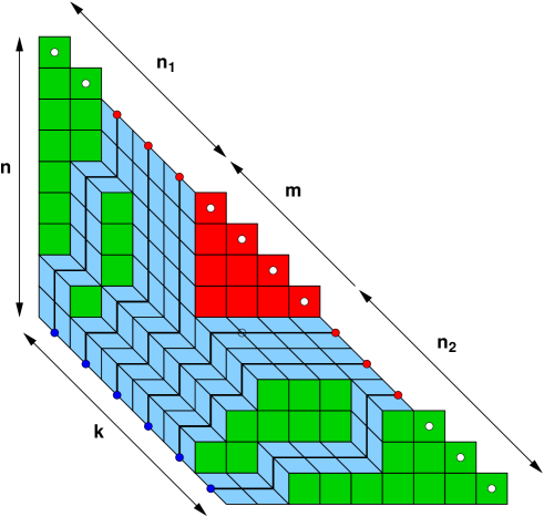
Cut the hexagon as it is illustrated in Fig.5 into two cut hexagons. In this section we will study the limit density of tiles by studying the the limit density of lattice path points intersecting an arbitrary cut (dashed line) which is parallel to one side of the hexagon . We assume that the hexagon has size $k\times n\times p$, and that the cut is at a distance $m$ from the edge of length $k$. Our goal to pass to the limit $k\to\infty$ with $n/k=\lambda$, $p/k=\theta$, $m/k=x$ and to compute the limit density of lattice paths through the cut. We will assume $\lambda\geq\theta$ which clearly does not restrict generality.

The cut separates the hexagon into two regions. For the purpose of counting lattice paths intersecting the cut we distinguish three possible cases of geometries of these regions:

• the lower region is a cut hexagon, while the upper region is a cut hexagon with two forbidden intervals,

• both lower and upper regions have one forbidden interval,

• the lower region is a cut hexagon with two forbidden intervals, while the upper region is a cut hexagon.

All three cases are illustrated on Fig.5 and have been treated in the previous sections. The new ingredient is that we must now glue the two halves, by identifying the endpoints $m_{i}\leftrightarrow m_{k+1-i}^{\prime}$ of both families of paths.

In the large $k$ limit the density of paths through the cut develops the limit shape which minimizes the action functional determined by the asymptotic of the counting formula or the lattice paths. The formula is the same for both pieces of the hexagon. The resulting action functional is the sum of two pieces.

To describe the resulting action let us parameterize the endpoints of paths of the lower half of the hexagon by $\mu_{i}=m_{i}/k$ . In all three cases of Fig.5, the range of $\mu_{i}$ is $[0,1+x]$. In the second case there is an extra restriction $\mu_{i}<1+\theta$ corresponding to the forbidden interval $[1+\theta,1+x]$, and in the third case the restriction $x-\lambda<\mu_{i}<1+\theta$, corresponds to two forbidden intervals $[0,x-\lambda]\cup[1+\theta,1+x]$.

For the upper cut hexagon the range of endpoints $\mu_{i}^{\prime}=m_{i}^{\prime}/k$ of lattice paths originated on the upper left side is $[0,1+\lambda+\theta-x]$ in all three cases of Fig.5, while restrictions apply in the first case $\theta-x<\mu_{i}^{\prime}<1+\theta$, and in the second case $\mu_{i}^{\prime}<1+\theta$. The upper and lower half correspond to an admissible rhombus tiling if and only if the endpoints $\mu_{i}$ and $\mu_{k+1-i}^{\prime}$ coincide. It gives the identity

$$\mu_{k+1-i}^{\prime}=1+\theta-\mu_{i}$$

which holds in all three cases.

In the limit $k\to\infty$ the asymptotic of the counting formula of lattice paths gives the action functional

$$S[\rho]=S_{x}[\rho]+S_{\lambda+\theta-x}[\rho^{\theta}]$$

where $\rho^{\theta}(\mu)=\rho(\theta-\mu)$ and $S_{\lambda}[\rho]$ is the action (2.4).

The limit density is the minimizer of this functional with the restrictions described above. The extrema of $S[\rho]$ are solutions to the integral equation

(3.1) $${1\over 2}\,{\rm Log}\,{\mu(\lambda-x+\mu)\over(1+x-\mu)(1+\theta-\mu)}=\mathchoice{{\vbox{\hbox{$\textstyle-$}}\kern-4.86108pt}}{{\vbox{\hbox{$\scriptstyle-$}}\kern-3.25pt}}{{\vbox{\hbox{$\scriptscriptstyle-$}}\kern-2.29166pt}}{{\vbox{\hbox{$\scriptscriptstyle-$}}\kern-1.875pt}}\!\int_{I}{\rho(u)du\over\mu-u}$$

subject to the restriction $\int_{I}\rho(u)du=1$. Here $I=[{\rm Max}(0,x-\lambda),1+{\rm Min}(x,\theta)]$.

Theorem 3.1.

Depending on the geometry of the cut hexagon, the limit density has the following form.

1. The limit density $\rho(z)$ is supported on the interval $[a,b]\subset[{\rm Max}(0,x-\lambda),1+{\rm Min}(x,\theta)]$ with

   $$a = \left({\sqrt{\lambda(\lambda+\theta-x)}-\sqrt{x\theta(1+\lambda+\theta)}\over\lambda+\theta}\right)^{2}$$

   (3.2) $$b = \left({\sqrt{\lambda(\lambda+\theta-x)}+\sqrt{x\theta(1+\lambda+\theta)}\over\lambda+\theta}\right)^{2}$$

   and on this interval is given by

   (3.3) $$\rho(z) = {1\over\pi}\left({\rm Arctan}\,\sqrt{b-z\over z-a}\sqrt{1+\theta-a\over 1+\theta-b}+{\rm Arctan}\,\sqrt{b-z\over z-a}\sqrt{1+x-a\over 1+x-b}\right.$$

   $$\qquad\qquad\left.-{\rm Arctan}\,\sqrt{b-z\over z-a}\sqrt{a\over b}-{\rm Arctan}\,\sqrt{b-z\over z-a}\sqrt{\lambda-x+a\over\lambda-x+b}\right)$$

   Outside of $[a,b]$ the limit density is zero.

2. The limit density $\rho(z)$ is $1$ outside $[a,b]$ i.e. on $[{\rm Max}(0,x-\lambda),a]\cup[b,1+{\rm Min}(x,\theta)]]$, while inside $[a,b]$ it is given by

   (3.4) $$\rho(z) = 1+{1\over\pi}\left({\rm Arctan}\,\sqrt{b-z\over z-a}\sqrt{1+\theta-a\over 1+\theta-b}-{\rm Arctan}\,\sqrt{b-z\over z-a}\sqrt{1+x-a\over 1+x-b}\right.$$

   $$\qquad\qquad\left.+{\rm Arctan}\,\sqrt{b-z\over z-a}\sqrt{a\over b}-{\rm Arctan}\,\sqrt{b-z\over z-a}\sqrt{\lambda-x+a\over\lambda-x+b}\right)$$

3. $\rho(z)=1,z\in[{\rm Max}(0,x-\lambda),a]$, and $\rho(z)=0,z\in[b,1+{\rm Min}(x,\theta)]]$ . In this case $a$ and $b$ are given by the same formulae as above while

   (3.5) $$\rho(z) = {1\over\pi}\left({\rm Arctan}\,\sqrt{b-z\over z-a}\sqrt{1+\theta-a\over 1+\theta-b}+{\rm Arctan}\,\sqrt{b-z\over z-a}\sqrt{1+x-a\over 1+x-b}\right.$$

   $$\qquad\qquad\left.+{\rm Arctan}\,\sqrt{b-z\over z-a}\sqrt{a\over b}-{\rm Arctan}\,\sqrt{b-z\over z-a}\sqrt{\lambda-x+a\over\lambda-x+b}\right)$$

4. $\rho(z)=1,z\in[{\rm Max}(0,x-\lambda),a]$, $\rho(z)=0,z\in[b,1+{\rm Min}(x,\theta)]$. In this case

   (3.6) $$\rho(z) = 1+{1\over\pi}\left({\rm Arctan}\,\sqrt{b-z\over z-a}\sqrt{1+\theta-a\over 1+\theta-b}-{\rm Arctan}\,\sqrt{b-z\over z-a}\sqrt{1+x-a\over 1+x-b}\right.$$

   $$\qquad\qquad\left.-{\rm Arctan}\,\sqrt{b-z\over z-a}\sqrt{a\over b}-{\rm Arctan}\,\sqrt{b-z\over z-a}\sqrt{\lambda-x+a\over\lambda-x+b}\right)$$

Proof.

1. Let us first assume that the density $\rho$ is supported on an interval $[a,b]$ with ${\rm Max}(0,x-\lambda)<a<b<1+{\rm Min}(x,\theta)$, and that $\rho(a)=\rho(b)=0$. We must solve eq.(3.1) with the normalization $\int_{a}^{b}\rho(u)du=1$. The corresponding resolvent reads:

$$F(z)={\sqrt{w(w-1)}\over 2\pi}\int_{0}^{1}{dv\over\sqrt{v(1-v)}}\,{1\over w-v}\,{\rm Log}\,{(\beta+v)(\delta+v)\over(\gamma-v)(\eta-v)}$$

$$={1\over 2}\,{\rm Log}\,{(\beta+w)(\delta+w)\over(\gamma-w)(\eta-w)}+i\left({\rm Arctan}\,\sqrt{1-w\over w}\sqrt{\eta\over\eta-1}+{\rm Arctan}\,\sqrt{1-w\over w}\sqrt{\gamma\over\gamma-1}\right.$$

$$\qquad\qquad\qquad\left.-{\rm Arctan}\,\sqrt{1-w\over w}\sqrt{\beta\over 1+\beta}-{\rm Arctan}\,\sqrt{1-w\over w}\sqrt{\delta\over 1+\delta}\right)$$

where $w={z-a\over b-a}$ and:

$$\beta={a\over b-a},\quad\gamma={1+x-a\over b-a},\quad\delta={\lambda-x+a\over b-a},\quad\eta={1+\theta-a\over b-a}.$$

The constrain on the density translates to the condition $F(z)=1/z+O(1/z^{2})$, as $z\to\infty$ on the resolvent. Using identities (2.17)(2.18) we obtain the equations:

$$\Big{(}\sqrt{\beta+1}+\sqrt{\beta}\Big{)}\Big{(}\sqrt{\delta+1}+\sqrt{\delta}\Big{)}=\Big{(}\sqrt{\gamma}+\sqrt{\gamma-1}\Big{)}\Big{(}\sqrt{\eta}+\sqrt{\eta-1}\Big{)}$$

$$1={b-a\over 4}\left((\sqrt{\beta+1}-\sqrt{\beta})^{2}+(\sqrt{\gamma}-\sqrt{\gamma-1})^{2}+(\sqrt{\delta+1}-\sqrt{\delta})^{2}+(\sqrt{\eta}-\sqrt{\eta-1})^{2}\right)$$

Solving these equations for $a$ and $b$ we get the formulae (3.2).

2. Next, let us assume the density is one near the boundaries, and varies only on an interval $[a,b]$. This happens, for example, for sufficiently small $x$, when $0<x<\theta$ (see the left figure on Fig.5). In this case $\rho(z)=1$ for $z\in[0,a]\cup[b,1+x]$. Eqn.(3.1) turns into:

(3.7) $${1\over 2}\,{\rm Log}\,{(\mu-a)^{2}(1+x-\mu)(\lambda-x+\mu)\over\mu(b-\mu)^{2}(1+\theta-\mu)}=\mathchoice{{\vbox{\hbox{$\textstyle-$}}\kern-4.86108pt}}{{\vbox{\hbox{$\scriptstyle-$}}\kern-3.25pt}}{{\vbox{\hbox{$\scriptscriptstyle-$}}\kern-2.29166pt}}{{\vbox{\hbox{$\scriptscriptstyle-$}}\kern-1.875pt}}\!\int_{a}^{b}{\rho(u)du\over\mu-u}$$

and we have

$$F(z)={\sqrt{w(w-1)}\over 2\pi}\int_{0}^{1}{dv\over\sqrt{v(1-v)}}\,{1\over w-v}\,{\rm Log}\,{v^{2}(\gamma-v)(\delta+v)\over(1-v)^{2}(\beta+v)(\eta-v)}$$

$$={1\over 2}\,{\rm Log}\,{w^{2}(\gamma-w)(\delta+w)\over(1-w)^{2}(\beta+w)(\eta-w)}+i\left({\rm Arctan}\,\sqrt{1-w\over w}\sqrt{\eta\over\eta-1}-{\rm Arctan}\,\sqrt{1-w\over w}\sqrt{\gamma\over\gamma-1}\right.$$

$$\qquad\qquad\qquad\left.+{\rm Arctan}\,\sqrt{1-w\over w}\sqrt{\beta\over 1+\beta}-{\rm Arctan}\,\sqrt{1-w\over w}\sqrt{\delta\over 1+\delta}\right)$$

where

$$\beta={a\over b-a},\quad\gamma={1+x-a\over b-a},\quad\delta={\lambda-x+a\over b-a},\quad\eta={1+\theta-a\over b-a}$$

The constraint for the density implies $F(z)={b-a-x\over z}+O({1\over z^{2}}$ for large $z$. This gives:

$$\Big{(}\sqrt{\beta+1}+\sqrt{\beta}\Big{)}\Big{(}\sqrt{\eta}+\sqrt{\eta-1}\Big{)}=\Big{(}\sqrt{\delta+1}+\sqrt{\delta}\Big{)}\Big{(}\sqrt{\gamma}+\sqrt{\gamma-1}\Big{)}$$

$$b-a-x={b-a\over 4}\left(4-(\sqrt{\beta+1}-\sqrt{\beta})^{2}-(\sqrt{\gamma}-\sqrt{\gamma-1})^{2}\right.$$

$$\qquad\qquad\qquad\qquad\qquad\left.+(\sqrt{\delta+1}-\sqrt{\delta})^{2}+(\sqrt{\eta}-\sqrt{\eta-1})^{2}\right)$$

Remarkably, this leads to the same result (3.2) as above, and for the density we obtain (3.4)

3. In mixed cases where $\rho(z)=1$ for $z<a$ and $\rho(z)=0$ for $z>b$ the resolvents are:

$$F(z) = {\sqrt{w(w-1)}\over 2\pi}\int_{0}^{1}{dv\over\sqrt{v(1-v)}}\,{1\over w-v}\,{\rm Log}\,{v^{2}(\delta+v)\over(\beta+v)(\gamma-v)(\eta-v)}$$

$$F(z) = {\sqrt{w(w-1)}\over 2\pi}\int_{0}^{1}{dv\over\sqrt{v(1-v)}}\,{1\over w-v}\,{\rm Log}\,{(\beta+v)(\gamma-v)(\delta+v)\over(1-v)^{2}(\eta-v)}$$

These formulae lead to the same formulae for $a$ and $b$ and to the formulae (3.5) (3.6) for the densities.

∎

Remark 3.2.

At the boundary intervals of length $1$ (they correspond to cuts at $x=0$ and $x=\lambda+\theta$) the limit density is $1$. This can be derived from the formulae in the theorem and from the identities

$$\sqrt{\gamma}+\sqrt{\gamma-1} = {\rm Max}(x\lambda(1+\lambda+\theta),\theta(\lambda+\theta-x))^{1\over 4}$$

$$\sqrt{\gamma}-\sqrt{\gamma-1} = {\rm Min}(x\lambda(1+\lambda+\theta),\theta(\lambda+\theta-x))^{1\over 4}$$

$$\sqrt{\beta+1}+\sqrt{\beta} = {\rm Max}(\lambda(\lambda+\theta-x),x\theta(1+\lambda+\theta))^{1\over 4}$$

$$\sqrt{\beta+1}-\sqrt{\beta} = {\rm Min}(\lambda(\lambda+\theta-x),x\theta(1+\lambda+\theta))^{1\over 4}$$

$$\sqrt{\eta}+\sqrt{\eta-1} = {\rm Max}(x\lambda,\theta(1+\lambda+\theta)(\lambda+\theta-x))^{1\over 4}$$

$$\sqrt{\eta}-\sqrt{\eta-1} = {\rm Min}(x\lambda,\theta(1+\lambda+\theta)(\lambda+\theta-x))^{1\over 4}$$

$$\sqrt{\delta+1}+\sqrt{\delta} = {\rm Max}(x\theta,\lambda(\lambda+\theta-x)(1+\lambda+\theta))^{1\over 4}$$

(3.8) $$\sqrt{\delta+1}-\sqrt{\delta} = {\rm Min}(x\theta,\lambda(\lambda+\theta-x)(1+\lambda+\theta))^{1\over 4}$$

which, in turn, implies

$$1+\theta-a = \left({\sqrt{x\lambda}+\sqrt{\theta(1+\lambda+\theta)(\lambda+\theta-x)}\over\lambda+\theta}\right)^{2}$$

$$1+\theta-b = \left({\sqrt{x\lambda}-\sqrt{\theta(1+\lambda+\theta)(\lambda+\theta-x)}\over\lambda+\theta}\right)^{2}$$

$$1+x-a = \left({\sqrt{x\lambda(1+\lambda+\theta)}+\sqrt{\theta(\lambda+\theta-x)}\over\lambda+\theta}\right)^{2}$$

$$1+x-b = \left({\sqrt{x\lambda(1+\lambda+\theta)}-\sqrt{\theta(\lambda+\theta-x)}\over\lambda+\theta}\right)^{2}$$

$$\lambda-x+a = \left({\sqrt{x\theta}-\sqrt{\lambda(\lambda+\theta-x)(1+\lambda+\theta)}\over\lambda+\theta}\right)^{2}$$

(3.9) $$\lambda-x+b = \left({\sqrt{x\theta}+\sqrt{\lambda(\lambda+\theta-x)(1+\lambda+\theta)}\over\lambda+\theta}\right)^{2}$$

Figure 6. The full solution for the density $\rho$ of path points (by vertical sections) in the case of an hexagon of size $1\times\lambda\times\theta$. The pink regions correspond to $\rho=1$, while the blue ones stand for $\rho=0$, both frozen. The domain of segments $[a,b]$ over which $\rho$ varies sweeps the inner ellipse.

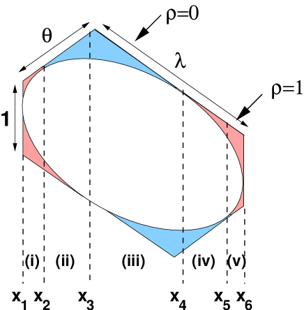
The general picture is summarized in Fig.6. The density $\rho$ varies only within the ellipse inscribed inside the hexagon. The points where the ellipse touching the boundary of the hexagon have $x$-coordinates $x_{1}=0$ and $x_{6}=\lambda+\theta$ (vertical tangents), $x_{2}={\theta\over 1+\lambda}$, $x_{3}={\lambda\over 1+\theta}$, $x_{4}={\theta(1+\lambda+\theta)\over 1+\theta}$, and $x_{5}={\lambda(1+\lambda+\theta)\over 1+\lambda}$, with $x_{1}\leq x_{2}\leq x_{3}\leq x_{4}\leq x_{5}\leq x_{6}$. They correspond, respectively, to $b=a$, $b=1+x$, $a=0$, $b=1+\theta$, and $a=x-\lambda$.

The limit density is constant outside of the ellipse Fig.6 and is given by:

(i) $x\in[x_{1},x_{2}]$: top and bottom $\rho=1$

(ii) $x\in[x_{2},x_{3}]$: top $\rho=0$, bottom $\rho=1$

(iii) $x\in[x_{3},x_{4}]$: top and bottom $\rho=0$

(iv) $x\in[x_{4},x_{5}]$: top $\rho=1$, bottom $\rho=0$

(v) $x\in[x_{5},x_{6}]$: top and bottom $\rho=1$.

The explicit expressions for $\rho$ inside $[a,b]$ are given by eq.(3.4) in the cases (i) and (v), eq.(3.5) in the case (ii), eq.(3.3) in the case (iii), and eq.(3.6) in the case (iv).

4. Comparison with the general results of Kenyon-Okounkov-Sheffield

4.1. Equations for the slope

4.1.1.

Limit shapes for rhombi tilings and more generally for dimer models on bipartite graphs are known to be solutions to certain variational problem [1][5]. They minimize the rate functional which is determined by the free energy of the system on a torus.

Assume we have a polygonal region with sides $s_{1},\dots,s_{3d}$ of lengths $N_{1},\dots,N_{3d}$ parallel to the axes of the triangular lattice, such that three possible axes of the lattice alternate in the sequence $s_{i}$. Consider random tilings of such region with the probability $\propto q^{vol(h)}$ where $h$ is the height function corresponding to the tiling. When $q\to 1$ such that $q^{-\epsilon c}$ and $\epsilon N_{i}$ are kept finite random tilings develop the limit shape at the macroscopical scale [4]. Moreover in this case the limit shape is described by an algebraic curve which can be explicitly constructed from the geometric data of the region.

Recall that rhombus tilings of a simply connected domain are in a bijection with the height functions (certain discrete surfaces in 3D over this domain). When the domain is not simply connected the height function does not exist but what would be its gradient still makes sense. It is called the slope of the tiling. The slope describes the local proportions of tiles of types $a,b,c$ as follows. Consider the tiling of a toroidal domain of fixed size, let $N_{a},N_{b},N_{c}$ be the numbers of tiles used in the tiling with $N=N_{a}+N_{b}+N_{c}$, then the slope is defined as $(s,t)=\nabla h=(h_{x},h_{y})=(N_{a}/N,N_{b}/N)$ (here, $x,y$ refer to coordinates in a basis $(u,v)$, with $u^{2}=v^{2}=1$ and $u.v=-1$).

4.1.2.

As explained in [5][4] there are two natural complex functions on the domain in question, $z$ and $w$ parameterizing the height function:

(4.1) $$\nabla h={1\over\pi}\left({\rm Arg}(-w),{\rm Arg}(-{1\over z})\right)$$

In the limit when $q\to 1$ and the regions increase at the consistent rate (see above), these variables satisfy the system of equations:

$$P(z,w) = 0$$

$${\rm Re}(z_{x}/z+w_{y}/w) = c$$

for some constant $c$. In addition $z$ and $w$ should satisfy the boundary conditions determined by the geometry of the region and restrictions on tilings.

The function $P(z,w)$ is polynomial for periodically weighted lattices. It is the determinant of the Kasteleyn matrix with quasiperiodic boundary conditions which is the partition function of the dimer model on the(toroidal) fundamental domain of its weights.

In our case

$$P(z,w)=1+z+w.$$

Solving the system for $z$ and $w$ by complex characteristics we change it to the system of equations

(4.2) $$P(z,w) = 0$$

(4.3) $$Q(e^{-cx}z,e^{-cy}w) = 0$$

The function $Q$ is an analytic function, which depends on the boundary of the region.

When the region is polygonal, the function $Q$ is polynomial. It can be computed according to the description of [4] (Section 3.3.3).

One of the remarkable phenomena we observe in tilings of large domains is the existence of the frozen regions near the boundary. In these regions the height function is linear. In the case of rhombus tilings of a hexagon, the curve separating the frozen part and the disordered phase (where the height function varies smoothly) is an ellipse [2], and it was called the arctic circle. In [4] such curves are called clout curves. One of the important corollaries is that for polygonal regions such curves are real algebraic in $e^{cx},e^{cy}$. It is also important that they form a family of curves as one varies $c$.

When $c\to 0$, the second equation in (4.2) becomes $Q(z,xz+yw)=0$.

The arctic circle (the boundary of the limit shape) in the case of polygonal region is an algebraic curve intersecting each linear piece of the boundary once where it is tangent to the boundary. It may develop cusps. It may also be disconnected, i.e. it may have ”islands” and bubbles” (in the terminology of [4]), see Fig. 5, fig. 17 from [4].

4.2. Case of the cut hexagon

As explained before, the limiting density of exit points of LGV paths on a large cut hexagon $k\times n\times n$ with $n/k=\lambda$ fixed, $k\to\infty$ is identical to that of passing points of LGV paths through the main diagonal (which is where we make the cut). These paths describe the rhombus tilings of the hexagon which is obtained from the cut hexagon by gluing to the reflection w.r.t. the cut. In the language of [4], this density is the density of tilted rhombi and is determined by the limit shape of rhombus tilings of the complete hexagon.

For the unweighted tilings by rhombi we have $P(z,w)=1+z+w$. The polynomial $Q$ for such tiling of the hexagon has degree $2$ ( half of the number of sites of the region) and reads:

$$Q(z,xz+yw)=\lambda^{2}(z+z^{2})-(xz+yw)^{2}-(1+\lambda)(xz+yw)$$

The equations (4.2) for $c=0$ become quadratic equation for $z$:

$$(\lambda^{2}-(x-y)^{2})z^{2}+(\lambda^{2}-(1+\lambda-2y)(x-y))z+y(1+\lambda-y)=0$$

The arctic circle is the curve in $(x,y)$ on which the discriminant of this equation vanishes:

$$0 = (\lambda^{2}-(1+\lambda-2y)(x-y))^{2}-4y(1+\lambda-y)(\lambda^{2}-(x-y)^{2})$$

$$= (1+2\lambda)(x-y)^{2}+\lambda^{2}(x+y-\lambda-1)^{2}-\lambda^{2}(1+2\lambda)$$

It is tangent to the six edges of the hexagon, namely $y=0,y=\lambda+1$, $x=0,x=\lambda+1$, and $y=x\pm\lambda$. This curve intersects the reflection axis $y=x$ (the cut) at points $x={\lambda+1\over 2}\pm{\sqrt{1+2\lambda}\over 2}$ which coincide with the ends of the support of $\rho$ .

The passing points of the LGV paths along the cut correspond to tiles of type $a$ or $b$. The local density of such tiles is therefore $(N_{a}+N_{b})/N=h_{x}+h_{y}$. Hence the density (3.3) should be compared to the “vertical” slope $h_{x}+h_{y}$ in our solution.

Solving for $z$ at $y=x$, we find that $\lambda^{2}(z+{1\over 2})^{2}=(x-{1+\lambda\over 2})^{2}-{1+2\lambda\over 4}$, so that:

$$z = {1\over 2}\left(-1\pm\sqrt{(x-a)(x-b)\over ab}\right)$$

$$w = {1\over 2}\left(-1\mp\sqrt{(x-a)(x-b)\over ab}\right)$$

and finally we get

$$h_{x}=h_{y}={1\over\pi}{\rm Arctan}\,\sqrt{(b-x)(x-a)\over ab}$$

and therefore $\rho(x)=h_{x}+h_{y}$ as expected.

4.3. Case of the full hexagon

Here we will compare the results of previous sections with the computation of the limit shape based on the equation (4.2).

In the case of the full hexagon with edges $1,\lambda,\theta$ the equations (4.2) becomes

$$0 = 1+z+w$$

$$0 = \lambda\theta(z+z^{2})-(xz+yw)^{2}-(\lambda-\theta)z(xz+yw)-(1+\lambda)(xz+yw)$$

The arctic curve appear as the condition that the discriminant of this equation vanishes. It is the ellipse:

(4.4) $${\Big{(}(1+\lambda)x+(1+\theta)y-(1+\lambda)(1+\theta)\Big{)}^{2}\over 1+\lambda+\theta}+{\Big{(}(1+\lambda)x-(1+\theta)y\Big{)}^{2}\over\lambda\theta}=(1+\lambda)(1+\theta)$$

tangent to respectively $x=0$, $x=\theta$, $y=0$, $y=\lambda$, $y=x+\lambda$ and $y=x-\theta$.

To get the density of LGV points, let us solve for $z$ on some arbitrary vertical line $y=x+t$. It is easy to see that the line crosses the arctic curve at the points

$$x_{\pm}=\left({\sqrt{\lambda(t+\theta)}\mp\sqrt{\theta(\lambda-t)(1+\lambda+\theta)}\over\lambda+\theta}\right)^{2}$$

These are identified with the ends of the support of $\rho$ given in eq.(3.2), namely $x_{-}=a$ and $x_{+}=b$, upon the substitution $x=\lambda-t$. The solution for $z$ reads:

$$z=-{1\over 2(t+\theta)(\lambda-t)}\left(t+(\lambda-t-x)(t+\theta)+(\lambda-t)(t+x)\pm(\lambda+\theta)\sqrt{(x-a)(x-b)}\right)$$

and we finally get

$$h_{x} = {1\over\pi}{\rm Arctan}\,{(\lambda+\theta)\sqrt{(b-x)(x-a)}\over(\lambda-t-x)(t+\theta)+t+(\lambda-t)(t+x)}$$

$$h_{y} = {1\over\pi}{\rm Arctan}\,{(\lambda+\theta)\sqrt{(b-x)(x-a)}\over(\lambda-t+x)(t+\theta)-t-(\lambda-t)(t+x)}$$

Using the addition formula for Arctan, we finally get

(4.5) $$h_{x}+h_{y}={1\over\pi}{\rm Arctan}\,{(\lambda+\theta)\sqrt{(b-x)(x-a)}\over\lambda\theta-t(1+\theta)+2x(x+t-1-{\lambda+\theta\over 2})}$$

To compare this with the results on the LGV point densities, let us assume for definiteness that we have $x_{3}<x<x_{4}$ (case (iii)), namely ${\lambda\over 1+\theta}-\theta<t<{\lambda\theta\over 1+\theta}$. Using eqs. (3.2) and (3.9) and the restriction on $t$, we find that

$$\sqrt{1+\theta-a\over 1+\theta-b} = {\sqrt{\theta(\theta+t)(1+\lambda+\theta)}+\sqrt{\lambda(\lambda-t)}\over\sqrt{\theta(\theta+t)(1+\lambda+\theta)}-\sqrt{\lambda(\lambda-t)}}$$

$$\sqrt{a\over b} = {\sqrt{\theta(\lambda-t)(1+\lambda+\theta)}-\sqrt{\lambda(\theta+t)}\over\sqrt{\theta(\lambda-t)(1+\lambda+\theta)}+\sqrt{\theta(\theta+t)}}$$

$$\sqrt{1+x-a\over 1+x-b} = {\sqrt{\lambda(\lambda-t)(1+\lambda+\theta)}+\sqrt{\theta(\theta+t)}\over\sqrt{\lambda(\lambda-t)(1+\lambda+\theta)}-\sqrt{\theta(\theta+t)}}$$

$$\sqrt{\lambda-x+a\over\lambda-x+b} = {\sqrt{\lambda(\theta+t)(1+\lambda+\theta)}-\sqrt{\theta(\lambda-t)}\over\sqrt{\lambda(\theta+t)(1+\lambda+\theta)}+\sqrt{\theta(\lambda-t)}}$$

We use the subtraction/addition formulae for Arctan to get:

$${\rm Arctan}\,\sqrt{b-z\over z-a}\sqrt{1+x-a\over 1+x-b}-{\rm Arctan}\,\sqrt{b-z\over z-a}\sqrt{a\over b}={\rm Arctan}\,{\sqrt{(b-z)(z-a)}(\lambda+\theta)\over\theta\lambda-t(1+\theta)+z(\lambda-\theta)}$$

$${\rm Arctan}\,\sqrt{b-z\over z-a}\sqrt{1+\theta-a\over 1+\theta-b}-{\rm Arctan}\,\sqrt{b-z\over z-a}\sqrt{\lambda-x+a\over\lambda-x+b}={\rm Arctan}\,{\sqrt{(b-z)(z-a)}(\lambda+\theta)\over\theta\lambda+t(1+\theta)-z(\lambda-\theta)}$$

and finally

$$\rho(z) = {1\over\pi}\left({\rm Arctan}\,{\sqrt{(b-z)(z-a)}(\lambda+\theta)\over\theta\lambda-t(1+\theta)+z(\lambda-\theta)}+{\rm Arctan}\,{\sqrt{(b-z)(z-a)}(\lambda+\theta)\over\theta\lambda+t(1+\theta)-z(\lambda-\theta)}\right)$$

$$= {1\over\pi}{\rm Arctan}\,{\sqrt{(b-z)(z-a)}(\lambda+\theta)\over\theta\lambda-t(1+\theta)+2z(z+t-1-{\lambda+\theta\over 2})}$$

in agreement with (4.5).

The other cases follow analogously.

5. Symmetries

Figure 7. A cut hexagon with zig-zag fixed boundary.

5.1. Case of a cut hexagon with a fixed zig-zag boundary

5.1.1.

The “half” cut hexagon (see Fig.7), of the size $k\times 2n\times 2n+k$ is another case when the total number of lattice path configurations nicely factorizes. In this case the lattice paths start at each point of the left boundary and ends on the right boundary. The low boundary is a horizontal zig-zag line.

The LGV formula expresses the total number of configurations of such non-intersecting paths, which start at $(0,2i-2)$, $i=1,2,...,k$, and end at $(2n,2m_{j}-2)$, $j=1,2,...,k$, $1\leq m_{j}\leq k+n$ as the determinant: det${}_{1\leq i,j\leq k}(p_{i,m_{j}}^{(n)})$. Here $p_{i,m}^{(n)}$ is the numbers of paths from $(0,2i-2)$ to $(2n,2m-2)$. By the standard reflection principle, this number $p_{i,m}^{(n)}$ is exactly the number of unrestricted paths from $(0,2i-2)$ to $(2n,2m-2)$ minus the number of of unrestricted paths from $(0,-2i)$ to $(2n,2m-2)$:

$$p_{i,m}^{(n)}={2n\choose n+m-i}-{2n\choose n+m+i-1}$$

Finally we have the factorization formula

(5.1) $$\tilde{Z}_{k,n}(\{{\mathbf{m}}\})=\det_{1\leq i,j\leq k}(p_{i,m_{j}}^{(n)})=\prod_{i=1}^{k}{(2n+2i-2)!\over(n+m_{i}+k-1)!(n-m_{i}+k)!}\\ \,\prod_{1\leq i<j\leq k}(m_{j}-m_{i})\,\prod_{1\leq i\leq j\leq k}(m_{i}+m_{j}-1)$$

Let us now compute the asymptotic of this number, when $k\to\infty$, and say $n/k={\alpha}$ fixed, while $\mu_{i}=m_{i}/k$ converges to a continuous function on $[0,1]$, or equivalently gets distributed on $[0,\alpha+1]$ with the limit density $\rho(\mu)$.

We have

(5.2) $$-{1\over k}{\rm Log}(\tilde{Z}_{k,n}(\{{\mathbf{m}}\}))=C+{1\over k}\sum_{i=1}^{k}(({\alpha}+1+\mu_{i})\,{\rm Log}({\alpha}+1+\mu_{i})+\\ ({\alpha}+1-\mu_{i})\,{\rm Log}({\alpha}+1-\mu_{i}))-{1\over k^{2}}\sum_{i<j}{\rm Log}|\mu_{j}^{2}-\mu_{i}^{2}|$$

for some constant $C$ depending only on ${\alpha}$. As $k\to\infty$ this gives the action (the rate functional)

(5.3) $$S[\rho]=C+\int_{0}^{\alpha+1}(({\alpha}+1+\mu)\,{\rm Log}({\alpha}+1+\mu)+({\alpha}+1-\mu)\,{\rm Log}({\alpha}+1-\mu))\rho(\mu)d\mu-\\ \int_{0}^{\alpha+1}\int_{0}^{\alpha+1}{\rm Log}|\mu^{2}-\nu^{2}|\rho(\mu)\rho(\nu)d\mu d\nu$$

Fixed points of this functional are solutions to the integral equation

$${\rm Log}\,{{\alpha}+1+\mu\over{\alpha}+1-\mu}=\mathchoice{{\vbox{\hbox{$\textstyle-$}}\kern-4.86108pt}}{{\vbox{\hbox{$\scriptstyle-$}}\kern-3.25pt}}{{\vbox{\hbox{$\scriptscriptstyle-$}}\kern-2.29166pt}}{{\vbox{\hbox{$\scriptscriptstyle-$}}\kern-1.875pt}}\!\int_{0}^{\alpha+1}\left({1\over\mu-u}+{1\over\mu+u}\right)\sigma(u)du$$

subject to the constraint $\int_{0}\sigma(u)du=1$. As before assume the density is zero for $z\in[a,\alpha+1]$. It is convenient to extent the problem to the symmetric interval $[-a,a]$ assuming that $\sigma(z)$ is extended as a symmetric function $\sigma(z)=\sigma(-z)$. The integral equation becomes

$${\rm Log}\,{{\alpha}+1+\mu\over{\alpha}+1-\mu}=\mathchoice{{\vbox{\hbox{$\textstyle-$}}\kern-4.86108pt}}{{\vbox{\hbox{$\scriptstyle-$}}\kern-3.25pt}}{{\vbox{\hbox{$\scriptscriptstyle-$}}\kern-2.29166pt}}{{\vbox{\hbox{$\scriptscriptstyle-$}}\kern-1.875pt}}\!\int_{-a}^{a}{1\over\mu-u}\sigma(u)du$$

with the constraint $\int_{-a}^{a}\sigma(u)du=2$.

Similarly to previous sections it is easy to obtain an explicit formula for the resolvent $G(z)=\int_{-a}^{a}{1\over\mu-u}\sigma(u)du$:

$$G(z)={1\over\pi}\sqrt{z^{2}-a^{2}}\int_{a}^{a}{1\over\sqrt{u^{2}-a^{2}}}{\rm Log}\,{{\alpha}+1+u\over{\alpha}+1-u}{du\over z-u}$$

The constraint on the density is equivalent to the condition $G(z)={2\over z}+O({1\over z^{2})}$ as $z\to\infty$. Solving this, we arrive to $a=\alpha+1-{\sqrt{3+4\alpha}\over 2}$. Combining this with the explicit evaluation of the integral for $G(z)$ we obtain the limit density:

(5.4) $$\sigma(z)={2\over\pi}\,{\rm Arctan}\,{\sqrt{3+4{\alpha}-4z^{2}}\over 1+2{\alpha}}$$

for $z\in[0,\sqrt{{3\over 4}+{\alpha}}]$ and $\sigma(z)=0$ for $z>\sqrt{{3\over 4}+{\alpha}}$.

5.1.2.

We could have found this result a priori, by recognizing that the half-cut hexagon from the previous section is the fundamental domain for the obvious reflection symmetry of the cut hexagon from the first section.

Because the limit density is the unique minimizer of the rate functional, it is invariant with respect to this reflection. In terms of the limit density or the cut hexagon from section 1 this is the symmetry $\rho(z)=\rho(\lambda+1-z)$.

Taking into account the change of variables from Fig. 1 to Fig. 7 we can see that indeed

$$\rho(z+\alpha+1)=\sigma(z)$$

where $\lambda+1=2(\alpha+1)$, $\rho(t)$ is given by (1.15) and $\sigma(z)$ is by (5.4).

5.2. The reflection principle for limit densities

5.2.1.

The reflection principle which was illustrated above can be used to compute the limit density for a random tiling along the free boundary in a more general setting. In particular, it can be used to compute such density from the limit shape on doubled domain with fixed boundary.

Assume that the free boundary of a domain $\mathcal{D}$ is a collection of segments on a line and let ${\mathcal{D}}^{r}$ be the reflection with respect to this line. The doubled domain ${\mathcal{D}}\cup{\mathcal{D}}^{r}$ is closed with feasible (in a sense of [4]) boundary. It is invariant with respect to the reflection ${\mathcal{D}}\to{\mathcal{D}}^{r}$. If we extend the definition of weights of tiling to ${\mathcal{D}}^{r}$ such that the weights will also be invariant with respect to this reflection, the resulting limit shape density will also be invariant. It is also clear that in this case the limit shape density for tilings of the domain ${\mathcal{D}}\cup{\mathcal{D}}^{r}$ at the symmetry axis is the same as the the limit density for the tilings of ${\mathcal{D}}$ with the free boundary condition along this axis. Thus, the problem of computing the density of tiles at the free boundary reduces to the computation of the limit shape for a symmetric domain with fixed boundary along the symmetry axis.

As an example we can compare the limit density at the diagonal of the symmetric hexagon with $\lambda=\theta$ with the density at the free boundary of the cut hexagon with the same value of $\lambda$. The symmetry axis of the hexagon correspond $x=\lambda$ in the computation of the density along slices of the hexagon. The density along this line is given by eq.(3.3) with $x=\theta=\lambda$, and with $a$ and $b$ given by eq.(3.2). These expressions for the hexagon case are identical to formulae (1.13)(1.15)for the density of endpoints of lattice paths along the free boundary for the half-hexagon of the same shape.

Figure 8. The regular hexagon is decomposed into six triangles (a). The two inner boundaries are both parts of lines that divide the hexagon in two (dashed lines), each corresponding to cuts along lattice paths made of the two indicated tiles, for which the density along the cut is known. In (b) we interpret the tiling of the triangle in terms of lattice paths starting at the fixed edge and ending on the two free inner boundaries, along the third type of edge, not used for the paths in (a). In (c), the same tiling is now interpreted differently in terms of paths that start on the lower free boundary via tiles of the third type, and end on the top one with the two first type of tiles.

5.2.2.

Now let us discuss limit shapes corresponding to lattice paths in the cut hexagon with forbidden intervals along the cut.

Lattice paths and equivalent to tilings by rhombi which is also equivalent to monotonic piles of unit cubes in the corner of a “3D-room”. This is simply another way to phrase that rhombus tiling configurations are equivalent to the corresponding height functions.

Figure 9. The 3D realization of forbidden (a) and fully packed (b) boundaries. Both are obtained by removing from the large parallelepiped (the room, in dashed lines) two smaller ones touching opposite corners of the room. In the case (a), they share a plane domain (a square in the case of regular objects), while in case (b) they intersect along a segment. The diagonal of the square and the segment, in projection, correspond to respectively the forbidden interval and the fully packed one. We have also represented the expected limit shapes for the associated rhombus tilings.

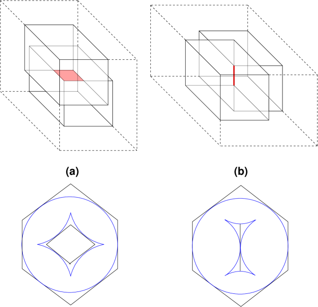
The case of the cut hexagon with one forbidden interval corresponds to pile of cubes in a rectangular room with two parallelepipeds removed from it (see Fig.9 (a)). One is removed from the upper closest corner, one is removed from the lower corner of the other side. They should have the complementary heights (their sum is equal to the height of the room) and they projections on the $(x,y)$ plane should intersect. If this configuration is symmetric with respect to the reflection $(x,y)\to(y,x)$, the lattice paths corresponding to such a pile of cubes will have the forbidden interval along the diagonal of the square which is the intersection of the lower side of the upper parallelepiped and the upper side of the lower parallelepiped. If we cut this rectangular room along the diagonal, the corresponding lattice paths will be exactly lattice paths in the cut hexagon with a forbidden interval along the cut.

In this case the density of the LGV paths along the cut is determined by the limit slope of the corresponding tilings, or equivalently by the limit height of corresponding piles of cubes. The boundary of the limit shape in this case is disconnected. In terminology [4] this limit shape is the result of the degeneration of the island with the hexagon inside and six cusps. The degeneration “flattens” the hexagon to a rhombus with horizontal main diagonal (two vertical sides shrink to points). As a result six cusps around the hexagonal island degenerate into four cusps around the rhombus.

A similar interpretation holds for the density of end points of lattice paths with fully packed interval along the free boundary of the cut hexagon. In this case piles of cubes also should be in the a 3D rectangular room with two parallelepipeds removed from it (see Fig.9 (b)). As in the case of forbidden intervals, one of them is removed from the upper closest corner, one is removed from the lower corner of the other side. The difference is that their projections on the $(x,y)$ plane should be complementary (they should intersect over exactly one point). The sum of heights should be greater then the height of the room. In this case parallelepipeds intersect over a vertical segment. When such a configuration is symmetric with respect to the reflection $(x,y)\to(y,x)$, the piles of cubes in such room with removed parallelepipeds are equivalent to the lattice paths on the left side continuing to the lattice paths on the right side with the fully packed interval at the diagonal cut (the interval where two parallelepipeds intersect).

In this case the limit shape will be discontinuous. In the terminology of [4] this case is also a degeneration of an island but the hexagon now becomes ”squashed” sidewise such that it degenerates to a vertical segment (tilted sides degenerate to points). In this case six cusps also degenerate to four cusps.

5.2.3.

This symmetry principle extends to situations with other symmetries. Consider for instance a regular hexagon (corresponding to $\lambda=\theta=1$ in the previous section). Then the domain is invariant under rotations by $2\pi/3$, and reflections w.r.t. axes joining opposite vertices. Let us cut the hexagon into six triangles according to these symmetries, and focus on one of them (see Fig.8 (a)).

The counter clock-wise rotation by $2\pi/3$ brings a tiling to a tiling. It maps the square looking tiles from the upper side of the triangle from Fig. 8(c) to the tiles along the lower side of the triangle from Fig. 8(b) where lattice paths end.

Because the hexagon is invariant with respect to rotations, because the action function (the entropy, or the rate function) is invariant with respect to such rotations, and because it has unique minimizer the limit hight function is also invariant with respect to such rotations, if one takes into account that the rotations also rotate tiles.

In particular , if $\sigma(z)$ is the density of lattice paths along the lower boundary of the triangle from Fig. 8(c) and $\rho(z)$ is the density of paths along the upper boundary of the same triangle, we have $\rho(z)=1-\sigma(z)$. Here $z$ is the distance from the right lower corner.

The density $\rho(z)$ we computed earlier in eq. (1.15) for all values of $\lambda$. For $\lambda=1$ we have:

(5.5) $$\rho(z)=\left\{\begin{matrix}0&z\in[0,1-\frac{\sqrt{3}}{2}]\\ {2\over\pi}\,{\rm Arctan}\,\sqrt{3-4(z-1)^{2}}&z\in[1-\frac{\sqrt{3}}{2},1]\end{matrix}\right.$$

Here $z$ is the coordinate along the upper side of the triangle with $z=0$ being the upper corner and $z=1$ being the lower right corner.

For the density $\sigma(z)$ we obtain

(5.6) $$\sigma(z)=\left\{\begin{matrix}1&z\in[0,1-\frac{\sqrt{3}}{2}]\\ {2\over\pi}\,{\rm Arctan}\,\sqrt{1\over\sqrt{3-4(z-1)^{2}}}&z\in[1-\frac{\sqrt{3}}{2},1]\end{matrix}\right.$$

More generally, from the results for lattice paths in a hexagon, we obtain the density of the lattice paths in the triangle from Fig. 8(c). Let $L_{x}$ be the line parallel to the upper side of the triangle which is at the distance $x$ from the left lower corner. In the formulae below we use the coordinate $z$ which is $0$ at the left side of the triangle and changes from $0$ to $x$ along $L_{x}$ as we move downward. Let $\rho(z,x)$ be the density of paths crossing $L_{x}$, $0\leq z\leq x$.

For $0\leq x\leq 1-\frac{\sqrt{3}}{2}$ we have $\rho(z,x)=1$ for all $0\leq z\leq x$.

For $1-\frac{\sqrt{3}}{2}\leq x\leq\frac{1}{2}$ and $z\in[0,a]$ we have $\rho(z,x)=1$ and

(5.7) $$\rho(z,x) = 1+{1\over\pi}\left({\rm Arctan}\,\sqrt{b-z\over z-a}\sqrt{1+\theta-a\over 1+\theta-b}-{\rm Arctan}\,\sqrt{b-z\over z-a}\sqrt{1+x-a\over 1+x-b}\right.$$

$$\qquad\qquad\left.+{\rm Arctan}\,\sqrt{b-z\over z-a}\sqrt{a\over b}-{\rm Arctan}\,\sqrt{b-z\over z-a}\sqrt{\lambda-x+a\over\lambda-x+b}\right)$$

when $z\in[a,x]$. Here $a=\frac{1+x}{2}-\frac{1}{2}\sqrt{(2-x)3x}$ and $b=\frac{1+x}{2}+\frac{1}{2}\sqrt{(2-x)3x}$.

For $\frac{1}{2}\leq x\leq 1$, we have $\rho(z,x)=0$ when $0\leq z\leq a$ and

(5.8) $$\rho(z,x) = {1\over\pi}\left({\rm Arctan}\,\sqrt{b-z\over z-a}\sqrt{1+\theta-a\over 1+\theta-b}+{\rm Arctan}\,\sqrt{b-z\over z-a}\sqrt{1+x-a\over 1+x-b}\right.$$

$$\qquad\qquad\left.-{\rm Arctan}\,\sqrt{b-z\over z-a}\sqrt{a\over b}-{\rm Arctan}\,\sqrt{b-z\over z-a}\sqrt{\lambda-x+a\over\lambda-x+b}\right)$$

These formulae compare with eq. (5.5) as $\rho(z)=\rho(z,1)$.

5.2.4. Limit shape of TSSCPP

Figure 10. TSSCPP are the rhombus tilings of a half-equilateral triangle, with fixed boundary along the half-edge and the zig-zag median, and free boundary along the remaining edge. We have indicated with dots the starting and ending points of the non-intersecting paths with a floor, in bijection with the tilings. The exit tiles are those marked by dots along the free boundary. We expect the zig-zag line to become the reflection symmetry axis of the full equilateral triangle in the continuum.

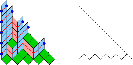
The Totally Symmetric Self-Complementary Plane Partitions (TSSCPP) are in bijection with the tilings of a half equilateral triangle of edge size $2n$, with fixed straight boundary along one edge, fized zig-zag boundary along the median perpendicular to that edge, and free boundary along the remaining edge (see Fig.10).

The region in this problem can be naturally identified with the fundamental domain of the full, fully symmetric hexagon. It is natural to choose it as the triangle with $0\leq x\leq 1$ and $x\leq z\leq\frac{1+x}{2}$. Under this identification the zig-gag line becomes the line $z=x$. As $n\to\infty$ it becomes the symmetry axis of the limit shape of the height function for the equilateral hexagon.

Using the same symmetry arguments as above we can compute the limit density of paths crossing the vertical line $L_{x}$ which is at the distance $x$ from the left side of the triangle. Denote this density by $\sigma(z,x)$.

When $0\leq x\leq 1-\frac{\sqrt{3}}{2}$ we have $\sigma(z,x)=1$ for $0\leq z\leq a$ and $\sigma(z,x)$ is given by eq. (5.7) for $a\leq z\leq\frac{1+x}{2}$.

When $1-\frac{\sqrt{3}}{2}\leq x\leq 1/2$ the density is given by eq. (5.7) for all $x\leq z\leq\frac{1+x}{2}$. It is given by eq. (5.7) for all $x\leq z\leq\frac{1+x}{2}$ when $1/2\leq x\leq 1$.

These expressions agree with the function eq. (5.6): $\sigma(x,x)=\sigma(x)$.

5.3. Some other examples

Figure 11. Various applications of the symmetry principle, to a hexagon with two free boundaries.

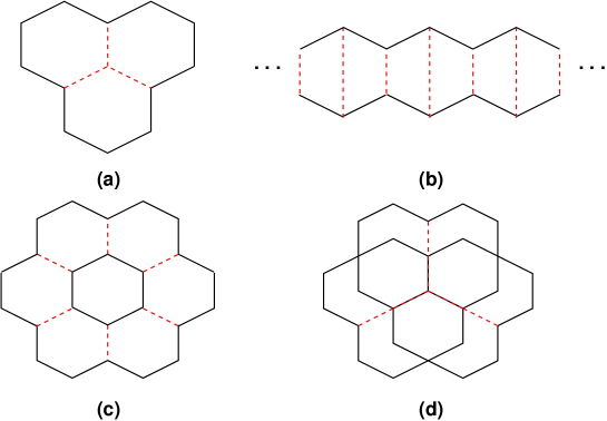
Another example of the application of the symmetry principle is the computation of the limit shape for the equilateral hexagonal region with free boundary condition on two adjacent sides. In this case one should glue three such hexagons into the region shown on Fig.11(a). The limit shape for this region can be found using the methods of [4].

The cut hexagon with both sides having free boundary conditions on tilings correspond to a random tiling of the infinite region obtained by gluing infinitely many hexagons along vertical boundaries Fig.11(b). This case also describes the hexagon where two opposite sides have the free boundary.

For more complicated examples of regions with free boundaries the corresponding region with fixed boundary may not be simply connected (see Fig.11(c)), nor planar (see Fig.11(d)).

References

• [1] H. Cohn, R. Kenyon, and J. Propp, A variational principle for domino tilings, J. Amer. Math. Soc. 14 (2001) 297–346, arXiv:math/0008220 [math.CO].
• [2] H. Cohn, M. Larsen, and J. Propp, The shape of a typical boxed plane partition, New York J. Math. 4 (1998) 137–165, arXiv:math/9801060 [math.CO].
• [3] I. M. Gessel and X. Viennot, Binomial determinants, paths and hook formulae, Adv. Math. 58 (1985) 300–321.
• [4] R. Kenyon and A. Okounkov, Limit shapes and the complex Burgers equation, Acta Math. 199 (2007), no. 2, 263–302, arXiv:math-ph/0507007.
• [5] R. Kenyon, A. Okounkov, and S. Sheffield, Dimers and amoebae, Ann. of Math. (2) 163 (2006), no. 3, 1019–1056, arXiv:math-ph/0311005.
• [6] B. Nienhuis, H. Hilhorst, and H.W.J. Blöte, Triangular SOS models and cubic-crystal shapes, J. Phys. A 17 (1984), no. 18, 3559–3581.
• [7] G. Andrews, Plane Partitions V: the TSSCPP conjecture, J. Combin. Theory Ser. A 66 (1994) 28–39.