Accretion Rates of Planetesimals by Protoplanets Embedded in Nebular Gas

Abstract

When protoplanets growing by accretion of planetesimals have atmospheres, small planetesimals approaching the protoplanets lose their energy by gas drag from the atmospheres, which leads them to be captured within the Hill sphere of the protoplanets. As a result, growth rates of the protoplanets are enhanced. In order to study the effect of an atmosphere on planetary growth rates, we performed numerical integration of orbits of planetesimals for a wide range of orbital elements and obtained the effective accretion rates of planetesimals onto planets that have atmospheres. Numerical results are obtained as a function of planetesimals’ eccentricity, inclination, planet’s radius, and non-dimensional gas-drag parameters which can be expressed by several physical quantities such as the radius of planetesimals and the mass of the protoplanet. Assuming that the radial distribution of the gas density near the surface can be approximated by a power-law, we performed analytic calculation for the loss of planetesimals’ kinetic energy due to gas drag, and confirmed agreement with numerical results. We confirmed that the above approximation of the power-law density distribution is reasonable for accretion rate of protoplanets with one to ten Earth-masses, unless the size of planetesimals is too small. We also calculated the accretion rates of planetesimals averaged over a Rayleigh distribution of eccentricities and inclinations, and derived a semi-analytical formula of accretion rates, which reproduces the numerical results very well. Using the obtained expression of the accretion rate, we examined the growth of protoplanets in nebular gas. We found that the effect of atmospheric gas drag can enhance the growth rate significantly, depending on the size of planetesimals.

Keywords: planetary formation; planetesimals; origin, solar system

1 Introduction

Planets are thought to be formed in circum-stellar gas disks by accumulating a large number of planetesimals. When a protoplanet reaches about the Moon mass, it starts to attract surrounding gas of the disk by its gravity, which would lead to the formation of a thick atmosphere, if the growth of the protoplanet proceeds in the nebular gas. Thus, in the process of planetesimal accretion onto planets, interactions between planetesimals and atmospheres should be considered. Interactions between planetary atmospheres and planetesimals have been studied mainly in the context of giant planet formation. Podolak et al. (1988) studied the interaction of planetesimals with atmospheres in order to examine the ablation and dissolution of incoming planetesimals due to gas drag by calculating trajectories and mass-loss rates of the planetesimals. Pollack et al. (1996) and Hubickyj et al. (2005) followed the method of Podolak et al. (1988) to calculate energy and mass deposition on the atmosphere when planetesimals are passing through it as a part of their formation model of giant planets. Also, in relation to the origin of natural satellites, the interaction between primordial atmospheres and incoming objects was considered, in order to study the possibility of capture of satellites by the gas drag, as well as the orbital evolution of captured satellites (Pollack et al., 1979; Ćuk and Burns, 2004).

Interactions between planetesimals and atmospheres also affect the growth rate of protoplanets. In protoplanetary disks, solid protoplanets form first, and then solid protoplanets with a sufficiently large mass (about $\gtrsim$ 10 Earth masses) acquire a large amount of gas to become gas-giant protoplanets (Mizuno, 1980; Bodenheimer and Pollack, 1986; Pollack et al., 1996; Ikoma et al., 2000; Hubickyj et al., 2005). This scenario is widely accepted, but the growth timescale of solid planets predicted by results of theoretical studies of planetary accretion (e.g., Tanaka and Ida, 1999; Kokubo and Ida, 2000) are too long in two senses. First, the predicted growth timescale is longer than the typical timescale of inward migration of protoplanets predicted by current theories including linear analyses (e.g., Ward, 1986, 1997; Korycansky and Pollack, 1993; Tanaka et al., 2002) and numerical simulations (e.g., D’Angelo et al., 2002; Masset et al., 2006), which results in the loss of forming planets into the central star before the completion of their growth. Second, planets cannot reach a critical mass that is necessary for the onset of runaway gas accretion before dissipation of disk gas, which means that gas giant planets are difficult to be formed. Current theories predict that solid planets grow in proto-planetary disks via runaway growth phase (Wetherill and Stewart, 1989) followed by oligarchic growth phase (Kokubo and Ida, 1996), and in both phases, protoplanets grow mainly by capturing objects that are much smaller than the protoplanets. Thus, in order to estimate the growth timescale of solid planets, one has to investigate the stage where a large number of small objects are accreted by a small number of large objects.

Collision rates of small objects onto protoplanets have been studied in detail by numerical orbital integration and analytical calculations (Nishida, 1983; Wetherill and Cox, 1985; Ida and Nakazawa, 1989; Greenzweig and Lissauer, 1990, 1992; Dones and Tremaine, 1993). The early stage of planetary accretion is likely to have proceeded in the presence of the protoplanetary gas disk, but most of the previous studies did not consider the effect of atmosphere around protoplanets, which likely enhances effective accretion rates through gas drag. Kary et al. (1993) and Kary and Lissauer (1995) studied accretion rates when planetesimals are migrating radially inward by gas drag from the nebular gas, but they did not consider the effect of planets’ atmospheres.

Inaba and Ikoma (2003) first examined the effect of atmospheric gas drag on planetary accretion rates in detail. They showed that the presence of atmospheres around planets can enhance the accretion rate greatly depending on the size of objects that are passing through the atmospheres. The results were used in their simulation of planetary accretion in the Jovian region (Inaba et al., 2003). Chambers (2006a, b) also used the results of Inaba and Ikoma (2003) in his semi-analytic model of oligarchic growth of planets, and showed that the enhancement of the accretion rate can shorten the growth timescale so that gas giant planets can be formed before the dispersal of the gas disk, if incoming planetesimals are small ($\lesssim$ 100m). Although Inaba and Ikoma (2003) demonstrated the importance of the atmosphere for planetary accretion rates, most of their results were based on calculations neglecting the solar gravity, and three-body orbital integration was performed only in the case of initially circular orbits. In addition, they used a realistic model for the atmospheric structure rather than a simplified one, which makes the study of parameter-dependence or comparison with analytic calculations rather difficult.

In the present work, we obtain accretion rates of planetesimals onto protoplanets that have atmospheres, by using three-body orbital integration for a wide range of parameters. We use a simple power-law density distribution model for the atmosphere, which allows a systematic study of the accretion rate and its parameter-dependence. From the obtained accretion rates, we derive a semi-analytical expression of the accretion rates for planets with atmospheres and examine growth of protoplanets in the nebular gas. In §2, we first show the basic formulation and some analytic estimations which are the basis of our numerical simulation and analysis to obtain the accretion rates. In §3, we show the results of our numerical simulations to obtain the accretion rates, together with some demonstrative calculations, which are useful in understanding the basic behavior of planetesimals’ motion under the gas drag of planetary atmospheres. In §4, we derive a semi-analytic formula for accretion rates under the assumption of power-law density profile for atmospheres. In §5, we examine the validity of the power-law approximation for density profile of atmospheres. Using the obtained semi-analytic formula for accretion rates, we examine the growth of protoplanets with atmospheres in §6. Our conclusions and discussion are presented in §7.

2 Basic Formulation and Analytical Estimate

2.1 Basic equations

When the masses of planetesimals and the planet are much smaller than the solar mass and their orbital eccentricities and inclinations are sufficiently small, their motions in a rotating coordinate system can be described by linearized equations, called Hill’s equations. We use a coordinate system centered on the planet, where the $x$-axis points radially outwards, the $y$-axis points in the direction of the planet’s orbital motion, and the $z$-axis is normal to the $x$–$y$ plane. We scale the distance by the mutual Hill radius $r_{\rm H}\equiv ah$ with $h\equiv\{(M+m)/3M_{\ast}\}^{1/3}$ ($M$ and $m$ are the masses of the planet and a planetesimal, respectively; $a$ is the semi-major axis of the planet; and $M_{\ast}$ is the mass of the central star) and the time by $\Omega_{\rm K}^{-1}$ ($\Omega_{\rm K}$ is the planet’s orbital angular frequency). The non-dimensional equation for the relative motion between the planet and a planetesimal can then be written as

$$\frac{d\tilde{\mbox{\normalsize\boldmath$v$}}}{d\tilde{t}}=-\nabla\tilde{\Phi}-2\mbox{\normalsize\boldmath$e$}_{z}\times\tilde{\mbox{\normalsize\boldmath$v$}}+\tilde{\mbox{\normalsize\boldmath$a$}}_{\rm drag},$$ (1)

where $\tilde{\mbox{\normalsize\boldmath$v$}}$ is velocity, $\tilde{t}$ is time, and $\tilde{\Phi}$ is the Hill potential given by

$$\tilde{\Phi}=-\frac{3}{\tilde{r}}-\frac{3}{2}\tilde{x}^{2}+\frac{1}{2}\tilde{z}^{2}+\frac{9}{2},$$ (2)

where $\tilde{r}=\sqrt{\tilde{x}^{2}+\tilde{y}^{2}+\tilde{z}^{2}}$. Variables with tildes denote non-dimensional quantities. The acceleration due to gas drag $\tilde{\mbox{\normalsize\boldmath$a$}}_{\rm drag}$ is described by

$$\tilde{\mbox{\normalsize\boldmath$a$}}_{\rm drag}\equiv\frac{\mbox{\normalsize\boldmath$F$}_{\rm drag}/m}{r_{\rm H}\Omega_{\rm K}^{2}}=-\frac{3}{8}C_{\rm D}\frac{\rho_{\rm g}}{\rho_{\rm s}}\tilde{r}_{\rm s}^{-1}\Delta\tilde{u}\Delta\tilde{\mbox{\normalsize\boldmath$u$}},$$ (3)

where $\mbox{\normalsize\boldmath$F$}_{\rm drag}=-(C_{\rm D}/2)\pi r_{\rm s}^{2}\rho_{\rm g}\Delta u\Delta\mbox{\normalsize\boldmath$u$}$ is the drag force for a planetesimal with radius $r_{\rm s}$, $m$ is the mass of the planetesimal, $C_{\rm D}$ is the gas drag coefficient of order unity, $\rho_{\rm g}$ is gas density, $\rho_{\rm s}$ is the internal density of planetesimals, $\tilde{r}_{\rm s}$ is the normalized physical radius of the planetesimals, and $\Delta\mbox{\normalsize\boldmath$u$}$ is the velocity of the objects relative to the gas.

2.2 Atmospheric Structure

In the present work, we assume that the density structure of the atmosphere is spherically symmetric. For sufficiently massive solid protoplanets ($>$ 10 Earth masses), runaway gas accretion occurs and the density distribution of the inflowing gas significantly deviates from spherical symmetry. However, spherically symmetric atmosphere is a good approximation for atmospheres of low-mass protoplanets because hydrostatic (or quasi-hydrostatic) equilibrium is realized in such cases (e.g., Mizuno, 1980; Bodenheimer and Pollack, 1986; Pollack et al., 1996; Ikoma et al., 2000). In addition, in order to study the gas drag effect systematically, we assume a power-law function for the atmospheric structure as

$$\rho_{\rm g}=\rho_{\rm b}\left(\frac{{\tilde{r}}}{{\tilde{r}_{\rm p}}}\right)^{-\alpha},$$ (4)

where $\rho_{\rm b}$ is the density at the bottom of the atmosphere, or equivalently, the density at the surface of the solid core, $\tilde{r}$ is the distance from the center of the planet, $\tilde{r}_{\rm p}$ is the radius of the solid part of the planet, and the exponent $\alpha$ is assumed to be constant.

For a purely radiative atmosphere with a constant opacity, the density distribution is given by the above power-law with $\alpha=3$ (e.g., Stevenson (1982); see Appendix A). In more realistic atmospheric structures, on the other hand, the slope of the density distribution changes near the sublimation points of ice and silicate dust, especially when opacity (or dust/gas ratio) is large (e.g., Inaba and Ikoma, 2003; Rafikov, 2006), and outside of Bondi radius where gas is no longer bounded by the planet gravity. However, the overall structure in most radial regions of atmospheres can still be well approximated by a power-law distribution. In the present work, we adopt the above simple model for atmospheric structures in order to examine the effect of atmosphere systematically for a wide range of parameters and to better understand physics behind it. Effects of a more realistic atmospheric structure based on the analytic solution described in Inaba and Ikoma (2003) will be discussed in Section 5. Once a power-law function is assumed for gas density, effects of gas drag can be described by two parameters: the exponent $\alpha$, and the non-dimensional gas drag parameter $\xi$, which will be defined in the next subsection.

2.3 Non-dimensional gas drag parameter $\xi$

Assuming that density profile is expressed by Eq. (4), Eq. (3) can be rewritten in the form

$$\tilde{\mbox{\normalsize\boldmath$a$}}_{\rm drag}=-\xi\tilde{r}^{-\alpha}\Delta\tilde{u}\Delta\tilde{\mbox{\normalsize\boldmath$u$}},$$ (5)

where $\xi$ is a non-dimensional parameter representing the strength of gas drag, and is defined by

$$\xi \equiv \frac{3}{8}C_{\rm D}\tilde{r}_{\rm s}^{-1}\frac{\rho_{\rm b}}{\rho_{\rm s}}\tilde{r}_{\rm p}^{\alpha},$$ (6)

$$= 4.3\times 10^{-5}\left(\frac{{a}}{{\rm 1AU}}\right)^{-2}\left(\frac{{M}}{{M_{\oplus}}}\right)^{1/3}\left(\frac{{r_{\rm s}}}{{\rm 1km}}\right)^{-1}\left(\frac{{\rho_{\rm b}}}{{\rm 1kg\,m^{-3}}}\right)\left(\frac{{\rho_{\rm s}}}{{\rm 10^{3}kg\,m^{-3}}}\right)^{-1}$$

$$\times\left(\frac{{\rho_{\rm core}}}{{\rho_{\oplus}}}\right)^{-1}\left(\frac{{M_{\ast}}}{{M_{\odot}}}\right)^{2/3}\left(\frac{{C_{\rm D}}}{{1}}\right).$$

In the above, $M_{\oplus}$ is the Earth mass, $\rho_{\rm core}$ and $\rho_{\oplus}$ are the internal density of planets and the Earth, respectively, and we assumed $\alpha=3$ as mentioned above. For a purely radiative atmosphere with large optical thickness, $\rho_{\rm b}\propto M^{3}L^{-1}f_{\kappa}^{-1}$ is a good approximation (see Appendix A or Sasaki and Nakazawa (1990)), where $L$ is the released energy at the solid surface of the planet per unit time due to accretion of incoming planetesimals, and $f_{\kappa}$ is the opacity depletion factor, that is, $f_{\kappa}=1$ when dust to gas ratio is the same as the ratio in interstellar clouds assuming dust optical property is the same as that of interstellar dust; $f_{\kappa}$ decreases when dust itself is depleted or when dust opacity decreases (due to growth of dust, for example). Thus $\rho_{\rm b}$, which is a function of the planet mass, can be eliminated from the above equation. Using the analytic formula for atmospheric structures given by Inaba and Ikoma (2003), we found that $\rho_{\rm b}$ can be approximated by $\rho_{\rm b}\simeq 0.17{\rm kg\,m^{-3}}(M/M_{\oplus})^{3}(L/10^{-7}L_{\odot})^{-1}$ $(\rho_{\rm core}/\rho_{\oplus})$ $(f_{\kappa}/0.01)^{-1}$ ($L_{\odot}$ is the solar luminosity) when $f_{\kappa}$ is around 0.01. Substitution of this $\rho_{\rm b}$ into Eq. (6) yields

$$\xi = 2.4\times 10^{-4}\left(\frac{{a}}{{\rm 1AU}}\right)^{-2}\left(\frac{{M}}{{M_{\oplus}}}\right)^{8/3}\left(\frac{{\dot{M}}}{{10^{-7}M_{\oplus}/\rm yr}}\right)^{-1}\left(\frac{{r_{\rm s}}}{{\rm 1km}}\right)^{-1}\left(\frac{{\rho_{\rm s}}}{{10^{3}\rm kg\,m^{-3}}}\right)^{-1}$$ (7)

$$\times\left(\frac{{\rho_{\rm core}}}{{\rho_{\oplus}}}\right)^{-1/3}\left(\frac{{M_{\ast}}}{{M_{\odot}}}\right)^{2/3}\left(\frac{{C_{\rm D}}}{{1}}\right)\left(\frac{{f_{\kappa}}}{{0.01}}\right)^{-1},$$

where we used accretion energy $L=GM\dot{M}/r_{\rm p}$ and $\dot{M}$ is the accretion rate of planetesimals onto the planet.

2.4 Normalized accretion rate

Following the definition of collision rate given by Nakazawa et al. (1989), we define the accretion rate of planetesimals per unit surface number density as

$$P_{\rm acc}(\tilde{e},\tilde{i})=\int p_{\rm acc}(\tilde{e},\tilde{i},\tilde{b})\frac{3}{2}|\tilde{b}|d\tilde{b},$$ (8)

where $\tilde{e}$ and $\tilde{i}$ are planetesimals’ orbital eccentricity and inclination divided by $h$, and $\tilde{b}$ is the initial value of the normalized semimajor axis of an incoming planetesimal relative to the planet at $\tilde{y}=\infty$. $p_{\rm acc}(\tilde{e},\tilde{i},\tilde{b})$ is the accretion probability for a given set of the orbital elements $(\tilde{e},\tilde{i},\tilde{b})$ defined by

$$p_{\rm acc}(\tilde{e},\tilde{i},\tilde{b})=\iint\varphi_{\rm acc}(\tilde{e},\tilde{i},\tilde{b},\tau,\varpi)\frac{d\tau d\varpi}{(2\pi)^{2}},$$ (9)

where $\tau$ and $\varpi$ are the initial phase angles for epicyclic motion in horizontal and vertical directions, respectively, and $\varphi_{\rm acc}(\tilde{e},\tilde{i},\tilde{b},\tau,\varpi)$ is a judgment function whether an object is accreted by the planet: unity if the object is accreted, and zero otherwise. In general, accretion can happen in two ways: (i) a planetesimal hits the planet regardless of whether it loses enough energy to become bound, or (ii) a planetesimal loses enough energy through gas drag to become gravitationally bound. We thus define the following two quantities in a similar way: $P_{\rm col}$ is the normalized accretion rate due to direct collision with the solid surface of a planet without an atmosphere, which is the definition identical to that of Nakazawa et al. (1989); and $P_{\rm cap}$ is the normalized rate of capture of planetesimals within the Hill sphere of the planet due to gas drag, with the assumption that the planet is a point mass (i.e., direct collision onto the planet is neglected). We also define $p_{\rm col}$ and $p_{\rm cap}$ in a similar way.

When a planet does not have an atmosphere and the random velocity of planetesimals is large enough, the rate of direct collision onto the solid surface of the planet with radius $\tilde{r}_{\rm p}$ is analytically given by (Greenzweig and Lissauer, 1990)

$$P_{\rm col} = \int_{-\tilde{e}}^{\tilde{e}}p_{\rm col}(\tilde{e},\tilde{i},\tilde{b})\frac{3}{2}|b|d\tilde{b}$$ (10)

$$= \frac{2\tilde{r}_{\rm p}^{2}}{\pi\tilde{i}}\sqrt{\tilde{e}^{2}+\tilde{i}^{2}}E(k)\left(1+\frac{6/\tilde{r}_{\rm p}}{\tilde{e}^{2}+\tilde{i}^{2}}\frac{K(k)}{E(k)}\right),$$

where $K$ and $E$ are the complete elliptic integrals of the first and second kinds, respectively, with $k\equiv\sqrt{3\tilde{e}^{2}/4(\tilde{e}^{2}+\tilde{i}^{2})}$. Collision probability $p_{\rm col}$ can be written as

$$p_{\rm col}(\tilde{e},\tilde{i},\tilde{b})=\frac{2\tilde{r}_{\rm p}^{2}}{3\pi|\tilde{b}|\tilde{i}}\sqrt{\frac{\tilde{e}^{2}+\tilde{i}^{2}-(3/4)\tilde{b}^{2}}{\tilde{e}^{2}-\tilde{b}^{2}}}\left(1+\frac{6/\tilde{r}_{\rm p}}{\tilde{e}^{2}+\tilde{i}^{2}-(3/4)\tilde{b}^{2}}\right).$$ (11)

2.5 Analytic estimate of accretion rates due to atmospheric drag

Without energy dissipation, objects coming into the Hill sphere always escape from the sphere in the end unless they collide with the planet, but they can be captured within the Hill sphere if there is energy dissipation such as atmospheric gas drag. Inaba and Ikoma (2003) introduced “enhanced radius” of a planet due to atmospheric gas drag; planetesimals which come closer than this radius lose a significant amount of kinetic energy and cannot escape out of the Hill radius, thus it can be regarded as an effective radius of the planet for capturing planetesimals. In the present study, we assume a power-law density distribution for atmosphere, which enables us to obtain the expression for the enhanced radius analytically.

We first estimate energy dissipation of objects that pass through the atmosphere in a way similar to Inaba and Ikoma (2003). We assume that most of energy dissipation in one encounter occurs near the point of closest approach to the planet, because the gas density increases steeply with decreasing distance from the planet. We will confirm the validity of this assumption later, using orbital integration (§3.2). Energy dissipation due to gas drag $\Delta\tilde{E}$ is then estimated by the work acting on a unit mass of the object:

$$\Delta\tilde{E} \sim \tilde{a}_{\rm drag}\Delta\tilde{\ell}$$ (12)

$$= f_{\rm c}\xi\tilde{r}_{\rm min}^{1-\alpha}\left(\tilde{v}_{\infty}^{2}+\frac{6}{\tilde{r}_{\rm min}}\right),$$

where $\tilde{a}_{\rm drag}=|\tilde{\mbox{\normalsize\boldmath$a$}}_{\rm drag}|$; $\Delta\tilde{\ell}$ is the path length of the orbit near the point of closest approach and is substituted by $f_{\rm c}\tilde{r}_{\rm min}$ ($f_{\rm c}$ is a correction factor of order unity, and $\tilde{r}_{\rm min}$ is the minimum distance from the origin); and $\tilde{v}_{\infty}$ is the relative velocity between the planet and an approaching planetesimal before acceleration due to the planet’s gravity. When the relative velocity is dominated by the random velocity rather than Kepler shear, $\tilde{v}_{\infty}$ can be approximated by the relative velocity at the origin in the unperturbed, non-gravitating solution to the Hill’s equation (Nakazawa et al., 1989) given as

$$\tilde{v}_{\infty}=\sqrt{\tilde{e}^{2}+\tilde{i}^{2}-\frac{3}{4}\tilde{b}^{2}}.$$ (13)

The total specific energy of a particle on the Hill coordinate system is given by

$$\tilde{E} = \tilde{\Phi}+\frac{1}{2}\tilde{v}^{2}$$ (14)

$$= \frac{1}{2}(\tilde{e}^{2}+\tilde{i}^{2})-\frac{3}{8}\tilde{b}^{2}+\frac{9}{2},$$

where $\tilde{v}$ is the velocity of the particle, and $\tilde{E}$ corresponds to the Jacobi integral (Nakazawa et al., 1989). Note that the orbital elements $\tilde{e}$, $\tilde{i}$, and $\tilde{b}$ in the last expression of Eq.(14) are the initial unperturbed values, thus the term for mutual gravity $(-3/\tilde{r})$ is neglected in this expression. Since the $\tilde{\Phi}=0$ contour surface is closed, a planetesimal cannot escape from the planet’s Hill sphere, if the total energy $\tilde{E}$ becomes negative due to gas drag (Ohtsuki, 1993). Therefore, the condition for capture by gas drag is given by

$$\Delta\tilde{E}>\frac{1}{2}\tilde{v}_{\infty}^{2}+\frac{9}{2}.$$ (15)

The critical value of the minimum distance $\tilde{r}_{\rm min}$ obtained by equating both sides of Eq.(15) is denoted by $\tilde{R}_{\rm c}$, which can be regarded as the enhanced radius of a planet inside which incoming objects get effectively captured by the gas drag (Inaba and Ikoma, 2003). Thus, using Eqs.(12) and (15), the enhanced radius is obtained as the solution of

$$2f_{\rm c}\xi\frac{\tilde{v}_{\infty}^{2}+6/\tilde{R}_{\rm c}}{\tilde{v}_{\infty}^{2}+9}\tilde{R}_{\rm c}^{1-\alpha}-1=0,$$ (16)

and is shown in Fig. 1 as a function of $\tilde{v}_{\infty}$. Depending on $\tilde{v}_{\infty}$, $\tilde{R}_{\rm c}$ can be divided into three regimes and approximated by

$$\tilde{R}_{\rm c}\simeq\begin{cases}(4f_{\rm c}\xi/3)^{1/\alpha}&\mbox{for $\tilde{v}_{\infty}^{2}<9$},\\ (12f_{\rm c}\xi\tilde{v}_{\infty}^{-2})^{1/\alpha}&\mbox{for $9<\tilde{v}_{\infty}^{2}<6(2f_{\rm c}\xi)^{-1/(\alpha-1)}$},\\ (2f_{\rm c}\xi)^{1/(\alpha-1)}&\mbox{for $6(2f_{\rm c}\xi)^{-1/(\alpha-1)}<\tilde{v}_{\infty}^{2}$}.\end{cases}$$ (17)

In the low velocity regime, the effect of solar gravity is important. In the intermediate velocity regime, the two-body approximation is valid (e.g., Greenzweig and Lissauer, 1990) and $\tilde{v}_{\infty}$ is smaller than the escape velocity at $\tilde{r}=\tilde{R}_{\rm c}$ as well. In the high velocity regime, $\tilde{v}_{\infty}$ is larger than the escape velocity at $\tilde{r}=\tilde{R}_{\rm c}$.

Once we obtain the enhanced radius, the capture probability $p_{\rm cap}$ can be obtained by replacing $\tilde{r}_{\rm p}$ in Eq. (11) with $\tilde{R}_{\rm c}$, namely

$$p_{\rm cap}(\tilde{e},\tilde{i},\tilde{b})=\frac{2\tilde{R}_{\rm c}^{2}}{3\pi|\tilde{b}|\tilde{i}}\sqrt{\frac{\tilde{e}^{2}+\tilde{i}^{2}-(3/4)\tilde{b}^{2}}{\tilde{e}^{2}-\tilde{b}^{2}}}\left(1+\frac{6/\tilde{R}_{\rm c}}{\tilde{e}^{2}+\tilde{i}^{2}-(3/4)\tilde{b}^{2}}\right).$$ (18)

Then, the capture rate $P_{\rm cap}$ can be obtained by integrating Eq.(18) with respect to $\tilde{b}$, as in the case of $P_{\rm col}$ (Eq.(10)). Note that the integration cannot be done analytically because $\tilde{R}_{\rm c}$ is not a simple function but a solution of Eq. (16), and is a function of $\tilde{b}$ through $\tilde{v}_{\infty}$ (Eq.(13)).

3 Numerical simulation

3.1 Numerical Method

We integrate Eq. (1) for particles with various initial orbital elements, using the eighth-order Runge-Kutta integrator. For a given $(\tilde{e},\tilde{i})$, we calculate a phase volume for accretion in the $(\tilde{b},\tau,\varpi)$ phase space by finding orbits that lead to accretion. For high velocity cases, the phase volume is much smaller than the total volume, and we need to calculate a large number of orbits to obtain $P_{\rm acc}$ with sufficient accuracy. We thus adopt a kind of adaptive mesh refinement method for $\tau$ and $\varpi$ mesh; phase volume for accretion is narrowed down by several steps of calculations from a coarser mesh with a larger target to a finer mesh with a smaller target (Ohtsuki, 1993). In our numerical code, the initial azimuthal distance is set to $\tilde{y}_{0}=50$; we confirmed that this is large enough to obtain accretion rates with sufficient accuracy. We stop our orbital integration when one of the following conditions is met: (i) $\tilde{r}>\tilde{y}_{0}+\tilde{b}_{0}+2\tilde{e}_{0}+\tilde{i}_{0}$ (the subscript 0 denotes initial values), (ii) $\tilde{r}<\tilde{r}_{\rm p}$, (iii) $\tilde{E}<0$. Hereafter, we set $\alpha=3$ unless otherwise stated.

Gas velocity is assumed to be zero on the rotating coordinate system, i.e., $\Delta\tilde{\mbox{\normalsize\boldmath$u$}}=\tilde{\mbox{\normalsize\boldmath$v$}}$ where $\tilde{\mbox{\normalsize\boldmath$v$}}$ is the velocity vector of particles, since the gas velocity at a distance $\tilde{r}$ from the planet is much smaller than the Keplerian velocity around the planet ($=\sqrt{3/\tilde{r}}$) at the location, which is the typical velocity of a planetesimal moving around the planet under the strong effect of the planet’s gravity. As we consider atmospheres in hydrostatic equilibrium before runaway gas accretion, gas velocity is much smaller than the sound speed. Also, the sound speed in an atmosphere well inside of the Bondi radius is always smaller than the Keplerian velocity. Thus, the neglect of gas velocity is consistent with the assumption of atmospheres in hydrostatic equilibrium. We do not consider ablation of incoming particles when they are passing through an atmosphere. Although ablation may be important for atmospheres of massive protoplanets ($\geq 10M_{\oplus}$; Benvenuto and Brunini, 2008), its effect can be neglected for atmospheres before runaway gas accretion considered in the present work (Inaba and Ikoma, 2003).

3.2 Effects of gas drag

Before discussing numerical results of accretion rates in detail, first we show some examples of orbital calculations, which help us understand the basic dynamical behavior of planetesimals affected by gas drag in atmospheres.

Figure 2 shows examples of coplanar orbits under gas drag of atmospheres, with three different values of the gas drag parameter $\xi$. In the case with $\xi=1.66\times 10^{-5}$ (left panel), the orbit is slightly affected by gas drag, but the energy dissipation was not significant and the object escapes from the Hill sphere. When $\xi=1.67\times 10^{-5}$ (middle panel), the particle loses enough energy by gas drag to be captured within the Hill sphere. When $\xi=2\times 10^{-4}$, the particle loses a large amount of energy at the first encounter, and spirals toward the planet quickly.

Next, we examine the change of energy of a particle. Figure 3 shows the change of $\tilde{E}$ for the captured orbit described in the middle panel of Fig. 2. The left and right panels show the plots of $\tilde{E}$ as a function of time and the distance from the planet, respectively. We find from the right panel that the energy reduces greatly when the particle passes through the dense part of the atmosphere near the planet’s surface (i.e., $\tilde{r}\leq 0.1$ in the case shown in Fig. 3), whereas it is almost constant when it is far from the planet. Also, the left panel shows that significant energy decrease occurs instantaneously, because most of energy dissipation occurs near pericenters, where particles move with the fastest velocity in an orbit. Note that, for the purpose of demonstration, the condition (iii) for stopping integration described above was not applied to the orbital integrations shown in Figs. 2 and 3.

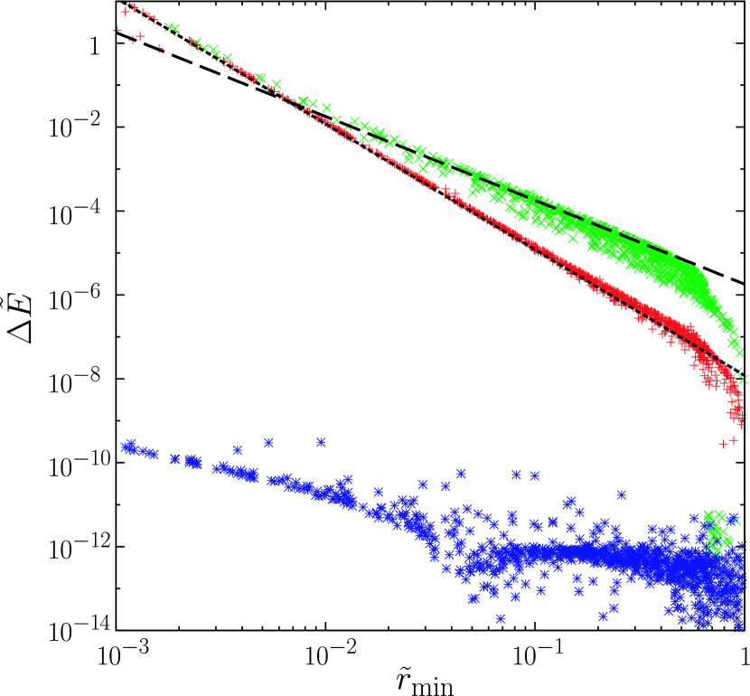
Figure 4: Total change of the energy $\tilde{E}$ due to gas drag through an encounter with the planet for each orbit, as a function of the minimum distance to the planet center in the case with $\alpha=3.113$. Red pluses and green crosses show the low-velocity ($\tilde{e}=3$) and high-velocity ($\tilde{e}=30$) cases, respectively. For each value of $\tilde{e}$, numerical results for $\xi=1\times 10^{-9}$ with a wide range of initial phase angle $\tau$ and impact parameter $\tilde{b}$ in the two-dimensional case ($\tilde{i}=0$) are shown. Blue asterisks show the case without gas drag, that is, the error of the numerical integration. Long-dashed line shows the approximate analytic results (Eq.(12)) for the high-velocity regime (i.e., the term proportional to $\tilde{r}_{\rm min}^{1-\alpha}$) and short-dashed line shows that for the low-velocity regime (the term proportional to $\tilde{r}_{\rm min}^{-\alpha}$). We set $f_{\rm c}=2$.

Figure 4 shows the total change of energy $\tilde{E}$ due to gas drag through an encounter with the planet until one of the truncation conditions for orbital integration (i)–(iii) is met, as a function of the minimum approach distance from the planet’s center. Two groups of points with $\Delta\tilde{E}\gtrsim 1\times 10^{-9}$ (red pluses and green crosses) show numerical results for the low- and high-velocity cases, respectively. We can see that the energy dissipation is well described by the analytic estimates given by Eq. (12), which are shown by the two lines (we set $f_{\rm c}=2$ in Eq.(12)). For the low velocity case, $\Delta\tilde{E}\propto\tilde{r}_{\rm min}^{-\alpha}$, which corresponds to the second term of Eq. (12) and means that the particles are well accelerated by the planet gravity at $\tilde{r}\sim\tilde{r}_{\rm min}$. For the high velocity case, $\Delta\tilde{E}\propto\tilde{r}_{\rm min}^{1-\alpha}$, which corresponds to the first term of Eq. (12) and means that the particle velocity around $\tilde{r}\sim\tilde{r}_{\rm min}$ is not much larger than $\tilde{v}_{\infty}$. We also plot the changes of $\tilde{E}$ for calculations without gas drag, which corresponds to the numerical error in our numerical integration. We find that the numerical error is much smaller than the calculated energy changes due to gas drag, even in the case when gas drag is very weak ($\xi=1\times 10^{-9}$).

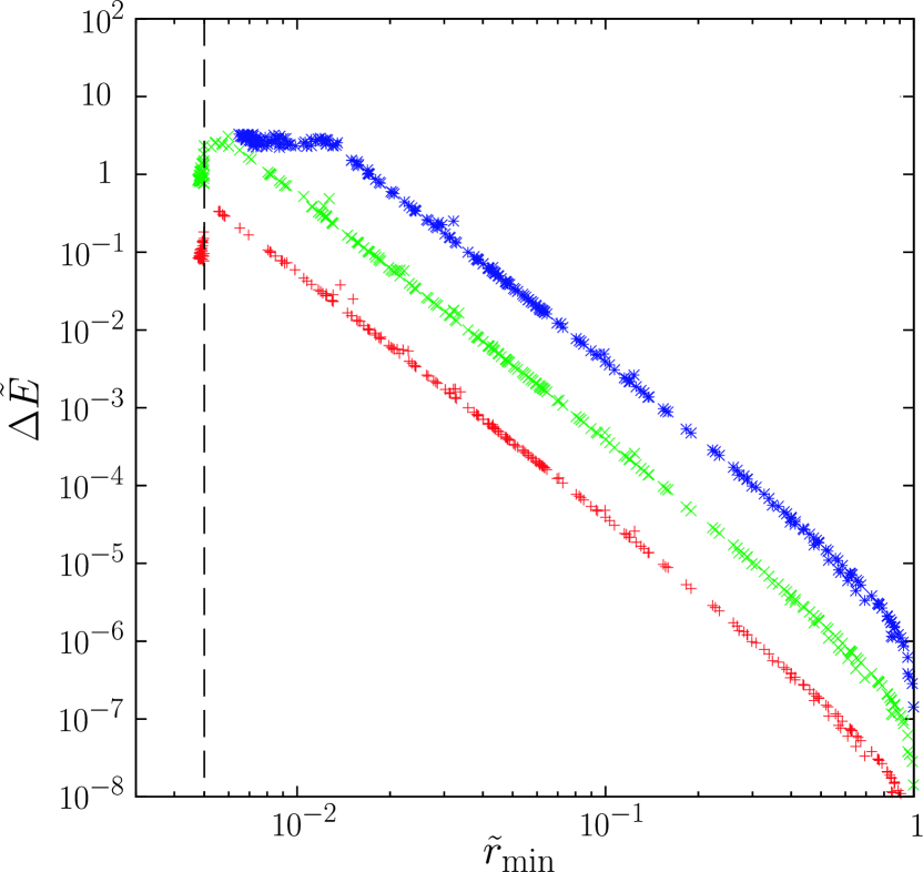
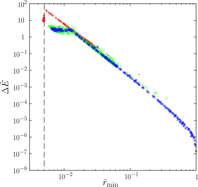
Figure 5: Total change of the energy $\tilde{E}$ due to gas drag through an encounter with the planet for each orbit, as a function of the minimum distance in the case with $\alpha=3.113$. Left panel shows the dependence on $\xi$ when $(\tilde{e},\tilde{i})=(0.1,0.05)$: red pluses, green crosses, and blue asterisks are the cases with $\xi=2.56\times 10^{-9}$ (weak), $2.56\times 10^{-8}$ (intermediate), and $2.56\times 10^{-7}$ (strong), respectively. Right panel shows the dependence on initial orbital elements when $\xi=2.56\times 10^{-7}$: red pluses, green crosses, and blue asterisks are the case with $(\tilde{e},\tilde{i})=(10,5)$, $(1,0.5)$, and $(0.1,0.05)$, respectively. The vertical dashed line shows the planet’s radius $\tilde{r}_{\rm p}=5\times 10^{-3}$.

In Fig. 5, we show the total change of $\tilde{E}$ in the same way as Fig. 4 in the case with $\tilde{r}_{\rm p}=0.005$ to examine the dependence on $\xi$ and $\tilde{e}$. Note that there are cases when the second or a later close approach reduces energy by an amount comparable to or larger than that due to the first one even when planetesimals are not captured within the Hill sphere yet, but such events are rare unless planetesimals are captured by the first close approach. Thus, the values of $\Delta\tilde{E}$ shown in Fig. 5 practically represent the energy change due to the first close approach to the planet, which can be used as an indicator whether planetesimals are captured or not from the point of view of energetics. The left panel shows the dependence on $\xi$ for a low-velocity case. In this cases, we find $\Delta\tilde{E}\propto\tilde{r}_{\rm min}^{-\alpha}$ for most points, as explained above. In the weak gas drag case, planetesimals reduce their energy due to single close encounter and escape from the Hill sphere. In the strong gas drag case, points shift upward in accordance with stronger energy dissipation. The points in this case fall on a horizontal band with $\Delta\tilde{E}\sim$ 2–3 at $\tilde{r}_{\rm min}\lesssim 0.015$; in this regime, particles are captured by gas drag rather than direct collision onto the planet, i.e., orbital integration is stopped by the condition $\tilde{E}<0$. Thus, values of $\Delta\tilde{E}$ in this horizontal band in the plot show the amount of energy that needs to be dissipated for capture, and the upper end of this horizontal band ($\tilde{r}_{\rm min}\sim 0.015$) corresponds to $\tilde{R}_{\rm c}$ (see Eq. (17)). When gas drag is weaker, energy dissipation becomes smaller and $\tilde{R}_{\rm c}$ becomes smaller accordingly, and eventually the trend $\Delta\tilde{E}\propto\tilde{r}_{\rm min}^{-\alpha}$ does not reach the energy needed to be captured ($\Delta\tilde{E}\sim$ 2–3 in this case) before it reaches the surface of the planet ($\tilde{r}=\tilde{r}_{\rm p}$); in this case, particles are accreted by direct collision. Note that the points with $\tilde{r}_{\rm min}\lesssim 0.005$ represent cases where orbital integrations were stopped by the condition of direct collision to the planet. The right panel shows the dependence on random velocity (i.e., $\tilde{e}$ and $\tilde{i}$). The low velocity case is identical to the strong drag case in the left panel. With increasing random velocity, the energy needed to be captured increases because initial kinetic energy is larger, and $\tilde{R}_{\rm c}$ decreases accordingly. In the high velocity case, the numerical results fall on a line with a nearly constant slope which extends all the way to $\tilde{r}_{\rm min}=\tilde{r}_{\rm p}$, which means that gas drag is not strong for particles with such a high random velocity and they are accreted only by direct collision with the planet’s solid surface.

3.3 Accretion rates for the case with $\tilde{e}=2\tilde{i}$

Next, we examine accretion rates in the case of $\tilde{e}=2\tilde{i}$. Figure 6 shows the plots of $p_{\rm col}(\tilde{e},\tilde{i},\tilde{b})$ and $p_{\rm cap}(\tilde{e},\tilde{i},\tilde{b})$ as a function of $\tilde{b}$, for two different sets of $(\tilde{e},\tilde{i})$. Crosses and pluses represent numerical results for $p_{\rm col}$ (Eq.(11)) and $p_{\rm cap}$ (Eq.(18)), respectively, and the dotted and solid lines show the analytic results. Note that we empirically set $f_{\rm c}=1.83$ for the analytic results of $p_{\rm cap}$; changing $f_{\rm c}$ only shifts the lines in the vertical direction and does not change the functional form. In the high $(\tilde{e},\tilde{i})$ case, we find that the numerical results are in good agreement with the analytic solutions over a wide range of $\tilde{b}$, except for the small-$\tilde{b}$ region where some small deviations are observed. In the low $(\tilde{e},\tilde{i})$ case, numerical results deviate from the analytic solution significantly. This is because $\tilde{v}_{\infty}$ is not large enough to neglect the three-body effect in this case.

Figure 7 shows numerical results of $P_{\rm acc}$ for several values of $\xi$, along with $P_{\rm col}$ (bottom line). We also plot numerical results for $P_{\rm col,Hill}$, which is the collision rate onto the Hill sphere (top line). All these curves can be roughly divided into two parts: a horizontal part in the low-velocity regime and a part with a negative slope in the high-velocity regime. In the lower eccentricity regime, previous studies showed that $P_{\rm col}$ is independent of $\tilde{v}_{\infty}$ and depends on $\tilde{r}_{\rm p}$ as (Ida and Nakazawa, 1989; Inaba et al., 2001)

$$P_{\rm col,low}=11.3\sqrt{\tilde{r}_{\rm p}}.$$ (19)

This corresponds to the horizontal part of the curve for $P_{\rm col}$ in Fig. 7, even though the horizontal part can be seen only in the lowest $\tilde{e}$ regime displayed in the left figure. In the high eccentricity regime, $P_{\rm col}$ can be well described by Eq. (10) and is thus proportional to $\tilde{e}^{-2}$; this corresponds to the negative-slope part of the above curve.

In the case for planets with atmospheres, this general trend still holds, but changes in some parts. In the lower eccentricity regime, $P_{\rm cap}$ is expected to be proportional to $\xi^{1/2\alpha}$, because $P_{\rm cap}\propto\tilde{R}_{\rm c}^{1/2}$ (see Eq. (19)) and $\tilde{R}_{\rm c}\simeq(4f_{\rm c}\xi/3)^{1/\alpha}$ (see Eq. (17)). On the other hand, Fig. 7 shows a rather weak dependence on $\xi$ in the low-velocity regime, especially when $\xi\geq 10^{-5}$. In order to examine the $\xi$-dependence in the low-velocity regime in detail, we calculated capture rates as a function of $\xi$ for $\tilde{e}=\tilde{i}=0$ (Fig. 8). In the low $\xi$ regime ($\xi\lesssim 10^{-5}$ when $\alpha=3$), $P_{\rm cap}$ is indeed $\propto\xi^{1/2\alpha}$. In the high $\xi$ regime ($\xi>1$), on the other hand, $P_{\rm cap}$ is constant and is equal to the collision rate onto the Hill sphere, because particles entering the Hill sphere immediately get captured due to the strong gas drag. In between the above two extreme regimes of $\xi$ in Fig. 8, there is a part where $P_{\rm cap}$ is well approximated by $\xi^{1/10\alpha}$ at $10^{-5}\lesssim\xi\lesssim 1$ when $\alpha=3$. We thus obtain the following empirical formula for capture rates in the low velocity regime

$$P_{\rm cap0}=\min(P_{\rm cap0,low\xi},P_{\rm cap0,med\xi},P_{\rm col0,Hill}),$$ (20)

where $P_{\rm cap0,low\xi}$ is the capture rate in the low $\xi$ regime, $P_{\rm cap0,med\xi}$ is the one for the intermediate $\xi$ regime, and $P_{\rm col0,Hill}$ is the collision rate onto the Hill sphere, respectively, and these variables are defined in the case with $\tilde{e}=\tilde{i}=0$, given by

$$P_{\rm cap0,low\xi}=10.7\left(\frac{{\xi}}{{0.082}}\right)^{1/2\alpha},$$ (21)

$$P_{\rm cap0,med\xi}=P_{\rm col,Hill}\xi^{1/10\alpha},$$ (22)

$$P_{\rm col0,Hill}=4.392.$$ (23)

As we can see in Fig. 8, the expressions (20)–(23) reproduce our numerical results very well, even when $\alpha=2$ and 4.

In the high-velocity regime, we can see from Fig. 7 that, when $\tilde{e}\sim 10$ and $\xi$ is small, the $\tilde{e}$-dependence of $P_{\rm cap}$ is stronger than that of $P_{\rm col}$ ($\propto\tilde{e}^{-2}$), because $\tilde{R}_{\rm c}$ decreases with increasing random velocity in this regime (see Eq. (17)). Thus, with increasing $\tilde{e}$, $P_{\rm acc}$ for small $\xi$ approaches $P_{\rm col}$ at a certain $\tilde{e}$ ($\tilde{e}\sim 5$ when $\xi=10^{-7}$ and $\tilde{r}_{\rm p}=0.005$, for example). In §4, we will derive an analytic expression of the capture rate in this regime. The expression shows that the capture rate is expected to be proportional to $\tilde{e}^{-8/3}$ when $\alpha=3$ and $\tilde{e}=2\tilde{i}$, which agrees well with the above numerical results.

3.4 Accretion rates averaged over the distribution of eccentricities and inclinations

Planetesimals in protoplanetary disks have a distribution of eccentricities and inclinations that is well described by the Rayleigh distribution function (Ida and Makino, 1992), thus we next show $P_{\rm acc}$ for incoming planetesimals that have the Rayleigh distribution in eccentricity and inclination.

Normalized accretion rate for planetesimals that have a Rayleigh distribution in $\tilde{e}$ and $\tilde{i}$ with the root mean square values $\tilde{e}^{\ast}$ and $\tilde{i}^{\ast}$ is given by

$$\langle P_{\rm acc}\rangle\equiv\iint P_{\rm acc}f_{\rm R}(\tilde{e},\tilde{i},\tilde{e}^{\ast},\tilde{i}^{\ast})d\tilde{e}d\tilde{i},$$ (24)

where $f_{\rm R}$ is the Rayleigh distribution function given by

$$f_{\rm R}(\tilde{e},\tilde{i},\tilde{e}^{\ast},\tilde{i}^{\ast})=\frac{4\tilde{e}\tilde{i}}{(\tilde{e}^{\ast})^{2}(\tilde{i}^{\ast})^{2}}\exp\left(-\frac{\tilde{e}^{2}}{(\tilde{e}^{\ast})^{2}}-\frac{\tilde{i}^{2}}{(\tilde{i}^{\ast})^{2}}\right).$$ (25)

In order to obtain $\langle P_{\rm acc}\rangle$ from Eq. (24) for certain regimes of $\tilde{e}^{\ast}$ and $\tilde{i}^{\ast}$ ($10^{-1}\leq\tilde{e}^{\ast}\leq 10^{5/4}$ and $10^{-1}\leq\tilde{i}^{\ast}\leq 10^{5/4}$ in this paper), we need values of $P_{\rm acc}$ for a wide range of $\tilde{e}$ and $\tilde{i}$ including the region outside of the regime of $\tilde{e}^{\ast}$ and $\tilde{i}^{\ast}$ (Ohtsuki, 1999). To do that, we follow the method described in Ohtsuki (1999) with a slight modification.

We first obtain $P_{\rm acc}(\tilde{e},\tilde{i})$ by direct orbital integration described in the previous sections at the $10\times 10$ mesh points in the square region $10^{-1}\leq\tilde{e}\leq 10^{5/4}$ and $10^{-1}\leq\tilde{i}\leq 10^{5/4}$ with even interval in the logarithmic space. We also perform orbital integration at supplementary coarse grid points in the low inclination regime, i.e., $3\times 2$ mesh points with $\tilde{e}=10^{-1},10^{0},10^{1}$ and $\tilde{i}=10^{-3},10^{-2}$. Values outside of the region are obtained by extrapolation from the calculated region and by the analytic estimation for the high-velocity regime (see §4). We confirmed that $\langle P_{\rm acc}\rangle$ for $10^{-1}\leq\tilde{e}^{\ast}\leq 10^{5/4}$ does not depend sensitively on the $P_{\rm acc}$ values for the outside of the square region $10^{-1}\leq\tilde{e}\leq 10^{5/4}$ and $10^{-1}\leq\tilde{i}\leq 10^{5/4}$.

Symbols in Fig. 9 shows numerical results for $\langle P_{\rm acc}\rangle$ as a function of $\tilde{e}^{\ast}$ when $\tilde{e}^{\ast}=2\tilde{i}^{\ast}$. While this figure looks similar to Fig. 7, the results shown in Fig. 9 change more smoothly with increasing random velocity than those of Fig. 7, and the absolute values in Fig. 9 tend to be slightly higher than those of Fig. 7 in the high-velocity regime. These two differences come from the average over the Rayleigh distribution, and similar results were obtained for the Rayleigh distribution average of collision rates (Greenzweig and Lissauer, 1992).

4 A semi-analytic expression for accretion rates

Next, we derive a semi-analytical expression for $\langle P_{\rm acc}\rangle$ based on the numerical and analytical calculations for accretion rates described above. As shown in Figs. 7 and 9, with decreasing strength of gas drag (i.e., $\xi$), accretion rates decrease and approach the collision rates onto the solid surface of the planet without an atmosphere. Thus $\langle P_{\rm acc}\rangle$ can be approximated by the larger of $\langle P_{\rm col}\rangle$ and $\langle P_{\rm cap}\rangle$:

$$\langle P_{\rm acc}\rangle(\tilde{r}_{\rm p},\xi,\alpha,\tilde{e}^{\ast},\tilde{i}^{\ast})=\max(\langle P_{\rm col}\rangle(\tilde{r}_{\rm p},\tilde{e}^{\ast},\tilde{i}^{\ast}),\langle P_{\rm cap}\rangle(\xi,\alpha,\tilde{e}^{\ast},\tilde{i}^{\ast})).$$ (26)

Collision rate averaged over the Rayleigh distribution was studied in detail by previous work (e.g., Greenzweig and Lissauer, 1992), and Inaba et al. (2001) derived the following semi-analytic expression for $\langle P_{\rm col}\rangle$:

$$\langle P_{\rm col}\rangle=\min\left(\langle P_{\rm col}\rangle_{\rm med},\left\{\langle P_{\rm col}\rangle_{\rm low}^{-2}+\langle P_{\rm col}\rangle_{\rm high}^{-2}\right\}^{-1/2}\right),$$ (27)

where

$$\langle P_{\rm col}\rangle_{\rm low}=11.3\sqrt{\tilde{r}_{\rm p}},$$ (28)

$$\langle P_{\rm col}\rangle_{\rm med}=\frac{\tilde{r}_{\rm p}^{2}}{4\pi\tilde{i}^{\ast}}\left(17.3+\frac{232}{\tilde{r}_{\rm p}}\right),$$ (29)

$$\langle P_{\rm col}\rangle_{\rm high}=\frac{\tilde{r}_{\rm p}^{2}}{2\pi}\left({\cal F}(I^{\ast})+\frac{6}{\tilde{r}_{\rm p}}\frac{{\cal G}(I^{\ast})}{(\tilde{e}^{\ast})^{2}}\right).$$ (30)

In the above, Eq.(30) was obtained by averaging Eq. (10) over the Rayleigh distribution (Greenzweig and Lissauer, 1992); $I^{\ast}\equiv\tilde{i}^{\ast}/\tilde{e}^{\ast}$ and the function ${\cal F}(I^{\ast})$ and ${\cal G}(I^{\ast})$ are given by

$${\cal F}(I^{\ast})\equiv 8\int_{0}^{1}d\lambda\frac{(I^{\ast})^{2}E[\sqrt{3(1-\lambda^{2})}/2]}{[(I^{\ast})^{2}+(1-(I^{\ast})^{2})\lambda^{2}]^{2}},$$ (31)

$${\cal G}(I^{\ast})\equiv 8\int_{0}^{1}d\lambda\frac{K[\sqrt{3(1-\lambda^{2})}/2]}{[(I^{\ast})^{2}+(1-(I^{\ast})^{2})\lambda^{2}]}.$$ (32)

When $I^{\ast}=1/2$, ${\cal F}(1/2)=17.34$ and ${\cal G}(1/2)=38.22$.

As for the capture rate averaged over the Rayleigh distribution, we found that the following expression reproduces our numerical results very well:

$$\langle P_{\rm cap}\rangle=\left(\langle P_{\rm cap}\rangle_{\rm low}^{-\eta}+\langle P_{\rm cap}\rangle_{\rm high}^{-\eta}\right)^{-1/\eta},$$ (33)

with $\eta=2/3$. The accretion rate for the low-velocity regime can be simply written in terms of $P_{\rm cap0}$ (Eq.(20)) as

$$\langle P_{\rm cap}\rangle_{\rm low}=P_{\rm cap0},$$ (34)

because $P_{\rm cap0}$ is independent of $\tilde{e}$ and $\tilde{i}$. We further divide $\langle P_{\rm cap}\rangle_{\rm high}$ into two functions as

$$\langle P_{\rm cap}\rangle_{\rm high}=\langle P_{\rm cap}\rangle_{\rm high1}+\langle P_{\rm cap}\rangle_{\rm high2}.$$ (35)

We define that $\langle P_{\rm cap}\rangle_{\rm high1}$ is for a relatively low-velocity regime in the sense that the relative velocity is low enough for the collision cross-section to be enhanced by gravitational focusing, whereas it is still high enough to hold the two-body approximation. On the other hand, $\langle P_{\rm cap}\rangle_{\rm high2}$ is defined for a higher velocity regime where gravitational focusing is negligible. In the former regime, $P_{\rm cap,high1}$ can be obtained by the integration of Eq. (18) as in Eq. (8):

$$P_{\rm cap,high1}=\frac{12(12f_{\rm c}\xi)^{1/\alpha}}{\pi\tilde{i}(\tilde{e}^{2}+\tilde{i}^{2})^{\gamma}}R(k,\gamma),$$ (36)

where $\gamma\equiv(\alpha+2)/2\alpha$, and $R(k,\gamma)$ is an integral similar to the complete elliptic integral, and is defined by

$$R(k,\gamma)\equiv\int_{0}^{1}\frac{dx}{(1-x^{2})^{1/2}(1-k^{2}x^{2})^{\gamma}}.$$ (37)

The Rayleigh distribution average of $P_{\rm cap,high1}$ can be calculated as

$$\langle P_{\rm cap}\rangle_{\rm high1}\simeq\frac{24(12f_{\rm c}\xi)^{1/\alpha}R(k,\gamma)}{\pi(\tilde{e}^{\ast})^{2\gamma-1}(\tilde{i}^{\ast})^{2}}\Gamma\left(\frac{3}{2}-\gamma\right){{}_{2}F_{1}}\left(\frac{1}{2},\frac{3}{2}-\gamma,\frac{3}{2},1-\frac{(\tilde{e}^{\ast})^{2}}{(\tilde{i}^{\ast})^{2}}\right),$$ (38)

where $\Gamma$ is the gamma function, ${}_{2}F_{1}$ is the hypergeometric function, and we assume $\tilde{e}^{\ast}>\tilde{i}^{\ast}$ and $\alpha>1$. This gives $\langle P_{\rm cap}\rangle_{\rm high1}\propto(\tilde{e}^{\ast})^{-(2\gamma+1)}=(\tilde{e}^{\ast})^{-2(\alpha+1)/\alpha}$ when $\tilde{e}^{\ast}=2\tilde{i}^{\ast}$, whose dependence on $\tilde{e}^{\ast}$ (i.e., $\propto(\tilde{e}^{\ast})^{-2(\alpha+1)/\alpha}$) agrees with that of $P_{\rm cap,high1}$ on $\tilde{e}$ when $\tilde{e}=2\tilde{i}$. For the typical case of $\alpha=3$ and $\tilde{e}^{\ast}=2\tilde{i}^{\ast}$, we have $\langle P_{\rm cap}\rangle_{\rm high1}\simeq 1.52\times 10^{2}(f_{\rm c}\xi)^{1/3}(\tilde{e}^{\ast})^{-8/3}$. In deriving Eq. (38), we treated $R(k,\gamma)$ as a constant, because $R(k,\gamma)$ is a slowly varying function of $k$ as long as $k$ is not close to unity (note that $0\leq k\leq\sqrt{3/4}$ from its definition). For the still higher velocity regime,

$$P_{\rm cap,high2}=\frac{2(2f_{\rm c}\xi)^{2/(\alpha-1)}}{\pi}\sqrt{(\tilde{e}/\tilde{i})^{2}+1}E(k),$$ (39)

thus

$$\langle P_{\rm cap}\rangle_{\rm high2}=\frac{(2f_{\rm c}\xi)^{2/(\alpha-1)}}{2\pi}{\cal F}(I^{\ast}).$$ (40)

The curves in Fig. 9 show $\langle P_{\rm acc}\rangle(\tilde{r}_{\rm p},\xi,\alpha,\tilde{e}^{\ast},\tilde{i}^{\ast})$ obtained using the above semi-analytic expressions. We can see that $\langle P_{\rm acc}\rangle$ is well approximated by the above semi-analytical expressions within a factor of two for the entire regions of random velocity and $\xi$. When $\tilde{r}_{\rm p}$ is large, $\langle P_{\rm acc}\rangle$ tends to approach $\langle P_{\rm col}\rangle$ because planetesimals tend to collide with the planet more easily before losing a sufficient amount of energy by gas drag to get captured. For example, when $\tilde{r}_{\rm p}=0.005$ (left panel) and $\xi=10^{-9}$, $\langle P_{\rm acc}\rangle=\langle P_{\rm col}\rangle$, which can be deduced by Fig. 1. On the other hand, $\langle P_{\rm acc}\rangle$ can be approximated by $\langle P_{\rm cap}\rangle$ when $\xi$ is large. In summary, the effect of atmosphere is statistically negligible in the entire velocity regime when $\xi$ is so small that $\langle P_{\rm col}\rangle_{\rm high}>\langle P_{\rm cap}\rangle_{\rm high1}$ is satisfied, where $\langle P_{\rm col}\rangle_{\rm high}$ and $\langle P_{\rm cap}\rangle_{\rm high1}$ are given by Eqs.(30) and (38), respectively. This condition can be written in terms of $\xi$ as

$$\xi<4\times 10^{-9}\left(\frac{{\tilde{r}_{\rm p}}}{{0.005}}\right)^{3}.$$ (41)

To derive the condition, we set $\tilde{e}^{\ast}=2$ as the lowest limit of the range for the functions.

It should be noted that when the mass of planetesimals are small ($\lesssim 10^{14}$g), the assumption of $\tilde{e}^{\ast}=2\tilde{i}^{\ast}$ breaks down if protoplanetary gas disk still exists and runaway bodies significantly perturb the orbit of such small bodies (Ohtsuki et al., 2002). This is because, once inclination is damped to $\tilde{i}\leq 1$, the stirring rate of inclination by the large bodies is much smaller than that of eccentricity in such a velocity regime, and only eccentricity tends to be enhanced (Ida, 1990).

Using analytic calculation of planetesimals’ energy dissipation due to gas drag under the two-body approximation neglecting the solar gravity, Inaba and Ikoma (2003) derived a relation between the size of planetesimals and the enhanced radius of protoplanets, for a given atmospheric structure (their Eq.(17)). Substituting this enhanced radius for the planetary radius in the expressions for collision rates derived by Inaba et al. (2001), semi-analytic expressions of accretion rates for protoplanets with atmospheres can be obtained (Inaba and Ikoma, 2003, their Eqs.(20)-(24)). We find that $\langle P_{\rm acc}\rangle$ with the effect of atmospheric gas drag obtained from these expressions derived by Inaba and Ikoma (2003) ($\langle P_{\rm col}\rangle$ in their notation) is smaller by a factor of about two as compared to ours in the high-velocity regime, even when the same atmospheric structure is assumed (Fig.10). This discrepancy is caused by the more simplified procedures in deriving the expression in Inaba and Ikoma (2003) as compared to ours; the cause for the discrepancy is further discussed in detail in Appendix B. On the other hand, Inaba and Ikoma (2003) obtained the enhanced radius using more realistic atmospheric structures, while we assumed a power-law density distribution. Effects of this assumption will be discussed in Section 5.

5 Comparison with the case of more realistic atmospheric structures

Here, we examine the validity of our assumption of the simplified atmospheric structure, i.e., power-law function (Eq.(4)). As shown above, the assumption of power-law approximation for gas density in atmospheres allowed a systematic study and understanding of the dependence of the accretion rate on various physical parameters. In order to check the validity of this assumption, we compared the results shown previously in this paper with those obtained using a more realistic atmospheric structure based on the analytic solution shown by Inaba and Ikoma (2003). Although the index $\alpha$ should be properly chosen depending on the parameter values for a given atmospheric structure, we found that the use of power law functions is a good approximation in most cases to describe realistic atmospheres when opacity depletion factor $f_{\kappa}$ is much smaller than unity ($f_{\kappa}\lesssim 10^{-2}$), because optically thin atmospheres tend to be radiative rather than convective. The assumption of small $f_{\kappa}$ would be reasonable, because a large fraction of dust in protoplanetary disks in this stage would be depleted after the accretion of large bodies such as planetesimals or protoplanets. In addition, small $f_{\kappa}$ also corresponds to the situation when dust size is much larger than sub-micron size, and this would be the case for large protoplanets ($M\gtrsim M_{\oplus}$), because dust in the atmospheres grows quickly to reduce opacity by a factor of 100 from that of sub-micron size dust (Movshovitz and Podolak, 2008).

However, the power-law distribution would not be a good approximation at outer region of the atmospheres in some cases. The density profile fitted by a power-law function at the bottom of an atmosphere tends to underestimate the gas density at the outer region when planet mass is small ($M\sim 0.1M_{\oplus}$) and overestimate it when planet mass is large ($M\sim 10M_{\oplus}$) for typical disk parameters. In the case of small planets, however, the atmosphere is not very effective in capturing planetesimals because it is not massive enough. On the other hand, the effect of atmospheric gas drag on accretion rates is most important for such large bodies as $M\sim 10M_{\oplus}$, because they have thick and massive atmospheres (Inaba and Ikoma, 2003). Also, the formation timescale of protoplanets is determined by the later stage of accretion (i.e., when $M\sim$ 1–10$M_{\oplus}$ for $\sim$ 5AU) where their growth timescale is long. Thus here we concentrate on the cases of large protoplanets, and compare accretion rates for atmospheres with power-law density profiles and those for more realistic atmospheric structures. As examples, we consider cases of $1M_{\oplus}$ and $10M_{\oplus}$ planets at 5AU when disk gas temperature is 125K and density is $1.5\times 10^{-8}{\rm kg\,m^{-3}}$. We set the density of solid part of the planets to be $3.4\times 10^{3}{\rm kg\,m^{-3}}$ ($\tilde{r}_{\rm p}=0.001$), which represents the density of $10M_{\oplus}$ planets that consist of ice and rock for roughly even mass (e.g., Fortney et al., 2007).

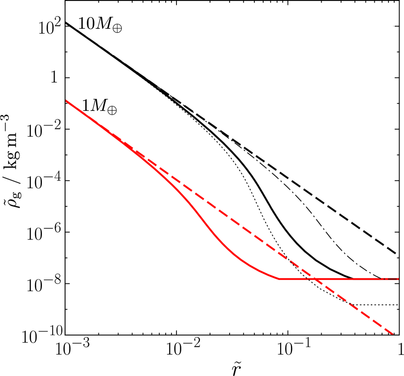
Figure 11: Density profiles of a realistic atmosphere derived by the analytic method given in Inaba and Ikoma (2003) for $1M_{\oplus}$ and $10M_{\oplus}$ planets at 5AU (thick-solid lines) in the case when $\rho_{\rm core}=3.4\times 10^{3}{\rm kg\,m^{-3}}$, $L=10^{-7}L_{\odot}$, and $f_{\kappa}=10^{-2}$, and power-law functions fitted to the realistic one at the bottom (thick-dashed lines). The exponents for the fit lines are $\alpha=3.094$ for $1M_{\oplus}$ and $\alpha=3.027$ for $10M_{\oplus}$. Thick lines show the case when the temperature and gas density at the outer boundary are 125K and $1.5\times 10^{-8}{\rm kg\,m}^{-3}$, respectively. In order to see the dependence on the boundary condition, we also show density profiles when the temperature at the boundary is lower (50K, thin dot-dashed line) and the density is lower ($1.5\times 10^{-9}{\rm kg\,m^{-3}}$, thin dotted line) in the $10M_{\oplus}$ case.

Figure 11 shows the density profiles derived by the method given by Inaba and Ikoma (2003) together with fitted power-law profiles. As we can see, the fitted power-law functions overestimate the gas density in the outer region $(\tilde{r}\gtrsim 0.01)$, by a factor of up to $\sim 10^{2}$ for the $10M_{\oplus}$ case. As for the $1M_{\oplus}$ case, the line for the power-law distribution crosses the realistic one and underestimates the gas density at the outermost region $(\tilde{r}>0.2)$ because the region is already outside of the outer boundary of the analytic solution given by Inaba and Ikoma (2003) and the temperature and density are constant. The density profile at the outer region also depends on the outer boundary condition, which will be briefly discussed later in this section.

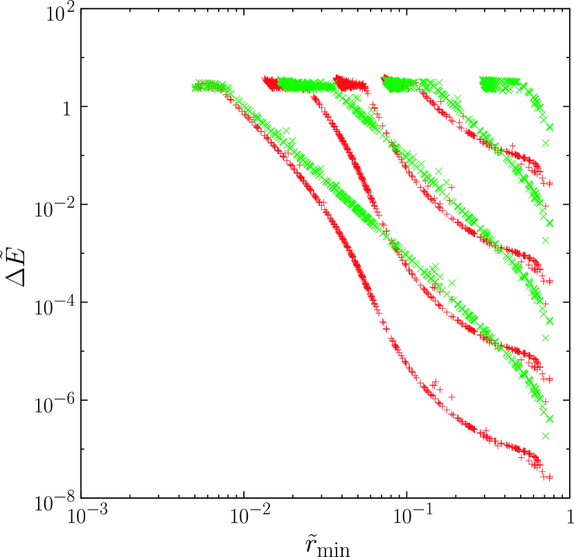
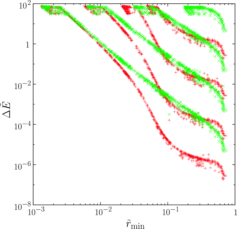
Figure 12: Change of the energy $\tilde{E}$ due to gas drag as a function of minimum approach distance (the same as Fig. 5) for a realistic atmosphere model (red pluses) and a power-law model (green crosses) when $M=10M_{\oplus}$ at 5AU. Left and right panels show the case when $(\tilde{e},\tilde{i})=(0.1,0.05)$ and $(10,5)$, respectively. Four different planetesimal sizes are assumed for each of the two atmosphere models; $r_{\rm s}=10^{4}$km, $10^{2}$km, 1km, and 10m, from lower-left to upper-right.

Figure 12 shows $\Delta\tilde{E}$ obtained by orbital integration as a function of $\tilde{r}_{\rm min}$ for the two density profiles for the $10M_{\oplus}$ planet for various planetesimal sizes ($10$ – $10^{7}$m) with $\tilde{e}=0.1$ and 10 in order to examine the dependence of $\tilde{R}_{\rm c}$ on $r_{\rm s}$ (or $\xi$) and $\tilde{e}$ when $\tilde{e}=2\tilde{i}$ (the values of $\tilde{r}_{\rm min}$ for the upper end of the horizontal band for each curve in this plot corresponds to $\tilde{R}_{\rm c}$, as we discussed in §3.2). In the case of $\tilde{e}=0.1$ (left panel), we can see from the shapes of the curves that the difference of $\Delta\tilde{E}$ directly reflects the assumed density profiles (Fig. 11). When planetesimals are large ($r_{\rm s}=10^{4}$km), $\tilde{R}_{\rm c}$ of the two atmospheres are almost the same because the two curves eventually agree where the curves reach $\Delta\tilde{E}\sim 2-3$, which is necessary to be captured within the Hill sphere when $\tilde{e}\sim 0.1$. But as planetesimals become smaller, the curves of $\Delta\tilde{E}$, which is dissipation energy per unit mass, shift upward, which yields two different $\tilde{R}_{\rm c}$, the values for the realistic atmospheric model being smaller. When $r_{\rm s}=$1km, the difference in the value of $\tilde{R}_{\rm c}$ for the two atmospheric profiles is about a factor of three. In the case of $\tilde{e}=10$ (right panel), energy dissipation required for capture is larger. Thus, in order to be captured, planetesimals have to pass through the inner dense region of the atmosphere, where the difference of the two density profiles are smaller, yielding better agreement in $\tilde{R}_{\rm c}$ for $\tilde{r}_{\rm s}\geq 1$km.

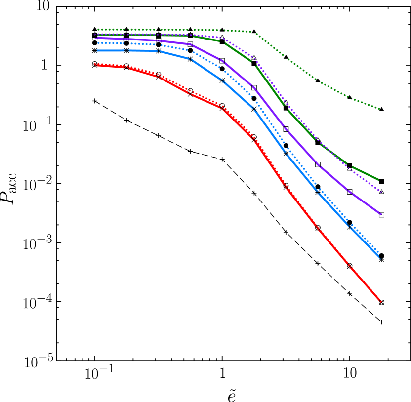
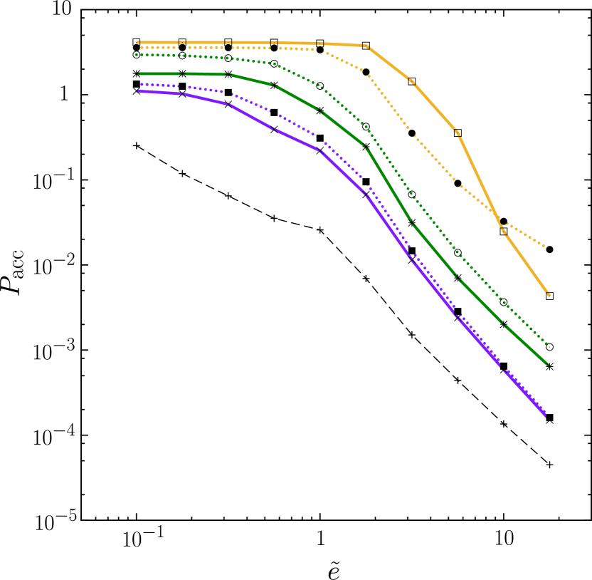
Figure 13: $P_{\rm acc}$ for the realistic atmosphere model (thick-solid lines) and for the power-law atmosphere model (thick-dotted lines), and $P_{\rm col}$ for $\tilde{r}_{\rm p}=0.001$ (thin dashed line) ($\tilde{e}=2\tilde{i}$). Left panel shows the cases when $M=10M_{\oplus}$ with $r_{\rm s}=10^{4}$km (red lines), $10^{2}$km (blue lines), 1km (purple lines), and 10m (green lines). Right panel shows the cases when $M=1M_{\oplus}$ with $r_{\rm s}=$1km (purple lines), 10m (green lines), and 0.1m (yellow lines).

Figure 13 shows the plots of $P_{\rm acc}$ in the case of $\tilde{e}=2\tilde{i}$ for the two atmospheres for various planetesimal sizes. In the case of $M=10M_{\oplus}$ (left panel), $P_{\rm acc}$ for the fitted power-law density profile overestimates the accretion rate for small planetesimal sizes, as easily deduced from the results of Figs. 11 or 12, whereas the two values of $P_{\rm acc}$ for the two atmospheric models are almost the same when planetesimals are large. Smaller planetesimal cases tend to give a larger difference in $P_{\rm acc}$ because planetesimals are captured at outer atmospheres, where the difference of the two density profiles is larger. The values of $P_{\rm acc}$ differ by a factor of 2–3 for 1km planetesimals, and the difference is about a factor of 15 for 10m planetesimals. As for the dependence on eccentricity, there are two effects that shift $P_{\rm acc}$ in opposite directions. One is the $\tilde{e}$-dependence of the amount of energy dissipation required for capture, which we already discussed above and the difference in $P_{\rm acc}$ for the two atmospheric profiles becomes smaller for planetesimals with higher eccentricities (Fig. 12). This tendency can be seen in the case of $r_{\rm s}=10^{2}$km, where the difference between the results for the two atmospheric profiles becomes smaller with increasing $\tilde{e}$. The other is the effect of gravitational focusing by the planet. When the initial random velocity of incoming planetesimals is small ($\tilde{e}\lesssim 1$), velocities of planetesimals at $\tilde{R}_{\rm c}$ ($\ll 1$) are determined by the planet’s gravity, and thus the effective collision cross section is proportional to $\tilde{R}_{\rm c}$ (cf. Eq. (18)). Therefore, the difference in $P_{\rm acc}$ is roughly proportional to the difference of $\tilde{R}_{\rm c}$. However, when the initial random velocity is large, planetesimals are not significantly accelerated by the planet’s gravity at locations with $\tilde{r}\gtrsim 6/\tilde{e}^{2}$. Thus, when $\tilde{R}_{\rm c}\gtrsim 6/\tilde{e}^{2}$, $P_{\rm acc}$ tends to be proportional to the geometrical cross section, i.e., $\propto\tilde{R}_{\rm c}^{2}$, which amplifies the difference in $P_{\rm acc}$. This tendency can be seen in the case of $r_{\rm s}=10$m, where the difference between the results for the two atmospheric profiles becomes larger with increasing $\tilde{e}$. In the case of $M=1M_{\oplus}$, the difference between the values of $P_{\rm acc}$ for the two atmospheric profiles can be explained basically in a similar way. In both $1M_{\oplus}$ and $10M_{\oplus}$ cases, the difference between the results for the atmospheric profiles is rather small in the low-velocity regime with $\tilde{e}\leq 1$. One difference from the $M=10M_{\oplus}$ case is that $P_{\rm acc}$ with the power-law model for the smallest planetesimal case ($r_{\rm s}=0.1$m) underestimates the accretion rate when $\tilde{e}\lesssim 10$, which simply reflects the underestimation of the density at the outer region (see Fig. 11). However, it should be noted that the assumption of our numerical method (i.e., planetesimals move on a Keplerian orbit while weakly perturbed by gas drag) breaks down for such small planetesimals. Their motion is expected to be strongly coupled with the gas flow, and the accretion rate of such small planetesimals is determined by the flow pattern of the nebular gas in the vicinity of a planet, rather than the structure of the atmosphere near the planet’s surface. Therefore, the difference in the accretion rates for the two atmospheric profiles is practically negligible in the $M=1M_{\oplus}$ case, if we take into account the fact that sufficiently small planetesimals are coupled with the gas drag flow.

In summary, the power-law atmospheric density profile is a reasonable approximation for accretion rates of large ($\sim 10M_{\oplus}$) protoplanets when planetesimals’ size is not too small. In the case of $1M_{\oplus}$, the difference of the two atmospheric profiles practically does not cause a significant difference in $P_{\rm acc}$, if we take account of the fact that the motion of planetesimals with very small sizes ($\lesssim$ 0.1m) are strongly coupled with the nebular gas.

We further note that the outer boundary condition of atmospheres is important for the structure of the outer region of atmospheres, where the difference between realistic density profiles and fitted power-law profiles can be significant, although the inner dense region, which account for most of the atmospheric mass, is insensitive to the boundary condition. For example, when the temperature of the outer boundary is decreased to 50K, which is a typical disk temperature at 5AU for a disk that is optically thin in the vertical direction and optically thick in the horizontal direction, the agreement between the realistic density profile and the fitted power-law function is significantly improved (see Fig. 11); in this case, the difference in accretion rates for the two atmospheric profiles is expected to be reduced greatly. Conversely, when the density at the outer boundary decreases due to the dispersal of the nebular gas, for example, the difference between the two profile increases (Fig. 11).

6 Growth rates of protoplanets

In order to examine the consequence of the obtained formula of accretion rates, we calculate the time evolution of planet mass using a simple semi-analytic model with the accretion rate obtained above. We basically follow the calculation model of Chambers (2006a), and also compare our results with his results.

We consider a protoplanet embedded in a disk of single-size planetesimals, whose random velocity is determined by the equilibrium between damping by gas drag and excitation by the protoplanet. The growth rate of a protoplanet is given by

$$\frac{dM}{dt}=\left(\frac{2\pi\Sigma_{\rm p}r_{\rm H}^{2}}{T}\right)\langle P_{\rm acc}\rangle,$$ (42)

where $\Sigma_{\rm p}$ is the surface density of planetesimals and $T$ is the orbital period of the protoplanet. To integrate this equation, we need formulas for the surface density and $\langle P_{\rm acc}\rangle$. The surface density is given by

$$\Sigma_{\rm p}=\Sigma_{\rm tot}-\frac{M}{2\pi a\tilde{b}r_{\rm H}},$$ (43)

where $\Sigma_{\rm tot}$ is the initial surface density of planetesimals. This expression was derived under the assumption that the protoplanet does not migrate radially. In this case, the final mass of the planet becomes the isolation mass, $(2\pi a^{2}\tilde{b}_{\rm f}\Sigma_{\rm tot})^{3/2}/(3M_{\ast})^{1/2}$, where $\tilde{b}_{\rm f}$ is the width of the feeding zone of the planet scaled by the Hill radius. As for the normalized accretion rate, we use our semi-analytic expression for the high-velocity regime (Eq.(38)) in accordance with Chambers (2006a), who used the expression based on Inaba and Ikoma (2003) for the same velocity regime. Equation (38) includes the gas drag parameter $\xi$, which is a function of the accretion rate (see Eq.(7)). Thus we solve simultaneous equations with respect to $dM/dt$ (Eq.(42) with Eq.(38)) and $\xi$ self-consistently. We set $\Sigma_{\rm tot}=100\,{\rm kg\,m^{-2}}$ and $a=5$AU, and also assume that mean molecular weight is 2.8, material density is $2.0\times 10^{3}\,{\rm kg\,m^{-3}}$, gas density of the disk is $3.9\times 10^{-8}{\rm kg\,m^{-3}}$, opacity is $1.0\times 10^{-3}{\rm m^{2}\,kg^{-1}}$, and $\alpha=3$ for the atmospheric gas density distribution.

Figure 14(a) shows the growth of the protoplanet. We first calculated the growth with the formula used in Chambers (2006a) to check our calculation, and confirmed that their results in the case of planetesimals with 10km diameter can be reproduced (thin dashed line in Fig. 14(a); see also Fig.8 of Chambers (2006a)). As demonstrated by the semi-analytic calculation of Chambers (2006a), acceleration of the growth of protoplanets by the effect of atmospheric gas drag becomes notable when $M>M_{\oplus}$, because at this stage the atmospheres of the protoplanets become dense enough to capture 10-km-diameter planetesimals by gas drag.

On the other hand, the three thick lines in Fig. 14(a) show results obtained using our new formula for accretion rates with the effect of atmospheric gas drag. We also plot the change of values of $\xi$ in the course of planetary growth in these three cases in Fig. 14(b). We can see that the growth based on our formula of the accretion rate for planetesimals with 10km is faster than that obtained by Chambers (2006a) by a factor of about two, which reflects the difference between our formula and that of Inaba and Ikoma (2003), as discussed in §4 and Appendix B. In addition to the case of 10-km-diameter planetesimals, we also performed calculations with smaller planetesimal sizes (1km and 100m). The acceleration of the protoplanet’s growth is much more significant in the case of small planetesimals for two reasons. First, in the early stage where $M\lesssim 10^{-2}M_{\oplus}$, the growth rate is enhanced for the small planetesimal cases because their equilibrium random velocity is smaller due to strong drag by the protoplanetary disk gas than that in the case of the larger planetesimal case. Second, in the late stage where $M\gtrsim 0.1M_{\oplus}$, the enhancement of accretion rates by atmospheric gas drag is more significant in the small planetesimal case, because corresponding values of $\xi$ are larger for small planetesimals as shown in Fig. 14(b). As a result, the growth is accelerated by more than a factor of 10 in the case of 100-m-diameter planetesimals as compared to the case of 10-km-diameter. We do not intend to draw many conclusions from our growth calculation presented in Fig. 14, because our model is rather simple and does not include other important effects such as fragmentation or migration. However, our calculation shows the importance of atmospheric gas drag in planetary accretion, as first demonstrated and emphasized by Inaba and Ikoma (2003) and Inaba et al. (2003), and it also demonstrates the usefulness of the new formula for accretion rates derived in the present work. A more detailed growth model, which includes fragmentation of planetesimals, non-equilibrium eccentricity, and radial migration as well as planetesimal capture by atmospheric gas drag can be found in Chambers (2006a, 2008).

7 Conclusions and Discussion

In the present work, we examined accretion rates of planetesimals onto protoplanets that have atmospheres by analytic calculation and numerical orbital integration with gas drag. Assuming that the radial distribution of the atmospheric gas density can be approximated by a power-law and that most of energy dissipation of a planetesimal passing through a protoplanet’s atmosphere occurs near the point of closest approach to the protoplanet, we analytically estimated dissipation of kinetic energy of the planetesimal, and confirmed agreement with orbital integration. We performed three-body calculation for a large number of orbits and obtained accretion rates for a wide range of parameters. We also examined the case when planetesimals have the Rayleigh distribution in orbital eccentricities and inclinations, and derived a semi-analytic expression of the accretion rate with the effect of atmospheric gas drag.

We found that our semi-analytic formula given by Eq. (26) can reproduce our numerical results for the accretion rate of planetesimals with the Rayleigh distribution in eccentricities and inclinations by planets with atmospheres very well. The formula is basically described as a function of five non-dimensional parameters: the normalized radius of solid surface of planets $\tilde{r}_{\rm p}$, the non-dimensional gas-drag coefficient $\xi$, the exponent of power-law function for the gas density profile $\alpha$, and r.m.s. eccentricity $\tilde{e}^{\ast}$ and inclination $\tilde{i}^{\ast}$ of planetesimals. Many other physical parameters with real dimension such as semi-major axis, planet mass, radius of incoming particles, etc. are all reduced to $\xi$ as in Eq.(7), thus our results can be applied to a wide range of situations through the above non-dimensional parameters.

We also performed orbital calculation with gas drag from an atmosphere with a realistic density distribution, and compared with the above results for an atmosphere with a power-law density distribution. We found that the results using these two different atmospheric profiles agree well with each other, for example, when the protoplanet’s mass is $10M_{\oplus}$ and planetesimals are not too small ($r_{\rm s}\gtrsim 1$km), while the results using the power-law density distribution tends to overestimate the accretion rate when planetesimals’ size is smaller and their random velocity is large ($\tilde{e}\gg 1$). We also found that the degree of deviation depends on the outer boundary condition of the atmosphere because the structure of the outer atmosphere is sensitive to the boundary.

Using a simple semi-analytic model and the above results of accretion rate with atmospheric gas drag, we performed calculation for the growth of protoplanets. We confirmed the results of previous studies that atmospheric gas drag can significantly enhance the growth rate of protoplanets (Inaba and Ikoma, 2003; Inaba et al., 2003; Chambers, 2006a). We also found that the acceleration of the growth is significantly enhanced for small planetesimals. Since our semi-analytic formula is expressed in a general form in terms of non-dimensional parameters, it can be used in the study of planetary accretion in various situations.

Acknowledgments

We thank H. Tanaka, H. Kobayashi, and S. Inaba for helpful comments. T.T. is also grateful to S. Ida for fruitful discussion and continuous encouragement. We also thank J. Chambers for useful comments that led to an improvement of the paper. This work was supported by NASA’s Origins of Solar Systems Program (NNG05GH87G, NNX08AI37G), the Ministry of Education, Culture, Sports, Science and Technology of Japan (MEXT) Grant-in-Aid for Scientific Research on Priority Areas, “Development of Extrasolar Planetary Science” (MEXT-16077202), and CPS running under the auspices of the MEXT Global COE Program entitled “Foundation of International Center for Planetary Science”. Numerical simulation was performed at the Global Scientific Information and Computing Center of Tokyo Institute of Technology and at the Center for Planning and Information Systems of Japan Aerospace Exploration Agency.

Appendix A: Gas density distribution of a wholly radiative atmosphere near the planetary surface

Equations of hydrostatic equilibrium and diffusion approximation of radiative transfer are given by

$$\frac{dP}{dr}=-\frac{GM}{r^{2}}\rho,$$ (44)

$$\frac{16\sigma T^{3}}{3\kappa\rho}\frac{dT}{dr}=-\frac{L}{4\pi r^{2}},$$ (45)

where $P$ is pressure, $G$ is the gravitational constant, $M$ is planet’s mass, $r$ is distance from the planet center, $\rho$ is gas density, $\sigma$ is the Stefan-Boltzmann constant, $T$ is gas temperature, $L$ is luminosity, and $\kappa$ is opacity. Eliminating $r$ from equations (44) and (45), we have

$$\frac{dP}{dT}=\frac{64\pi\sigma GM}{3\kappa L}T^{3}.$$ (46)

Integrating this equation, we have

$$P=\frac{16\pi\sigma GM}{3\kappa L}T^{4},$$ (47)

where temperature and pressure at the outer boundary (photosphere) is assumed to be much smaller than those of atmospheres near the planetary surface. Using the equation of state $P=\rho R^{\prime}T$ ($R^{\prime}$ is the gas constant),

$$\rho=\frac{16\pi\sigma GM}{3R^{\prime}\kappa L}T^{3}.$$ (48)

Substitution of this into Eq. (45) yields

$$\frac{dT}{dr}=-\frac{GM}{4R^{\prime}r^{2}}.$$ (49)

Integrating this, we have

$$T=\frac{GM}{4R^{\prime}r}.$$ (50)

Substituting this into Eq. (48), we have

$$\rho=\frac{\pi\sigma G^{4}M^{4}}{12R^{\prime 4}\kappa Lr^{3}}.$$ (51)

Since $M=(4/3)\pi r_{\rm p}^{3}\rho_{\rm core}$, where $r_{\rm p}$ and $\rho_{\rm core}$ are radius and mean density of the planet, respectively, the density at the surface of the planet can be written in the form:

$$\rho(r=r_{\rm p})=\frac{\pi^{2}\sigma\rho_{\rm core}G^{4}M^{3}}{9R^{\prime 4}\kappa L}\propto M^{3}L^{-1}\kappa^{-1}.$$ (52)

Appendix B: Comparison with Inaba and Ikoma (2003)

As shown in Fig. 10, accretion rates derived in the present work are systematically larger than those obtained by using the formulas derived by Inaba and Ikoma (2003). Here, we compare our results given by Eq. (26) with their results, which are obtained mainly by a simpler way (i.e., two-body orbital integration and rough estimation of dissipation energy of gas drag), and we examine the cause of the difference.

Calculating the amount of planetesimals’ kinetic energy dissipated by gas drag under the two-body approximation neglecting the solar gravity, Inaba and Ikoma (2003) derived a relation between the enhanced radius of a protoplanet and the size of planetesimals, which also depends on the atmospheric density distribution (their Eq.(17)). Substituting the obtained enhanced radius into the semi-analytic expressions of collision rates derived by Inaba et al. (2001), accretion rates for protoplanets with atmospheres are obtained (Inaba and Ikoma, 2003, their Eqs.(20)-(24)).

Since $\langle P_{\rm acc}\rangle$ is a quantity that is integrated with respect to $\tilde{e}$, $\tilde{i}$, and $\tilde{b}$, $\langle P_{\rm acc}\rangle$ is not an explicit function of $\tilde{e}$, $\tilde{i}$, and $\tilde{b}$. However, $\langle P_{\rm acc}\rangle$ of Inaba and Ikoma (2003) ($\langle P_{\rm col}\rangle$ in their notation) is a function of $\tilde{R}_{\rm c}$, which explicitly depends on $\tilde{e}$, $\tilde{i}$, and $\tilde{b}$. Here we assume that $\tilde{v}_{\infty}=\sqrt{(\tilde{e}^{\ast})^{2}+(\tilde{i}^{\ast})^{2}}$ for $\tilde{R}_{\rm c}$ in calculating their $\langle P_{\rm acc}\rangle$. In the following comparison, we assume an atmospheric structure described by a power-law function (i.e., Eq.(4)).

Figure 10 shows normalized accretion rates obtained by our semi-analytic expression and that of Inaba and Ikoma (2003) when $\xi=10^{-7}$ and $\tilde{r}_{\rm p}=10^{-3}$. In this case, all accreting objects are practically captured by the gas drag of the atmosphere, rather than direct collision. We can see that the overall features of the two results are similar to each other; the accretion rates in the low velocity regime roughly agree with each other and those in the high velocity regime have the same slope. However $\langle P_{\rm acc}\rangle$ for $\xi=10^{-7}$ of our result is about a factor of 2.3 higher than theirs. We find that the difference of the factor of 2.3 between the two formulas comes from the following three effects: (i) The amount of energy dissipation for incoming particles in an atmosphere is estimated by their Eq.(16) in Inaba and Ikoma (2003). This estimate is smaller by a factor of about two compared to the more accurate estimate in the present work. The correction factor is denoted by $f_{\rm c}$ in the present work and was estimated empirically to be 1.83. This factor appears in the expression of the accretion rate as $\langle P_{\rm acc}\rangle\propto f_{\rm c}^{1/\alpha}$ (Eq.(38)), thus it enhances $\langle P_{\rm acc}\rangle$ by $\sim 1.83^{1/3}=1.22$. (ii) Inaba and Ikoma (2003) does not seem to fully take account of the $\tilde{b}$-dependence of $\tilde{R}_{\rm c}$ in obtaining the accretion rate averaged over the Rayleigh distribution. If it is correctly taken into account, this enhances the accretion rate by 1.17. (iii) Instead of fully taking account of the $\tilde{e}$- and $\tilde{i}$-dependence of $\tilde{R}_{\rm c}$ and the averaging over the Rayleigh distribution, $\tilde{v}_{\infty}=\sqrt{(\tilde{e}^{\ast})^{2}+(\tilde{i}^{\ast})^{2}}$ seems to have been used in their calculation of $\langle P_{\rm col}\rangle$. If we fully take account of this, the accretion rate is enhanced by about 1.6. Although all of their calculation procedures are not explicitly written in Inaba and Ikoma (2003), the product of the above three factors is about 2.3, which is consistent with the difference observed in Fig. 10, thus we believe that the difference comes from the three factors described above. Based on the consideration, we can deduce the reason why the two accretion rates in the low velocity regime roughly agree with each other. As described above, two causes out of the three are related to the dependence of $\tilde{R}_{\rm c}$ on $\tilde{e},\tilde{i}$ and $\tilde{b}$, while $\tilde{R}_{\rm c}$ does not depend on them in the low velocity regime.

Figure 1: Enhanced radius $\tilde{R}_{\rm c}$ as a function of $\tilde{v}_{\infty}$ when $\alpha=3$ and $f_{\rm c}=2$. Four lines correspond to the cases with $\xi=10^{-3},10^{-5},10^{-7},10^{-9}$ from top to bottom. Core radius in this normalization is typically about 0.005 for 1AU and 0.001 for 5AU.

Figure 2: Example orbits to show the effect of gas drag when $\tilde{b}=4.855$, $\tilde{e}=3.0$, $\tilde{i}=0$, $\tau=0.046$. Solid lines show the orbits with gas drag when $\xi=1.66\times 10^{-5}$, $1.67\times 10^{-5}$, $2.00\times 10^{-4}$, respectively from left to right. Dashed lines in the left and middle panels show the orbit without gas drag. Dotted line represents the Hill sphere.

Figure 3: Change of the Jacobi energy of a particle due to gas drag, as a function of time (left panel) and the distance from the origin (right panel), for the orbit shown in the middle panel of Fig.2 ($\xi=1.67\times 10^{-5}$).

Figure 6: Differential non-dimensional accretion rate $p_{\rm cap}$ and collision rate $p_{\rm col}$ as a function of $\tilde{b}$. Top and bottom panels shows $(\tilde{e},\tilde{i})=(17.8,8.9)$ and $(3.16,1.58)$, respectively. Solid and dotted lines show analytic solutions of $p_{\rm cap}$ and $p_{\rm col}$, respectively. Pluses and crosses show numerical solutions of $p_{\rm cap}$ and $p_{\rm col}$, respectively.

Figure 7: Normalized accretion rate $P_{\rm acc}$ as a function of $\tilde{e}$ when $\tilde{e}=2\tilde{i}$ for several values of $\xi$. Left panel shows the case with $\tilde{r}_{\rm p}=0.005$ and right panel shows when $\tilde{r}_{\rm p}=0.001$. The uppermost line in both panels shows normalized collision probability onto the lemon-shaped surface of the Hill sphere. The bottom line in both panels shows $P_{\rm col}$.

Figure 8: Normalized capture rate as a function of $\xi$ when $\tilde{e}=\tilde{i}=0$. Numerical results for three values of $\alpha$ are shown by symbols. Six fit lines for these results described by Eqs. (21) and (22) are also shown.

Figure 9: Normalized accretion rates averaged over the Rayleigh distribution for $\tilde{r}_{\rm p}=0.005$ (left panel) and $\tilde{r}_{\rm p}=0.001$ (right panel), as a function of $\tilde{e}^{\ast}(=2\tilde{i}^{\ast})$. Marks show simulation results for $\xi=10^{-1}$, $10^{-3}$, $10^{-5}$, $10^{-7}$, and $10^{-9}$, and lines show the semi-analytical formula given by Eq. (26). The Rayleigh distribution average of collision rate (Eq. (27)) is also shown by the long dashed line for comparison in the case of $\tilde{r}_{\rm p}=0.001$ (left panel). Note that, in the case of $r_{\rm p}=0.005$ and $\xi=10^{-9}$, there is no effect of the atmosphere on $\langle P_{\rm acc}\rangle$, i.e., $\langle P_{\rm acc}\rangle=\langle P_{\rm col}\rangle$

Figure 10: Normalized accretion rate averaged over the Rayleigh velocity distribution as a function of $\tilde{e}^{\ast}(=2\tilde{i}^{\ast})$ for $\xi=10^{-7}$ and $\tilde{r}_{\rm p}=0.001$. Solid line shows the accretion rate obtained by our semi-analytic expression (Eq.(26)), and dashed line is obtained by using the formulas derived by Inaba and Ikoma (2003). In both cases, a power-law density distribution is assumed for the atmospheric structure ($\alpha=3$). Collision rate for the case without an atmosphere is also shown by the dotted line for comparison.

Figure 14: (a) Growth of a protoplanet at 5AU from the Sun in a disk with initial solid surface density of $100{\rm kg\,m^{-2}}$ and with gas density of $3.9\times 10^{-8}{\rm kg\,m^{-3}}$. Planetesimals’ material density is $2\times 10^{3}{\rm kg\,m^{-3}}$. Thin solid line shows the case of 10-km-diameter planetesimals and a protoplanet without an atmosphere, and the thin-dashed line shows the case with the effect of atmosphere based on the formula of Chambers (2006a) for planetesimals of 10km diameter. Thick solid, dashed, and dotted lines show the results based on our formula of the accretion rate with the effect of atmosphere, in the case with planetesimal of 10km, 1km, and 100m, respectively. (b) Time evolution of $\xi$ in the three cases with our formula of accretion rates for planetesimals with 10km (solid line), 1km (dashed line), and 100m (dotted line), respectively.

References

- Benvenuto and Brunini (2008) Benvenuto, O. G., Brunini, A., 2008. The effects of ablation on the cross section of planetary envelopes at capturing planetesimals. Icarus 195, 882-894.
- Bodenheimer and Pollack (1986) Bodenheimer, P, Pollack, J. B., 1986. Calculations of the accretion and evolution of giant planets: The effects of solid cores. Icarus 67, 391-408.
- Chambers (2006a) Chambers, J. E., 2006a. A semi-analytic model for oligarchic growth. Icarus 180, 496-513.
- Chambers (2006b) Chambers, J. E., 2006b. Planet formation with migration. Astrophys. J. 652, L133-L136.
- Chambers (2008) Chambers, J. E., 2008. Oligarchic growth with migration and fragmentation. Icarus 198, 256-273.
- Ćuk and Burns (2004) Ćuk, M., Burns, J. A., 2004. Gas-drag-assisted capture of Himalia’s family. Icarus 167, 369-381.
- D’Angelo et al. (2002) D’Angelo, G., Henning. T., Kley, W., 2002. Nested-grid calculations of disk-planet interaction. Astron. Astrophys. 385, 647-670.
- Dones and Tremaine (1993) Dones, L., Tremaine, S., 1993. On the origin of planetary spins. Icarus 103, 67-92.
- Fortney et al. (2007) Fortney, J. J., Marley, M. S., Barnes, J. W., 2007, Planetary radii across five orders of magnitude in mass and stellar insolation: application to transits. Astrophys. J. 659, 1661–1672
- Greenzweig and Lissauer (1990) Greenzweig, Y., Lissauer, J. J., 1990. Accretion rates of protoplanets. Icarus 89, 40-77.
- Greenzweig and Lissauer (1992) Greenzweig, Y., Lissauer, J. J., 1992. Accretion rates of protoplanets II. Gaussian distributions of planetesimal velocities. Icarus 100, 440-463.
- Hubickyj et al. (2005) Hubickyj, O., Bodenheimer, P, Lissauer, J. J., 2005. Accretion of the gaseous envelope of Jupiter around a 5–10 Earth-mass core. Icarus 179, 415-431.
- Ida (1990) Ida, S., 1990. Stirring and dynamical friction rates of planetesimals in the solar gravitational field. Icarus 88, 129-145.
- Ida and Makino (1992) Ida, S., Makino, J., 1992. -body simulation of gravitational interaction between planetesimals and a protoplanet. Icarus 96, 107-120.
- Ida and Nakazawa (1989) Ida, S., Nakazawa, K., 1989. Collisional probability of planetesimals revolving in the solar gravitational field. III. Astron. Astrophys. 224, 303-315.
- Ikoma et al. (2000) Ikoma, M., Nakazawa, K., Emori, H., 2000. Formation of giant planets: Dependences on core accretion rate and grain opacity. Astrophys. J. 537, 1013-1025.
- Inaba and Ikoma (2003) Inaba, S., Ikoma, M., 2003. Enhanced collisional growth of a protoplanet that has an atmosphere. Astron. Astrophys. 410, 711-723.
- Inaba et al. (2001) Inaba, S., Tanaka, H., Nakazawa, K., Wetherill, G. W., Kokubo, E., 2001. High-accuracy statistical simulation of planetary accretion: II. comparison with -body simulation. Icarus 149, 235-250.
- Inaba et al. (2003) Inaba, S., Wetherill, G. W., Ikoma, M., 2003. Formation of gas giant planets: core accretion models with fragmentation and planetary envelope. Icarus 166, 46-62.
- Kary and Lissauer (1995) Kary, D. M., Lissauer, J. J., 1995. Nebular gas drag and planetary accretion. II. Planet on an eccentric orbit. Icarus 117, 1-24.
- Kary et al. (1993) Kary, D. M., Lissauer, J. J., Greenzweig, Y., 1993. Nebular gas drag and planetary accretion. 106, 288-307.
- Kokubo and Ida (1996) Kokubo, E., Ida, S., 1996. Oligarchic growth of protoplanets. Icarus 131, 171-178.
- Kokubo and Ida (2000) Kokubo, E., Ida, S., 2000. Formation of protoplanets from planetesimals in the solar nebula. Icarus 143, 15-27.
- Korycansky and Pollack (1993) Korycansky, D. G., Pollack, J. B., 1993. Numerical calculations of the linear response of a gaseous disk to a protoplanet. Icarus 102, 150-165.
- Masset et al. (2006) Masset, F., D’Angelo, G., Kley, W., 2006. On the migration of protogiant solid cores. Astrophys. J. 652, 730-745.
- Mizuno (1980) Mizuno, H., 1980. Formation of the giant planets. Prog. Theor. Phys. 64, 544-557.
- Movshovitz and Podolak (2008) Movshovitz, N., Podolak, M., 2008. The opacity of grains in protoplanetary atmospheres. Icarus 194, 368-378.
- Nakazawa et al. (1989) Nakazawa, K., Ida, S., Nakagawa, Y., 1989. Collisional probability of planetesimals revolving in the solar gravitational field. I - Basic formulation. Astron. Astrophys. 220, 293-300.
- Nishida (1983) Nishida, S., 1983. Collisional processes of planetesimals with a protoplanet under the gravity of the proto-sun. Prog. Theor. Phys. 70, 93-105.
- Ohtsuki (1993) Ohtsuki, K., 1993. Capture probability of colliding planetesimals: Dynamical constraints on accretion of planets, satellites, and ring particles. Icarus 106, 228-246.
- Ohtsuki (1999) Ohtsuki, K., 1999. Evolution of particle velocity dispersion in a circumplanetary disk due to inelastic collisions and gravitational interactions. Icarus 137, 152-177.
- Ohtsuki et al. (2002) Ohtsuki, K., Stewart, G. R., Ida, S., 2002. Evolution of planetesimal velocities based on three-body orbital integrations and growth of protoplanets. Icarus 155, 436-453.
- Podolak et al. (1988) Podolak, M., Pollack, J. B., Raynolds, R. T., 1988. Interactions of planetesimals with protoplanetary atmospheres. Icarus 73, 163-179.
- Pollack et al. (1979) Pollack, J. B., Burns, J. A., Tauber, M. E., 1979. Gas drag in primordial circumplanetary envelopes – A mechanism for satellite capture. Icarus 37, 587-611.
- Pollack et al. (1996) Pollack, J. B., Hubickyj, O., Bodenheimer, P, Lissauer, J. J., Podolak, M., Greenzweig, Y., 1996. Formation of the giant planets by concurrent accretion of solids and gas. Icarus 124, 62-85.
- Rafikov (2006) Rafikov, R. R., 2006. Atmospheres of protoplanetary cores: Critical mass for nucleated instability. Astrophys. J. 648, 666-682.
- Sasaki and Nakazawa (1990) Sasaki, S., Nakazawa, K., 1990. Did a primary solar-type atmosphere exist around the proto-earth? Icarus 85, 21-42.
- Stevenson (1982) Stevenson, D. J., 1982. Formation of the giant planets. Planet. Space Sci., 30, 755-764.
- Tanaka and Ida (1999) Tanaka, H., Ida, S., 1999. Growth of a migrating protoplanet. Icarus 139, 350-366.
- Tanaka et al. (2002) Tanaka, H., Takeuchi, T., Ward, W. R., 2002. Three-dimensional interaction between a planet and an isothermal gaseous disk. I. Corotation and Lindblad torques and planet migration. Astrophys. J. 565, 1257-1274.
- Ward (1986) Ward, W. R., 1986. Density waves in the solar nebula - Differential Lindblad torque. Icarus 67, 164-180.
- Ward (1997) Ward, W. R., 1997. Protoplanet migration by nebular tides. Icarus 126, 261-281.
- Wetherill and Cox (1985) Wetherill, G. W., Cox, L. P., 1985. The range of validity of the two-body approximation in models of terrestrial planet accumulation. II - Gravitational cross sections and runaway accretion. Icarus 63, 290-303.
- Wetherill and Stewart (1989) Wetherill, G. W., Stewart, G. R., 1989. Accumulation of a swarm of small planetesimals. Icarus 77, 330-357.