An inverse Gaussian plume approach for estimating atmospheric pollutant emissions from multiple point sources

Abstract

A method is developed for estimating the emission rates of contaminants into the atmosphere from multiple point sources using measurements of particulate material deposited at ground level. The approach is based on a Gaussian plume type solution for the advection–diffusion equation with ground-level deposition and given emission sources. This solution to the forward problem is incorporated into an inverse algorithm for estimating the emission rates by means of a linear least squares approach. The results are validated using measured deposition and meteorological data from a large lead-zinc smelting operation in Trail, British Columbia. The algorithm is demonstrated to be robust and capable of generating reasonably accurate estimates of total contaminant emissions over the relatively short distances of interest in this study.

and

1 Introduction

Urban air quality is an issue of major concern owing to recent upward trends in population growth and urbanisation and industrialisation around the world. Consequently, there is an increasing need to understand the detailed dynamics governing emission and transport of particulate matter in the atmosphere. Turner [1] mentions a multitude of possible sources of air-borne particles, including those of anthropogenic origin such as industrial complexes and automobiles, as well as natural sources such as dust storms and volcanic eruptions. Recently, there has been a surge of interest in related problems for disaster planning and national security that involve transport of radionucleotides and biological or chemical agents [2].

The physics of particulate transport in the atmosphere are complex, in many cases involving multiple spatial scales (ranging from the particle scale to near-source and long-range effects), multi-physics (coupling mass transport, turbulence, chemistry and wet/dry deposition), and complex geometry (e.g., involving flow over topography or man-made structures). Models for these and other aspects of atmospheric dispersion have a long history dating back to the pioneering studies of turbulent diffusion by Richardson [3] and Taylor [4]. The bulk of previous work has tackled the forward problem, by which we refer to the process of determining downwind contaminant concentrations given source emission rates and meteorological conditions. These forward models are usually based on a solution of the advection–diffusion equation that is obtained through either analytical or numerical means (or a combination of both). The most prevalent approach used in practice, and which is implemented in many industry-standard software packages, employs an approximate analytical solution for point source emissions known as the “Gaussian plume solution.” The one-dimensional plume solution for a single point source was originally derived by Sutton [5] and has since been extended to higher dimensions, as well as being applied to a variety of other more general situations involving ground-level deposition [6], multiple sources [7], height-dependent wind speed and diffusion coefficients [8, 9], and line and area sources, to name just a few. We remark that while a majority of the applications considered to date have involved transport in the atmosphere, the Gaussian plume models just mentioned may also be used to solve other advection–diffusion problems in such diverse areas as population growth [10] or water flow in rivers [11] and the subsurface [12].

Another related stream of research has focused on solving the corresponding inverse problem, whereby measurements of particulate concentrations or ground-level depositions are given and the aim is to determine information about the location or efflux rate of contaminant sources. Inverse methods based on Gaussian plume type solutions have been developed by a number of authors in this context including Jeong et al. [13] and Hogan et al. [14], while MacKay et al. [15] developed an alternate solution approach using complex variable theory. Other researchers have applied a more direct computational approach by solving the nonlinear governing equations using methods based on Kalman filtering [16], Lagrangian particles [17], Bayesian techniques [18, 19], or by integrating the equations backward in time [17, 20].  Several related methods have been developed specifically for handling the added nonlinearities arising from atmospheric chemistry, typically using Newton type iterative methods [21], and sometimes combined with statistical techniques [22]. These direct numerical approaches can be very computationally intensive, especially for 3D problems, and so will typically require use of parallel computing resources. Regardless of the numerical method used, the inverse problem is often characterized as ill-conditioned in the sense that small changes in parameters can lead to very large changes in emission estimates; these issues are discussed in much more detail by Enting [18], Beychok [23], and El Badia et al. [11].

The subject of this paper is a lead-zinc smelting operation located in Trail, British Columbia, Canada. We are concerned with the transport of several contaminant species from multiple point sources on the site, and our aim is to develop an inverse algorithm that will determine emissions based on the Gaussian plume solution of Ermak [6]. The algorithm should be capable of generating reliable estimates of emissions rates given a relatively small number of deposition measurements. The novelty of this work stems from a combination of factors:

• We make use of real (noisy) meteorological and deposition data, in contrast with some other studies that use synthetic data [14, 15].

• Deposition measurements are relatively small in number and represent time-averaged accumulations. This should be compared with some other methods that obtain very high accuracy by using very large numbers of sample points [13]. Another example is the work of Hogan et al. [14], who proposed an iterative method based on the Gaussian plume solution (with constant wind and no deposition) and which exploits the fact that concentration measurements at four locations uniquely determine the location and strength of a single point source. This approach can be very effective when the input data are known very accurately, but it degrades when the data are noisy.

• The emission sources are at known locations, in comparison with some other studies that aim to determine both emission rates and locations [16, 20, 21].

• We incorporate additional linear constraints on emission rates that are derived from chemical processes within the smelting operation.

• Deposition measurements are taken near ground level and at short distances from the source, which allows us to avoid errors inherent in long-range dispersion estimation and thereby minimize the ill-conditioning of the inverse problem.

Taken together, these factors allow us to develop a robust algorithm that is capable of estimating emission sources with a reasonable degree of accuracy. Other studies have been performed on emissions at the Trail site by Goodarzi et al.(see [24] and references therein), but they use a much simpler Gaussian plume solution with no deposition and constant wind velocity, as well as validating their results using long-range deposition measurements and different experimental techniques.

We begin in Section 2 by describing the problem under study and developing a detailed list of assumptions underlying the model. In Section 3 we provide details of the Ermak solution to the advection–diffusion equation, and also incorporate multiple sources and a time-varying wind velocity. Section 4 focuses on the inverse problem, deriving the linear equality and inequality constraints and describing the linear least squares solution algorithm. A series of numerical simulations are performed in Section 5, including a study of the sensitivity of the model to changes in parameters and noise in the data. Finally, we conclude with recommendations about the suitability of applying our model to actual environment reporting scenarios, and make suggestions on possible future work on extending our approach in order to improve accuracy and permit application to a wider range of atmospheric dispersion scenarios.

2 Problem description and simplifying assumptions

The motivation for this work was a study of emissions from a number of contaminant sources at a large lead-zinc smelter located in Trail, British Columbia, Canada and operated by Teck Cominco Limited. Our primary aim was to improve the accuracy of airborne emission estimates (especially for zinc) that the Company is required to report annually to Environment Canada’s National Pollutant Release Inventory (NPRI) [25]. Stack emissions on the smelter site are directly measured for zinc and other contaminants, but this paper deals with low-level sources for which direct measurements are difficult to obtain.

There are four sources on the Trail site that emit zinc (in the form of zinc sulphate, ZnSO₄) and these are indicated on the aerial photo in Fig. 1 by the symbol S$s$, where $s=1,2,3,4$. To assist in estimating the level of zinc emissions, the Company performed a series of ground-level measurements of zinc as well as a number of other contaminant species (strontium, sulphur, etc.). The measurements were taken over the two-year span 2001–2002 and consist of one-month accumulations of particulates within dustfall jars or “receptors,” which are located at nine separate locations R$r$, $r=1,2,\dots,9$ (also indicated in Fig. 1).

Meteorological data is available for the same monthly periods in terms of wind speed and direction averaged over 10-minute intervals. The smelter is located in the Columbia River valley which tends to funnel the winds on the site in a specific direction; since the river is located just below the aerial photo in Fig. 1 and runs roughly horizontally, the prevailing wind directions are roughly to the northwest or southeast.

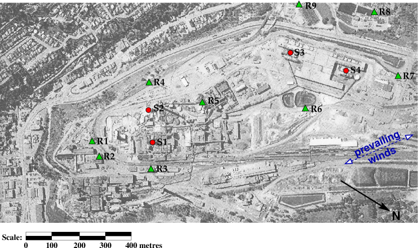
Figure 1: An aerial photo of the Trail site, showing the approximate locations of each of the sources (red circles, labeled by S$s$, $=1,2,3,4$) and receptors (green triangles, labeled R$r$, $r=1,2,\dots,9$). The size of the area depicted here is approximately $1600\times 800$ $\mathrm{m}$ and the directions of both the prevailing winds and compass north are indicated in the lower right corner.

Based on the above description, we now make a number of assumptions which are critical in the development of our dispersion model:

1. Each emission source is considered to be a point source, and all emission rates are constant in time, at least for any one-month period over which depositions are measured.

2. The wind velocity $\vec{u}(t)$ depends on time only and is uniform throughout the domain at any given instant. This is justifiable considering the relatively small dimensions of the site (1600 $\times$ 800 $\mathrm{m}$) and the short time intervals of interest.

3. Variations in topography are negligible so that the wind can be assumed horizontal. Although Trail is located in a river valley bordered by steep mountains, the domain of interest is far enough removed from the neighbouring mountain range that any topography or boundary effects can be ignored.

4. A ten-minute averaging period (or time step) is used in all calculations, which is consistent with the assumptions employed in deriving the Gaussian plume solution [23, 26] to limit errors in concentration.

5. Only dry deposition is considered since the dustfall measurements were all taken during months for which rainfall is relatively small.

6. The effects of plume rise are incorporated by using an “effective height” for each stack.

7. The atmospheric stability class is assumed to be class D (“neutral”, according to the Pasquill-Gifford classification scheme) for all monthly periods. There are insufficient meteorological data available to consider varying the stability class with time, and so our choice of neutral class is a compromise that takes into account predominant atmospheric conditions during the months of interest.

It is important to note that even though we focus our attention on an application to a specific industrial site, the mathematical model and associated numerical algorithms we develop are general and so can potentially be applied to a wide range of other atmospheric dispersion problems.

3 Derivation of the forward model

The release and transport of a single contaminant in the atmosphere can be described by the advection–diffusion equation

$$c_{t}+\vec{u}\cdot\nabla c=\nabla\cdot({\cal K}\nabla c)+S,$$ (1)

where

$c(\vec{x},t)=$	contaminant concentration [$\mathrm{kg\,m^{-3}}$],
$\vec{u}=$	convective wind velocity [$\mathrm{m\,s^{-1}}$],
${\cal K}(\vec{x})=$	$\operatorname{diag}(K_{x},K_{y},K_{z})$, the matrix of turbulent eddy diffusivities [$\mathrm{m^{2}\,s^{-1}}$],
$S(\vec{x},t)=$	emission source term [$\mathrm{kg\,m^{-3}\,s^{-1}}$].

We begin by considering a single elevated point source at location $(0,0,H)$ for which the source term takes the form

$$S(\vec{x},t)=Q\,\delta(x)\,\delta(y)\,\delta(z-H),$$ (2)

where $Q$ is a constant emission rate [$\mathrm{kg\,s^{-1}}$] and $\delta$ represents the Dirac delta function [$\mathrm{m^{-1}}$].  The coordinates $\vec{x}=(x,y,z)$ are chosen so that the $x$-axis is aligned parallel to the wind velocity. Although the wind velocity lies within the horizontal plane by our earlier assumption (2), there is nonetheless a small vertical velocity component $W_{\text{{set}}}$ that corresponds to gravitational settling. As a result, the velocity appearing in (1) takes the form $\vec{u}=(U(t),0,-W_{\text{{set}}})$, where $U(t)$ is the wind speed and the constant settling velocity is determined for spherical particles using Stokes’ law

$$W_{\text{{set}}}={\rho gd^{2}}/{(18\mu)},$$ (3)

where

$\rho=$	particle density [$\mathrm{kg\,m^{-3}}$],
$d=$	particle diameter [$\mathrm{m}$],
$\mu=$	air viscosity $=1.8\times 10^{-5}$ [$\mathrm{kg\,m^{-1}\,s^{-1}}$],
$g=$	gravitational acceleration $=9.8$ [$\mathrm{m\,s^{-2}}$].

Diffusive transport in the $x$-direction is typically much smaller than convective transport by the wind; hence, the diffusion term involving $K_{x}$ may be neglected, and $K_{y}(x)$ and $K_{z}(x)$ may be taken as functions of downwind distance only. As a result, Eq. (1) reduces to

$$\frac{\partial c}{\partial t}+U(t)\,\frac{\partial c}{\partial x}-W_{\text{{set}}}\,\frac{\partial c}{\partial z}=\\ \frac{\partial}{\partial y}\left(K_{y}\frac{\partial c}{\partial y}\right)+\frac{\partial}{\partial z}\left(K_{z}\frac{\partial c}{\partial z}\right)+S(\vec{x},t).$$ (4)

This equation could be modified to include vertical variations in both wind velocity and dispersion coefficients following [27, 28], although such effects will not be considered in this paper.

For the moment, we assume the domain is of infinite extent in the $x$ and $y$ directions, and the positive $z$ direction; consequently, we can apply the following Dirichlet boundary conditions at infinity:

$$c(x,\pm\infty,z) =0,$$ (5)

$$c(\pm\infty,y,z) =0,$$ (6)

$$c(x,y,\infty) =0.$$ (7)

The ground surface ($z=0$) is where deposition occurs, and so we impose the following mixed (Robin type) condition on particle flux

$$\left.\left(K_{z}\frac{\partial c}{\partial z}+W_{\text{{set}}}\,c\right)\right|_{z=0}=\left.W_{\text{{dep}}}\,c\right|_{z=0},$$ (8)

where $W_{\text{{dep}}}>0$ is the dry deposition velocity which is usually assumed constant and is determined from experiments.

3.1 Ermak’s solution

The Eqs. (4)–(8) have been well-studied and Ermak [6] derived the following analytical solution which is valid for $x>0$:

$$c(x,y,z)=\frac{Q}{2\pi U\sigma_{y}\sigma_{z}}\exp\left(-\frac{y^{2}}{2\sigma_{y}^{2}}\right)\\ \times\exp\left(-\frac{W_{\text{{set}}}\,(z-H)}{2K_{z}}-\frac{W_{\text{{set}}}^{2}\,\sigma_{z}^{2}}{8K_{z}^{2}}\right)\\ \times\left[\exp\left(-\frac{(z-H)^{2}}{2\sigma_{z}^{2}}\right)+\exp\left(-\frac{(z+H)^{2}}{2\sigma_{z}^{2}}\right)\right.\\ \left.-\;\sqrt{2\pi}\,\frac{W_{o}\,\sigma_{z}}{K_{z}}\;\exp\left(\frac{W_{o}(z+H)}{K_{z}}+\frac{W_{o}^{2}\,\sigma_{z}^{2}}{2K_{z}^{2}}\right)\right.\\ \times\left.\operatorname{erfc}\left(\frac{W_{o}\,\sigma_{z}}{\sqrt{2}\,K_{z}}+\frac{z+H}{\sqrt{2}\,\sigma_{z}}\right)\right],$$ (9)

where $W_{o}=W_{\text{{dep}}}-\frac{1}{2}W_{\text{{set}}}$. The quantities $\sigma_{y,z}(x)$ (having units of $\mathrm{m}$) represent standard deviations of concentration in the $y$ and $z$ directions and can be expressed in terms of the eddy diffusivities as

$$\sigma_{y,z}^{2}(x)=\frac{2}{U}\int_{0}^{x}K_{y,z}(x^{\prime})\,dx^{\prime}.$$

This integral simplifies to $K=\sigma^{2}U/2x$ when the eddy diffusivities are constant, although in practice the $\sigma$ values need to be taken as functions of the downwind distance $x$ in order to match observed plume concentrations.

Suppose that the height of a receptor above the ground is $z=h$; then the key quantity of interest is the contaminant deposition flux at $z=h$ which is given by the expression $W_{\text{{dep}}}c|_{z=h}$ from Eq. (8), with the height replaced by $z=h$. It is essential to observe that the deposition flux depends linearly on the emission rate $Q$ through Eq. (9), a fact that will be exploited to great advantage in this work.

3.2 Multiple sources and receptors

Instead of just a single point source, suppose instead that we have a set of $N_{s}$ sources, each with emission rate $Q_{s}$ [$\mathrm{kg\,s^{-1}}$] and location $\vec{\xi}_{s}$, for $s=1,2,\dots,N_{s}$. Likewise, there are $N_{r}$ receptors located at positions $\vec{\eta}_{r}$, each with total accumulated deposition $D_{r}$ [$\mathrm{kg}$], for $r=1,2,\dots,N_{r}$. On the Trail site depicted in Figure 1, there are $N_{s}=4$ sources and $N_{r}=9$ receptors that are of interest to this study. In the derivation that follows, we note that there are many similarities with Calder’s [7] general model framework for multiple-source emissions, except that he was unconcerned with deposition or any specific Gaussian plume approximation for the advection–diffusion equation.

In order to apply the solution from (9) for a uni-directional wind, a new set of transformed coordinates $\vec{\xi}_{s}$ must be defined for each source $s$ that translate the source location to the origin and then rotate coordinates so that the transformed $x$-axis is aligned parallel with the wind velocity. To this end, we define new coordinates $\vec{x}_{s}^{\,\prime}$ which are related to $\vec{x}$ via

$$\vec{x}_{s}^{\,\prime}={\cal R}_{-\theta}(\vec{x}-\vec{\xi}_{s}),$$ (10)

where $\theta$ corresponds to the angle the wind direction vector makes with the $x$-axis (measured counter-clockwise) and ${\cal R}_{-\theta}$ represents the matrix that rotates vectors through an angle $-\theta$ in the $x,y$-plane (see Figure 2). The resulting coordinates have an $x^{\prime}_{s}$–axis that is aligned with the wind direction.

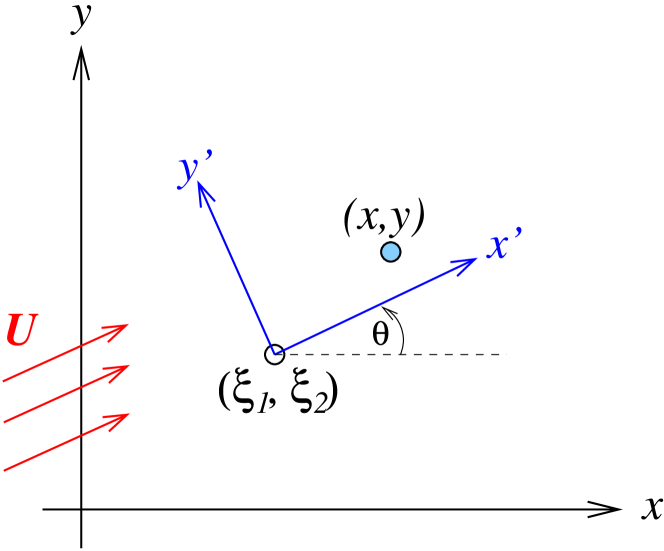
Figure 2: Relationship between the original coordinates $\vec{x}$ and transformed coordinates $\vec{x}^{\,\prime}$ for a given wind field having magnitude $U$ and direction angle $\theta$.

It is convenient to rewrite the concentration from (9) by factoring out the source emission rate and making the dependence on the source location and wind explicit, letting $c(\vec{x}_{s}^{\,\prime})=Q_{s}\,p(\vec{x};\vec{\xi_{s}},\theta,U)$. Consequently, the deposition flux may be written as

$$W_{\text{{dep}}}\,c|_{z=h}=W_{\text{{dep}}}\,Q_{s}\,p(\vec{x};\vec{\xi}_{s},\theta,U)|_{z=h},$$

and we may then calculate the total accumulation of contaminant in $\mathrm{kg}$ within a dustfall jar at location $\vec{x}$ over a time interval of length $\Delta t$ as

$$D(\vec{x}_{s}^{\,\prime})=\sum_{s=1}^{N_{s}}(W_{\text{{dep}}}\,Q_{s}A\Delta t)\,p(\vec{x};\vec{\xi}_{s},\theta,U),$$

where $A$ is the cross-sectional area $A$ of the jar opening. With a slight change in notation, we can write the total mass of a single contaminant deposited at receptor location $\vec{\eta}_{r}$ as

$$D_{r}=W_{\text{{dep}}}A\Delta t\sum_{s=1}^{N_{s}}Q_{s}\,p(\vec{\eta}_{r};\vec{\xi}_{s},\theta,U)|_{z=h_{r}}$$ (11)

which clearly indicates that the deposition is a linear combination of the emission rates $Q_{s}$.

3.3 Time-varying wind

Eqs. (11) are derived for a wind that is constant over the time interval of length $\Delta t$. In practice, the wind velocity varies with time and these variations have a significant impact on the plume dispersion and consequently also the deposition. The wind speed and direction, $U(t)$ and $\theta(t)$, are therefore both functions of time and so the coordinate transform (10) is also time-dependent. In order to make use of the Ermak solution, we divide time into $N_{t}$ equally-spaced intervals of length $\Delta t=T/N_{t}$, and assume that $U(t)$ and $\theta(t)$ can both be approximated by piecewise constant functions on each interval. The effects of time variation may then be incorporated by solving a sequence of Gaussian plume problems of the form (9) and the total mass deposited at receptor $r$ is calculated by summing the results over each time interval,

$$D_{r}^{tot}=W_{\text{{dep}}}A\Delta t\sum_{s=1}^{N_{s}}Q_{s}\sum_{n=1}^{N_{t}}p(\vec{\eta}_{r};\vec{\xi}_{s},\theta^{n},U^{n})|_{z=h_{r}},$$ (12)

where $p(\vec{x};\vec{\xi}_{s},\theta^{n},U^{n})$ represents the expression for the concentration, using averaged values of $U^{n}$ and $\theta^{n}$ corresponding to the $n^{th}$ time interval.

The Gaussian plume model assumes steady-state conditions, and so it is important to emphasize that we are making a major assumption when applying it to problems in which the wind velocity varies with time. As a result, the time step $\Delta t$ is a critical parameter: it must be chosen large enough that the plume can be considered sufficiently developed that it has reached a steady state, and yet not too large that the wind is seriously under-resolved. We choose a value of $\Delta t=10$ $\mathrm{min}$, motivated by a number of considerations:

• Since “typical” wind speeds lie between 1 and 5 $\mathrm{m\,s^{-1}}$, a given plume will be advected over a distance of 600 to 3000 $\mathrm{m}$, which is close to the 1000 $\mathrm{m}$ maximum separation between any individual source–receptor pair.

• Beychok [23] advocates an averaging interval of 10 minutes or less for the Gaussian plume model based on the observation that one-hour intervals can lead to over-prediction of the concentration by as much as a factor 2.5.

• Hanna et al. [26] note that Ermak’s solution is derived based on the assumption that all variables are averaged over time periods of approximately $10$ $\mathrm{min}$ in length.

Wind data is available down to a resolution of minutes, and so presents no limitation on the choice of $\Delta t$.

3.4 Parameter values and wind data

The physical parameters corresponding to the contaminant particles are summarized in Table 1. Because both zinc and strontium are deposited as sulphates, the parameters actually correspond to ZnSO₄ and SrSO₄. While zinc is the primary element of interest in this study, we will see in Section 4 that strontium is an important tracer element that plays a useful role in determining the solution to the inverse problem. The values for particle diameter and deposition velocity are consistent with data from [29, 30, 31], while the settling velocity is computed from Stokes’ law (3).

Table 1: Values of the physical parameters for the two contaminants of interest, where zinc and strontium actually appear in the form of sulphates – ZnSO₄ and SrSO₄. Note that the particle diameter and deposition velocity for Sr (marked $\ast$) have been set equal to those for Zn, in the absence of other more reliable estimates.

Parameter	Symbol	Units	Value for species $q=$
				Zn		Sr
Density	$\rho^{q}$	$\mathrm{kg\,m^{-3}}$		3540		3960
Molar mass	$M^{q}$	$\mathrm{kg\,mol^{-3}}$		0.161		0.184
Diameter	$d^{q}$	$\mathrm{\mu m}$		5		5∗
Deposition velocity	$W_{\text{{dep}}}^{q}$	$\mathrm{m\,s^{-1}}$		0.005		0.005∗
Settling velocity	$W_{\text{{set}}}^{q}$	$\mathrm{m\,s^{-1}}$		0.0027		0.0030
(from Eq. (3))

The heights of the four contaminant sources, corrected for plume rise, are $H_{s}=[15,35,15,15]$ while the nine receptors are located at heights $h_{r}=[0,10,10,1,15,2,3,12,12]$. The dustfall jars are glass containers in the shape of circular cylinders having a diameter of 0.162 $\mathrm{m}$, and so the area parameter used in the deposition calculation in Eq. (12) is $A=0.0206\;\mbox{$\mathrm{m^{2}}$}$.

The other key parameters appearing in the model are the standard deviations $\sigma_{y,z}$ which we assume take the form $\sigma(x)={ax}{(1+bx)^{-c}}$ customarily attributed to Briggs [32]. The constants appearing in this expression depend on the atmospheric stability class, and if we assume class D as discussed earlier then the values of the parameters are [33]:

for $$\sigma_{y} \quad a=0.08,\;\;b=0.0001,\;\;c=0.5,$$:

for $$\sigma_{z} \quad a=0.06,\;\;b=0.0015,\;\;c=0.5.$$:

The wind data for all simulations come from actual meteorological measurements taken on site and are specified as point measurements at 10-minute intervals. Figure 3 depicts the typical distributions of wind direction and velocity for a representative one-month period. The bimodal nature of the wind distribution in a direction aligned roughly parallel to the Columbia River valley is evident from the wind rose diagram.

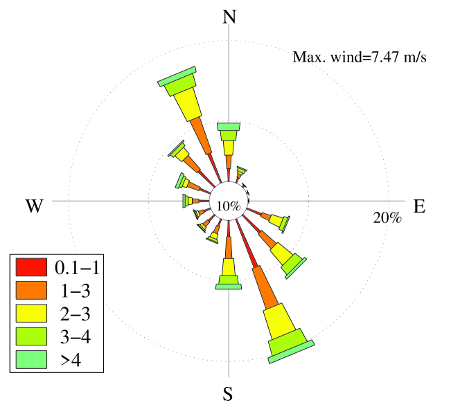
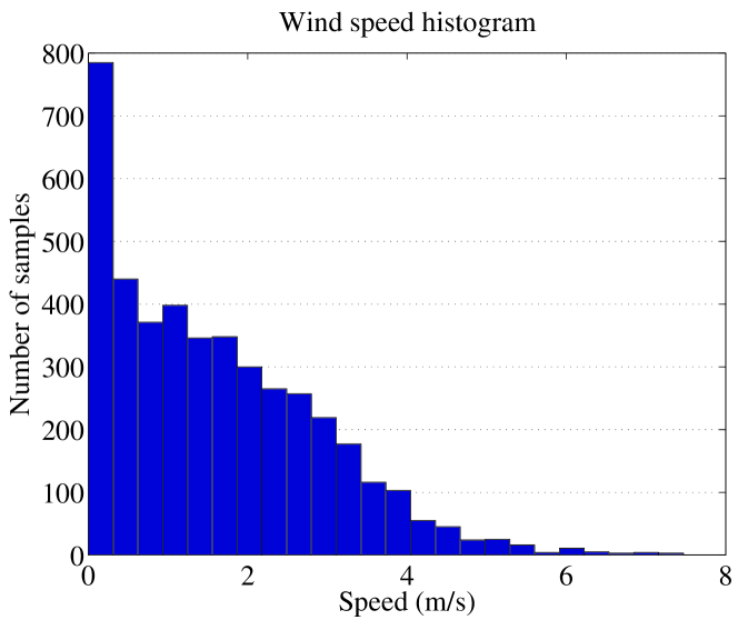
Figure 3: Measured wind data over the one-month period June 3–July 2, 2002. Top: Wind rose diagram, with the proportion of calm winds identified in the central circle. Bottom: Wind speed histogram.

A significant portion of wind measurements exhibit a zero velocity which cannot be used directly in Eq. (9). It is therefore usual to introduce a “cut-off” velocity $U_{\text{{min}}}$ such that whenever the wind satisfies $U\leqslant U_{\text{{min}}}$, no contribution is made to the deposition during that time interval. We employ a cut-off of $U_{\text{{min}}}=0.1$ which limits the number of neglected time intervals to 10% of the total.

3.5 Sample forward computation

Using the parameter values given in the previous section, we next calculate a typical distribution of the zinc ground-level concentrations using the time-varying plume solution (12). The emission rates for the four sources were taken to be $\vec{Q}=[35,80,5,5]\times 10^{3}$ $\mathrm{kg\,yr^{-1}}$, and measured wind data at 10 minute intervals was used for the month of June 2002. The mass of zinc deposited at each receptor was then computed to 3 significant digits as

$$\begin{split}\vec{D}=&\left[\;17.4,\,31.0,\,15.7,\,1.63,\,21.7,\right.\\ &\left.\;\;6.33,\,2.54,\,5.02,\,7.74\;\right]\times 10^{-6}\;\mbox{$\mathrm{kg}$}.\end{split}$$ (13)

We also computed ground-level zinc concentrations on a 100 $\times$ 100 grid of points covering the entire Trail site, and the results are displayed as a contour plot in Figure 4. The concentration clearly peaks at locations that lie close to sources S1 and S2 and aligned with the prevailing wind direction. This is to be expected since S1 and S2 have by far the largest emission rates among the four sources.

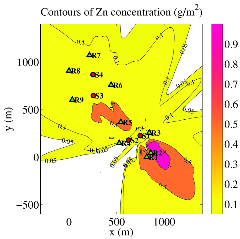
Figure 4: Forward simulation of the monthly cumulative deposition of zinc (in $\mathrm{g\,m^{-2}}$) at each point in the domain for source emission rates $\vec{Q}=[35,80,5,5]\times 10^{3}$ $\mathrm{kg\,yr^{-1}}$. The wind data used to generate this plot corresponds to June 2002, for which the dominant wind direction is towards the southeast. Note that compass north is directed vertically in this plot, which is rotated relative to the aerial photo in Fig. 1.

4 Inverse problem

We now consider the inverse problem for which values of the zinc deposition $D_{r}$ are specified at each receptor $r=1,2,\dots,N_{r}$, and the unknowns are the source emission rates $Q_{s}$ for $s=1,2,\dots,N_{s}$. It is convenient to rewrite Eqs. (12) in the more compact form

$$\vec{D}=\mathbb{P}\,\vec{Q}$$ (14)

where $\vec{D}$ and $\vec{Q}$ are vectors containing the depositions and emission rates respectively, and $\mathbb{P}$ is an $N_{r}\times N_{s}$ matrix whose $r,s$ entry is given by

$$\mathsf{P}_{rs}=W_{\text{{dep}}}A\Delta t\,\sum_{n=1}^{N_{t}}p(\vec{\eta}_{r};\vec{\xi}_{s},\theta^{n},U^{n})|_{z=h_{r}}.$$ (15)

Since there will typically be more receptor measurements than sources ($N_{r}>N_{s}$), this is clearly an overdetermined system of equations for $\vec{Q}$; hence, there is not a unique solution and we can hope at best to obtain an approximation of $\vec{Q}$.

We employ a linear least squares method to determine a solution of Eq. (14), and in all of our computations we employ the lsqlin solver in MATLAB. A typical simulation requires only about 20 $\mathrm{s}$ of CPU time on a MacBook Pro with a 2.5 GHz Intel dual-core processor, and so our method is very efficient and well-suited to performing parametric studies. MacKay et al. [15] used a similar least squares method to estimate parameters such as surface mass transfer rate and Péclet number rather than emission rates.

As a consistency check on our inverse algorithm, we consider emissions of a single contaminant (zinc) under the influence of wind data during the month of June 2002. Deposition values are taken equal to the outputs from the forward computation in Eq. (13), with all other parameters chosen the same. As expected, the emission rates calculated with the inverse algorithm are identical to within round-off error.

4.1 Multiple contaminants and linear constraints

As mentioned earlier, dustfall measurements are made of several contaminants, not just zinc. The contents of each receptor underwent a trace analysis that measures the mass of a number of trace elements, of which we are interested in zinc, strontium and sulphur (in the form of SO₄). Although zinc is the contaminant of primary interest in this study, the sulphur and strontium arise from the same chemical processes that produce zinc, and consequently we have included them in the inversion procedure with the hope that they will increase the accuracy of the zinc estimate. Because zinc and strontium are deposited as sulphates, the emission rate of sulphur cannot be included as an independent variable and so we need to estimate emission rates for only zinc and strontium.

By modifying our previous notation slightly, we can identify contaminant species with a superscript $q$ in the emission rates $\vec{Q}_{s}^{q}$ (where $q=$ Zn or Sr) and depositions $\vec{D}_{r}^{q}$ ($q=$ Zn, Sr or SO₄). Our task is then to solve the following three linear systems

$$\begin{split}\vec{D}^{\text{Zn}}&=\mathbb{P}^{\text{Zn}}\,\vec{Q}^{\text{Zn}},\\ \vec{D}^{\text{Sr}}&=\mathbb{P}^{\text{Sr}}\,\vec{Q}^{\text{Sr}},\\ \vec{D}^{\text{SO${}_{4}$}}&=\frac{M^{\text{SO${}_{4}$}}}{M^{\text{Zn}}}\mathbb{P}^{\text{Zn}}\vec{Q}^{\text{Zn}}+\frac{M^{\text{SO${}_{4}$}}}{M^{\text{Sr}}}\mathbb{P}^{\text{Sr}}\vec{Q}^{\text{Sr}}\end{split}$$ (16)

where the matrices $\mathbb{P}^{q}$ are given in (15) and depend on the contaminant $q$ through the deposition velocity $W_{\text{{dep}}}^{q}$ and settling velocity $W_{\text{{set}}}^{q}=g\,\rho^{q}\,(d^{q})^{2}/18\mu$. Since the scenario we are studying has $N_{s}=4$ sources and $N_{r}=9$ receptors, Eqs. (16) represent an overdetermined system of 27 equations in 8 unknowns. Once $\vec{Q}^{\text{Zn}}$ and $\vec{Q}^{\text{Sr}}$ are known, the emission rate for sulphate can be obtained from

$$\vec{Q}^{\text{SO${}_{4}$}}=\frac{M^{\text{SO${}_{4}$}}}{M^{\text{Zn}}}\vec{Q}^{\text{Zn}}+\frac{M^{\text{SO${}_{4}$}}}{M^{\text{Sr}}}\vec{Q}^{\text{Sr}}.$$ (17)

In addition to the atmospheric transport processes embodied by the above equations, the chemical processes generating the contaminants introduce a number of further constraints on the emission rates. To be more specific, we note that source S1 corresponds to a collection of zinc purification stacks, S2 is a sulphide leach plant cooling tower, and S3 and S4 are identical electrolytic cooling stacks. As a result, we can make the following assumptions:

• Sources 3 and 4 are identical:

  $$Q_{3}^{q}-Q_{4}^{q}=0,\quad\text{for $q=$ \text{Zn}, \text{Sr}}.$$ (18)

• The mass ratio of zinc to strontium in sources 3 and 4 is approximately 6000 to 1:

  $$Q_{s}^{\text{Zn}}-6000Q_{s}^{\text{Sr}}=0\quad\text{for $s=3,4$}.$$ (19)

• No strontium is emitted from sources 1 and 2:

  $$Q_{1}^{\text{Sr}}=Q_{2}^{\text{Sr}}=0.$$ (20)

• All emission rates must be non-negative:

  $$Q_{s}^{\text{Zn}},\;\;Q_{s}^{\text{Sr}}\geqslant 0\quad\text{for $s=1,2,3,4$}.$$ (21)

When taken together, Eqs. (18)–(21) represent 6 equality and 8 inequality constraints that supplement the overdetermined system (16). We can therefore continue to make use of the MATLAB linear least squares solver lsqlin which conveniently permits the inclusion of both equality and inequality constraints.

5 Numerical simulations

5.1 Base case

We begin by focusing on a number of inverse calculations using a single month of wind and deposition data corresponding to June 2002 – we refer to this simulation as the “base case.” The receptor measurements used as inputs are displayed in Fig. 5, while the wind data is the same as that shown earlier in Fig. 3.

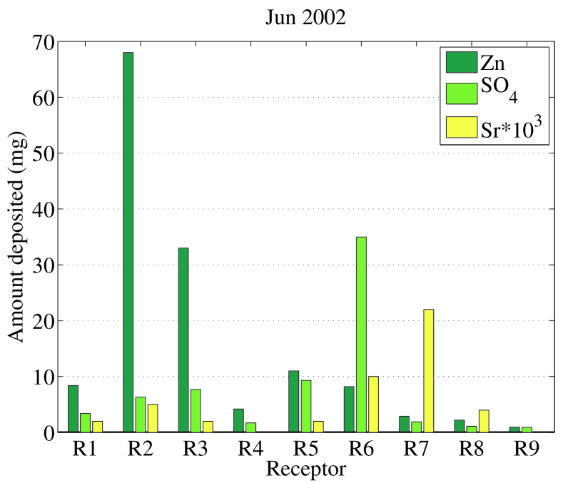
Figure 5: Experimental measurements of the mass of contaminants accumulated within each receptor during the month of June 2002. The zinc and sulphate figures are shown in units of $\mathrm{mg}$, while strontium is scaled by $10^{3}$ so that it is visible on the same axes.

The estimated source emission rates are displayed in Fig. 6 in units of tonnes per year. We are primarily interested in zinc emissions, which come to a total of $92.44\;\mbox{$\mathrm{T\,yr^{-1}}$}$ for all four sources. This total should be compared with the figure of 116.48 $\mathrm{T\,yr^{-1}}$ reported by Teck-Cominco in the National Pollutant Release Inventory for the year 2002 [25]. The fact that these two figures are so close gives us some confidence that our inverse approach for estimating emissions is a reasonable one. We have not attempted a comparison between the other two contaminants because strontium emissions are not reported to NPRI, and our model does not account for all sources of atmospheric sulphate emissions on the Trail site.

Figure 6: Estimated emissions rates for the “base case” corresponding to June 2002 (the strontium value is scaled by $10^{4}$).

5.2 Parameter sensitivities

In this section, we investigate the sensitivity of our inverse solution to changes in several key parameters, namely receptor height ($h_{r}$), source height ($H_{s}$) and deposition velocity ($W_{\text{{dep}}}^{q}$). These parameters are singled out because they are all subject to significant variations for the following reasons:

• There is a great deal of freedom in the placement of individual receptors, which for example can be located at ground level or else on the top of buildings or other structure.

• The height of each source must be adjusted to take into account the effect of plume rise, which can be estimated using empirical formulas but there remains a significant degree of uncertainty in these plume rise estimates.

• Particle deposition velocities are known to depend strongly on atmospheric conditions and on whether deposition happens under dry or wet conditions.

We perform a series of simulations, modifying each parameter by $\pm 10$% and $\pm 20$% from the base case value. The resulting emission estimates are compared in Figs. 7, 8 and 9 for parameters $h_{r}$, $H_{s}$ and $W_{\text{{dep}}}^{q}$ respectively. Only zinc emission rates are depicted here since similar levels of sensitivity are experienced for the other contaminants.

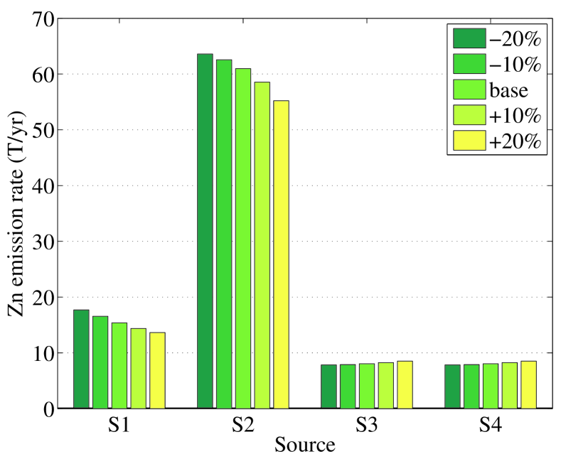
Figure 7: Effect of changes in receptor height $h_{r}$ on Zn emission rates.

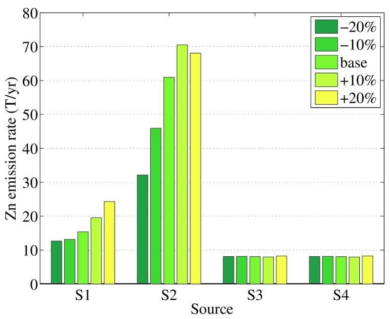
Figure 8: Effect of changes in source height $H_{s}$ on Zn emission rates.

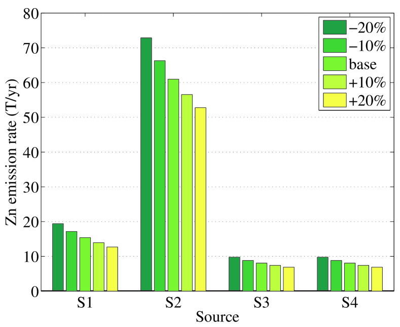
Figure 9: Effect of changes in deposition velocities $W_{\text{{dep}}}^{q}$ on Zn emission rates.

From these results, we conclude that the solution is most sensitive to source height, where relative changes on the order of 40–50% are seen. Much less variation is seen in response to changes in $H$ and $W_{\text{{dep}}}$. These sensitivities are consistent with Miller and Hively [34], who reviewed a wide range of Gaussian plume type models and found that for elevated sources, ground-level concentrations are typically estimated to within a factor of 0.65 to 1.35 of the actual values.

5.3 Noise in deposition measurements

Even though we expect that the emission rates should remain approximately constant over time (at least during a given year) there is nonetheless a significant spread in deposition measurements from month to month. There are a number of possible explanations for this variation, including measurement errors, wet deposition during rainy periods (where “scrubbing” can significantly reduce the amount deposited) or contamination from secondary sources not accounted for in the model. Indeed, Goodarzi et al. [24] performed an experimental study of emissions at the Teck Cominco’s Trail operation and determined that secondary sources on the site (such as ore concentrate and slag storage piles) experience resuspension of particles which may interfere with deposition measurements.

In any case, it is important to understand the effect that possible errors in particulate measurements may have on emission estimates. To this end, we take each deposition measurement and scale it by a normally distributed random number chosen from the interval $[1-\alpha,1+\alpha]$ for values of $\alpha=0.1$, 0.2 and 0.3. The results are summarized in Fig. 10, from which it is clear that even for the largest noise ratio $\alpha=0.3$, the corresponding errors in the computed emission rates are relatively small. One possible explanation for this limited sensitivity to noise is that positive and negative contributions to errors in the input data may cancel each other out on average.

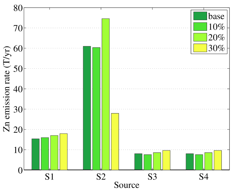
Figure 10: Effect of random noise in deposition measurements on Zn emission rates.

5.4 A note on ill-conditioning

Our approach does not suffer from the extreme levels of sensitivity observed by others in inverse computations based on Gaussian plume type solutions (for example, [34], [35] and [36]). We can explain this apparent discrepancy by noting that our simulations are performed over relatively short time periods as well as being restricted to ground level and to areas very close to the emission source. In contrast, Enting and Newsam’s study of the inverse emissions problem indicated that computed concentrations at distances further than 10 $\mathrm{km}$ downwind from a source are highly sensitive when high-altitude pollutant measurements are used. Although these and other studies of atmospheric dispersion focus on long-range transport (over 10’s or even 100’s of $\mathrm{km}$) our approach benefits from the fact that we consider transport over much shorter spatial scales.

5.5 Deposition over several months

Deposition measurements are available for a total of six monthly periods: June, October and November in 2001; and May, June and July in 2002. All of these measurements correspond to periods during which the Trail smelter was in continuous operation without being shut down; therefore, one would expect the depositions to be fairly consistent from month to month. The measured values for zinc are summarized in Fig. 11, from which we observe that there are significant variations at each receptor location over time, although the trend is fairly consistent between one receptor and another. Furthermore, the largest accumulations are consistently measured in receptors located closest to the primary sources S1 and S2, as expected. Similar trends are observed in the strontium and sulphate data and so they are not depicted.

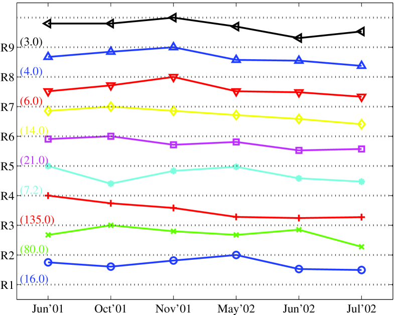
Figure 11: Simulated Zn deposition rates for every monthly period under consideration. For each receptor, the axis limits are drawn as horizontal dotted lines and are scaled so that the lower limit is zero and the upper limit represents the maximum deposition rate (given by the number in parentheses to the left of each curve in $\mathrm{T\,yr^{-1}}$).

Keeping in mind our earlier discussion in Section 5.3 of the solution sensitivity to the error in deposition data, we next apply our inverse algorithm for each one-month periods individually. The resulting monthly emission rate estimates for zinc are given in the bar plot in Fig. 12.  There is considerable variation between the results for individual months, which is not surprising considering the variations in the input data. Furthermore, two of the S2 estimates (corresponding to June 2001 and July 2002) are identically zero, indicating that the least squares algorithm has forced the S2 value up against the boundary of the inequality constraint $Q_{3}^{\text{Zn}}\geqslant 0$. These two results are clearly questionable because S2 is by far the largest source of zinc on the site.

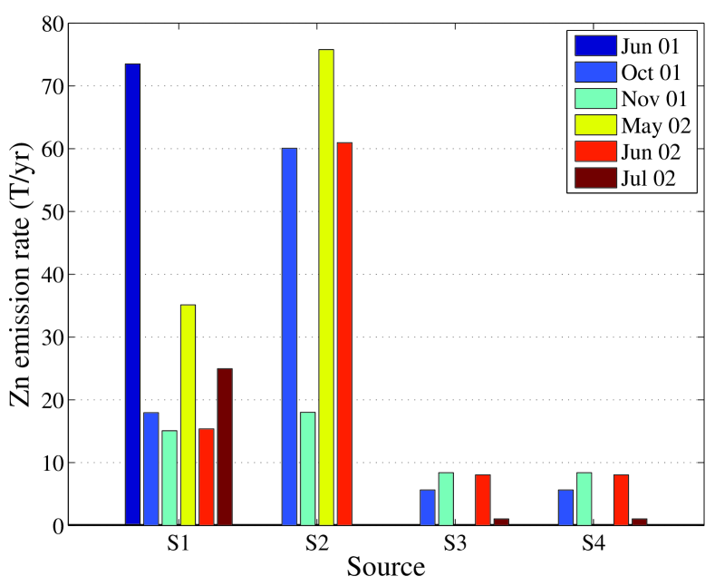
Figure 12: Computed Zn emission rates for each monthly period.

With an aim to explaining this discrepancy, we take a closer look at the zinc deposition data in Fig. 11 and observe that the R3 deposition measurements are unusually high in relation to other nearby receptors (in particular, see the peak value of 135 $\mathrm{mg}$ measured in June 2001). Instead, one would expect that the values at R3 and R4 are much closer to each other since their location relative to the primary sources S1 and S2 is so similar. Furthermore, it seems reasonable that the maximum deposition should occur at a point lying to the southeast or northwest of sources S1 and S2, rather than at R3 which is perpendicular to the direction of the prevailing winds. We conclude therefore that the large deposition at R3 is most likely attributable to measurement errors or some other anomaly, and hence R3 should be excluded from the calculations.

Upon repeating the previous set of simulations with R3 excluded, we obtain the results shown in Fig. 13. All S1 and S2 emission estimates are now nonzero and the anomalously high S1 estimate for June 2002 is reduced to be in more line with the other values. Although there remain significant variations between a few of the monthly estimates (namely November 2001 and July 2002), these results are much more reasonable.

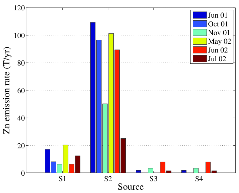
Figure 13: Computed Zn emission rates for each monthly period, leaving out receptor R3 (compare to Fig. 12).

Since the primary quantity of interest in this study is the total emissions from all sources, another way of viewing these results is via the total emissions from all four sources for each monthly period, as shown in Fig. 14.

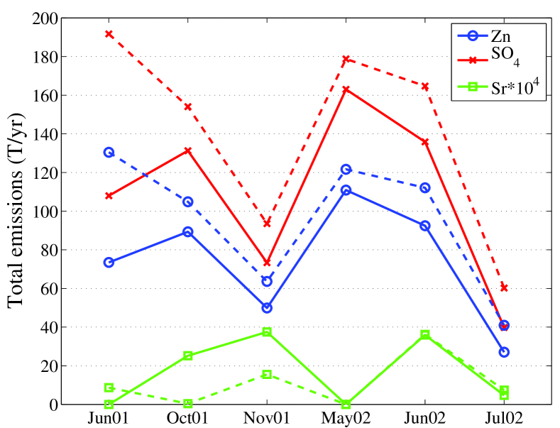
Figure 14: Total emissions for each contaminant. The solid lines correspond to simulations with R3 included in the inverse calculation, while the dashed lines are without R3.

If we assume that emissions are constant throughout the year, then we may also use all months of deposition data from a given year to estimate a single “aggregate” emission rate. The aggregate estimates based on the 2001 and 2002 data are shown in Table 2 along with the total emission rates for the individual months. One advantage of using the aggregate calculation is that it serves to average out some of the variation between the individual monthly results. The aggregate figures can then be compared to the values from the NPRI database of 100.33 $\mathrm{T\,yr^{-1}}$ in 2001 and 116.48 $\mathrm{T\,yr^{-1}}$ in 2002. For both years, the aggregate estimates are within 10-20% of the reported values, and an increasing trend from 2001 to 2002 is also captured.

Table 2: Summary of total zinc emissions for each month of interest, the corresponding aggregate totals for each year, and the emissions reported to NPRI. Receptor R3 is omitted.

	Zn Emission rates ($\mathrm{T\,yr^{-1}}$)
	2001	2002
Monthly estimates	130.5	121.7
	104.9	112.1
	63.64	40.97
Aggregate estimates	95.77	104.5
Reported to NPRI[25]	100.33	116.48

6 Conclusions

We have derived a linear least squares approach for estimating contaminant emissions from several point sources given time-varying wind data and monthly-averaged deposition measurements. The model is based on Ermak’s Gaussian plume type solution to the advection-diffusion equations [6] which incorporates particle settling and surface deposition. The novelty of our approach stems from its focus on short range emissions (within 1000 $\mathrm{m}$ of the source), incorporating additional equality and inequality constraints on contaminant sources, and its ability to handle time-varying wind data.

The algorithm is used to estimate emissions of several contaminants from a smelting operation in Trail, British Columbia using dustfall measurements taken over several one-month periods during 2001–2002. We demonstrate that the algorithm is efficient and robust to changes in several key parameter values in comparison to other approaches published in the literature. While there is significant variation from month-to-month and between the individual sources, the average annual estimate of the emission rate is within 10–20% of the values reported to Environment Canada for the years in question.

There remain a number of aspects of the model which require further study and refinement, for example by using more careful estimates of the contribution of plume rise to source heights, incorporating the effects of wet deposition during rainy periods, and allowing further variation in atmospheric conditions through the Pasquill-Gifford stability classification. We would also like to apply our insight into contaminant plume dynamics to guide the design of future studies of the Trail site; in particular, by relocating a receptor such as R3 to a more advantageous position (e.g., within the areas of peak concentration southeast or northwest of sources S1 and S2). Finally, we will perform a direct finite volume discretization of the 3D advection-diffusion equation, for which reliable estimates for the turbulent eddy diffusivities are essential. Comparisons of these simulations with the results of our inverse Gaussian plume algorithm will appear in a companion publication [37].

References

- [1] D. B. Turner, Atmospheric dispersion modeling: A critical review, Journal of the Air Pollution Control Association 29 (5) (1979) 502–519.
- [2] G. S. Settles, Fluid mechanics and homeland security, Annual Review of Fluid Mechanics 38 (2006) 87–110.
- [3] L. F. Richardson, Some measurements of atmospheric turbulence, Philosophical Transactions of the Royal Society of London A 221 (1921) (1920) 1–28.
- [4] G. I. Taylor, Diffusion by continuous movements, Proceedings of the London Mathematical Society (1922) 196–212.
- [5] O. G. Sutton, A theory of eddy diffusion in the atmosphere, Proceedings of the Royal Society of London, Series A 135 (826) (1932) 143–165.
- [6] D. L. Ermak, An analytical model for air pollutant transport and deposition from a point source, Atmospheric Environment 11 (3) (1977) 231–237.
- [7] K. L. Calder, Multiple-source plume models of urban air pollution – Their general structure, Atmospheric Environment 11 (1977) 403–414.
- [8] J. B. Liley, Analytic solution of a one-dimensional equation for aerosol and gas dispersion in the stratosphere, Journal of the Atmospheric Sciences 52 (18) (1995) 3283–3288.
- [9] J.-S. Lin, L. M. Hildemann, A generalized mathematical scheme to analytically solve the atmospheric diffusion equation with dry deposition, Atmospheric Environment 31 (1) (1997) 59–71.
- [10] S. A. Condie, M. Bormans, The influence of density stratification on particle settling, dispersion and population growth, Journal of Theoretical Biology 187 (1997) 65–75.
- [11] A. El Badia, T. Ha-Duong, A. Hamdi, Identification of a point source in a linear advection-dispersion-reaction equation: application to a pollution source problem, Inverse Problems 21 (2005) 1121–1136.
- [12] C. Kennedy, H. Ericsson, P. L. R. Wong, Gaussian plume modeling of contaminant transport, Stochastic and Environmental Risk Assessment 20 (2005) 119–125.
- [13] H.-J. Jeong, E.-H. Kim, K.-S. Suh, W.-T. Hwang, M.-H. Han, H.-K. Lee, Determination of the source rate released into the environment from a nuclear power plant, Radiation Protection Dosimetry 113 (3) (2005) 308–313.
- [14] W. R. Hogan, G. F. Cooper, M. M. Wagner, G. L. Wallstrom, An inverted Gaussian plume model for estimating the location and amount of release of airborne agents from downwind atmospheric concentrations, RODS technical report, Realtime Outbreak and Disease Surveillance Laboratory, University of Pittsburgh, Pittsburgh, PA (2005).
- [15] C. MacKay, S. McKee, A. J. Mulholland, Diffusion and convection of gaseous and fine particulate from a chimney, IMA Journal of Applied Mathematics 71 (2006) 670–691.
- [16] M. Mulholland, J. H. Seinfeld, Inverse air pollution modelling of urban-scale carbon monoxide emissions, Atmospheric Environment 29 (4) (1995) 497–516.
- [17] P. Seibert, A. Frank, Source-receptor matrix calculation with a Lagrangian particle dispersion model in backward mode, Atmospheric Chemistry and Physics 4 (2004) 51–63.
- [18] I. G. Enting, Inverse Problems in Atmospheric Constituent Transport, Cambridge Atmospheric and Space Science Series, Cambridge University Press, 2002.
- [19] A. Goyal, M. J. Small, K. von Stackelberg, D. Burmistrov, N. Jones, Estimation of fugitive lead emission rates from secondary lead facilities using hierarchical Bayesian models, Environmental Science and Technology 39 (13) (2005) 4929–4937.
- [20] A. C. Bagtzoglou, S. A. Baun, Near real-time atmospheric contamination source identification by an optimization-based inverse method, Inverse Problems in Science and Engineering 13 (3) (2005) 241–259.
- [21] M. Brown, Deduction of emissions of source gases using an objective inversion algorithm and a chemical transport model, Journal of Geophysical Research 98 (D7) (1993) 12639–12660.
- [22] S. Houweling, T. Kaminski, F. J. Dentener, J. Lelieveld, M. Heimann, Inverse modeling of methane sources and sinks using the adjoint of a global tranport model, Journal of Geophysical Research 104 (D21) (1999) 26137–26160.
- [23] M. R. Beychok, Error propagation in air dispersion modeling, ChemAlliance.org, http://www.chemalliance.org/Articles/Industry/Ind990816.asp (16 August 1999).
- [24] F. Goodarzi, H. Sanei, M. Labonté, W. F. Duncan, Sources of lead and zinc associated with metal smelting activities in the Trail area, British Columbia, Canada, Journal of Environmental Monitoring 4 (2002) 400–407.
- [25] National pollutant release inventory, Environment Canada, URL: http://www.ec.gc.ca/pdb, accessed on April 27, 2009 (Trail, British Columbia, NPRI ID #3802).
- [26] S. R. Hanna, G. A. Briggs, R. P. Hosker Jr., Handbook on atmospheric diffusion, Tech. Rep. DOE/TIC-11223, Technical Information Center, U.S. Department of Energy (1982).
- [27] C. V. Chrysikopoulos, L. M. Hildemann, P. V. Roberts, A three-dimensional steady-state atmospheric dispersion-deposition model for emissions from a ground-level area source, Atmospheric Environment 26A (5) (1992) 747–757.
- [28] W. Koch, A solution of the two-dimensional atmospheric diffusion equation with height-dependent diffusion coefficient including ground level absorption, Atmospheric Environment 23 (8) (1989) 1729–1732.
- [29] D. F. Gatz, Pollutant aerosol deposition into southern Lake Michigan, Water, Air and Soil Pollution 5 (1975) 239–251.
- [30] T. A. McMahon, P. J. Denison, Empirical atmospheric deposition parameters – A review, Atmospheric Environment 13 (1979) 571–585.
- [31] J. M. Pacyna, A. Bartonova, P. Cornille, W. Maenhaut, Modelling of long-range transport of trace elements. A case study, Atmospheric Environment 23 (1) (1989) 107–114.
- [32] G. A. Briggs, Diffusion estimation for small emissions, Atmospheric Turbulence and Diffusion Laboratory Contribution, File No. 79, National Oceanic and Atmospheric Administration, Oak Ridge, TN (1973).
- [33] M. D. Carrascal, M. Puigcerver, P. Puig, Sensitivity of Gaussian plume model to dispersion specifications, Theoretical and Applied Climatology 48 (1993) 147–157.
- [34] C. W. Miller, L. M. Hively, A review of validation studies for the Gaussian plume atmospheric dispersion model, Nuclear Safety 28 (4) (1987) 522–531.
- [35] I. G. Enting, G. N. Newsam, Atmospheric constitutent inversion problems: Implications for baseline monitoring, Journal of Atmospheric Chemistry 11 (1990) 69–87.
- [36] I. G. Enting, G. N. Newsam, Inverse problems in atmospheric constituent studies: II. Sources in the free atmosphere, Inverse Problems 6 (1990) 349–362.
- [37] E. Lebed, J. M. Stockie, A high-resolution finite volume approach for the transport of particulate emissions in the atmosphere, In preparation.