Phase diagram for asymmetric nuclear matter in the multifragmentation model

Abstract

We assume that, in equilibrium, nuclear matter at reduced density and moderate finite temperature, breaks up into many fragments. A strong support to this assumption is provided by data accumulated from intermediate energy heavy ion collisions. The break-up of hot and expanded nuclear matter according to rules of equilibrium statistical mechanics is the multifragmentation model. The model gives a first-order phase transition. This is studied in detail here. Phase-equilibrium lines for different degrees of asymmetry are computed.

I Introduction

Nuclear matter is a hypothetical very large system of nucleons where the Coulomb effects of protons are switched off. Such a system is expected to have features of liquid-gas phase transition. We consider here the equation of state of symmetric and asymmetric nuclear matter at temperature between 4 and 10 MeV and at less than half of normal nuclear density. We assume that at equilibrium at finite temperature (three to tens of MeV) and low average density, nuclear matter breaks up into fragments, each with normal nuclear density. Strong support to this assumption comes from data on heavy ion collisions but it is also supported by theoretical modelling. For example it can be easily shown (see section IV in Bhatta ), using Skyrme type interaction, that the free energy of uniformly stretched nuclear matter is very significantly lowered if the matter is allowed to split into many fragments, each with normal nuclear density. This is the multifragmentation model. We use this model to study thermodynamic properties of nuclear matter, particularly phase-equilibrium lines (the lines of co-existence of liquid and gas phases) in the $p-T$ plane for both symmetric and asymmetric matter.

This is an extension of the model described in our earlier work Chaudhuri1 where only one kind of particles was considered. This one kind of particles however formed clusters whose properties were patterned after actual finite nuclei. While we hope that the present article is self-contained we will refer to this earlier work for elucidation of some points. There is a large number of publications on equation of state and phase transitions in nuclear matter. Ref. De1 comes closest to the spirit of this paper. While there are quite a few common features with this work there are also some differences and we highlight some other aspects. Phase transition in nuclear matter using mean-field theory was studied over many years and we can not attempt an adequate bibliography here. We mention two papers which critically looked at asymmetric nuclear matter and received a great deal of attention in very recent times Muller ; Ducoin . Both of these use mean-field theories and overcome the difficulty of instability through Maxwell construction. The multifragmentation approach is very different. It is more directly related to actual observables but in its present form it can only be trusted in a low density regime. But there is no need for Maxwell construction.

II The Formulae

We briefly review the grand canonical model for multifragmentation Dasgupta1 . Let the numbers of neutrons and protons in the dissociating system be $N_{0}$ and $Z_{0}$ respectively. At finite temperature and in subnormal densities, these will break up into all possible composites each with some neutrons($N$) and protons ($Z$)(mass number $A=N+Z$). We always use the subscripted $N_{0},Z_{0}$ to refer to the very large system whose thermodynamic properties are being investigated whereas $N,Z$ refer to composites which can be small or large. The properties of the composites are determined by the basic two-body interactions These properties are utilized in the model but interactions between composites are neglected (except through excluded volume effect; see discussion later) by appealing to the short range nature of nuclear forces. This limits the validity of the model to low densities. Here we will restrict our investigation to densities $\rho/\rho_{0}$ to 0.5 or less where $\rho_{0}$ is the normal nuclear density. This is the customary practice Das1 .

If the neutron chemical potential is $\mu_{n}$ and the proton chemical potential is $\mu_{p}$, then statistical equilibrium implies that the chemical potential of a composite with $N$ neutrons and $Z$ protons is $\mu_{n}N+\mu_{p}Z$. The following are the relevant equations for us. The average number of composites with $N$ neutrons and $Z$ is ($\beta=1/T$)

$$\langle n_{N,Z}\rangle=e^{\beta\mu_{n}N+\beta\mu_{p}Z}\omega_{N,Z}$$ (1)

Here $\omega_{N,Z}$ is a one body partition function for the composite $(N,Z)$. It is a product of two factors; one arising from the translational motion of the composite and another from the intrinsic partition function of the composite:

$$\omega_{N,Z}=\frac{V_{f}}{h^{3}}(2\pi mT)^{3/2}A^{3/2}\times z_{N,Z}(int)$$ (2)

Here $V_{f}$ is the volume available for translational motion; $V_{f}$ will be less than $V$, the volume to which the system has expanded at break up (excluded volume correction). We use $V_{f}=V-V_{0}$ , where $V_{0}$ is the normal volume of nucleus with $Z_{0}$ protons and $N_{0}$ neutrons. The quantity $z_{N,Z}(int)$ depends upon the intrinsic properties of the composites and contains all the nuclear physics.

We list now the properties of the composites used in this work. The proton and the neutron are fundamental building blocks thus $z_{1,0}(int)=z_{0,1}(int)=2$ where 2 takes care of the spin degeneracy. For deuteron, triton, ³He and ⁴He we use $z_{i,j}(int)=(2s_{i,j}+1)\exp(-\beta e_{i,j}(gr))$ where $e_{i,j}(gr)$ is the ground state energy of the composite and $(2s_{i,j}+1)$ is the experimental spin degeneracy of the ground state. Because we are modeling a system where protons do not carry any charges the ground state energy of ³He is taken to be that of the triton and the Coulomb energy is subtracted from the experimental energy of the alpha particle. These modifications make insignificant changes. Excited states for these very low mass nuclei are not included. For mass number $a=5$ and greater we use the liquid-drop formula. This reads

$$z_{i,j}(int)=\exp[-\frac{F_{i,j}}{T}]$$ (3)

Here $F_{i,j}$ is the internal free energy of species $(i,j)$:

$$F_{i,j}=-W_{0}a+\sigma(T)a^{2/3}+s\frac{(i-j)^{2}}{a}-\frac{T^{2}a}{\epsilon_{0}}.$$ (4)

The expression includes the volume energy, the temperature dependent surface energy and the symmetry energy. The values of the paprameters are taken from Bondorf1 . The term $\frac{T^{2}a}{\epsilon_{0}}$ represents contribution from excited states since the composites are at a non-zero temperature. For nuclei with $A$=5 we include $Z$=2 and 3 and for $A$=6 we include $Z$=2,3 and 4. For higher masses we compute the drip lines using the liquid-drop formula above and include all isotopes within these boundaries.

There are two equations which determine $\mu_{n}$ and $\mu_{p}$.

$$N_{0}=\sum Ne^{\beta\mu_{n}N+\beta\mu_{p}Z}\omega_{N,Z}$$ (5)

$$Z_{0}=\sum Ze^{\beta\mu_{n}N+\beta\mu_{p}Z}\omega_{N,Z}$$ (6)

We want to point out the following feature of the grand canonical model. In all $\omega_{N,Z}$’s in the sum in the above two equations, there is one common value for $V_{f}$ (see eq.(2)). We really solve for $N_{0}/V_{f}$ and $Z_{0}/V_{f}$. The values of $\mu_{n}$ or $\mu_{p}$ will not change if we, say, double $N_{0},Z_{0}$ and $V_{f}$ simultaneously provided the number of terms in the sum is unaltered. We then might as well say that when we are solving the grand canonical equation we are really solving for an infinite system (because we know that fluctuations will become unimportant) but this infinite system can break up into only certain kinds of species as are included in the above two equations. Which composites are included in the sum is an important physical ingredient in the model but intensive quantities like $\beta,\mu$ depend not on $N_{0},Z_{0}$ but on $N_{0}/V_{f}$ and $Z_{0}/V_{f}$.

The choice of which nuclei are included in the sum of the right hand side of eqs. (5) and (6) needs further elucidation. We can look upon the sum on $N$ and $Z$ as a sum over $A$ and a sum over $Z$. In principle $A$ goes from 1 to $\infty$ and for a given $A$, $Z$ can go from 0 to $A$. Here for a given $A$ we restrict $Z$ by the drip lines. Comparisons with calculations where restrictions by drip lines are not imposed (as in the Copenhagen statistical multifragmentation model) showed that restrictions by driplines generate imperceptible differences Botvina1 . De et al De1 reach similar conclusion. Let us now consider the restriction on $A$. In principle this should be $\infty$ but for practical calculations one needs to restrict this to a maximum value that we label as $A_{max}$. Earlier calculations with one kind of particles showed that with $A_{max}=200$ features of liquid-gas phase transition are not revealed (see Fig.14 in Das1 ) but a high value of $A_{max}$ at 2000 produces a nearly a perfect model of phase transition (elaborated in much larger detail in Chaudhuri1 and in De1 ).

III signatures of phase transition in the model

We now demonstrate that the multifragmentation model predicts first order phase transition. There are three signatures we will dwell on. Pressure in the model is given by $p=T\frac{\sum n_{N,Z}}{V_{f}}=T\frac{\sum n_{A}/A_{0}}{V_{f}/A_{0}}=T\rho_{f}\frac{\sum n_{A}}{A_{0}}$. We plot results as function of $\rho$ rather than $\rho_{f}$ the connection being $\rho_{f}=\frac{\rho\rho_{0}}{\rho_{0}-\rho}$. We have $\rho=\rho_{n}+\rho_{p}$. We need an asymmetry parameter. We use both $N_{0}/Z_{0}$ and $\omega=\frac{N_{0}-Z_{0}}{N_{0}+Z_{0}}$.

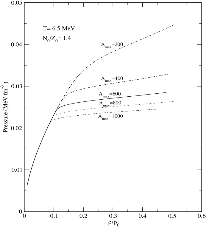
Figure 1: Pressure-density curves for $N_{0}/Z_{0}=1.4$ and $T=6.5$ MeV, where the values of $A_{max}$ used are 200, 400, 600, 800 and 1000. Note that in the region of fast rise of pressure with density results are insensitive to the value $A_{max}$. In the high density side pressure appears to approach a constant value as a function of density as the the value of $A_{max}$ is increased.

We show in Fig.1 $p-\rho$ curves for $N_{0}/Z_{0}=1.4$ where the values of $A_{max}$ are 200, 400, 600, 800 and 1000. The temperature used is $T=6.5$ MeV. For all five choices of $A_{max}$ pressure against $\rho$ initially rises quite sharply and then flattens out considerably. The initial stage of fast rise of pressure with density is the gas phase. Here the results do not matter whether $A_{max}$ is 200, 400 or larger. The reason will become clearer later (it is explained in detail in Chaudhuri1 ). The flattening which follows depend on $A_{max}$ but above a large enough value of $A_{max}$ will not change. For one kind of particles this is reached around 2000 Chaudhuri1 . However, the choice of $A_{max}$=600 is good enough for at least a semi-quantitative estimate of various thermodynamic properties of nuclear matter and we will present results for this value although we did some calculations with other choices of $A_{max}$ also. The flattening happens slightly beyond $\rho/\rho_{0}$=0.1. We show results up to $\rho/\rho_{0}=0.5$ arguing that the excluded volume correction for interactions between composites becomes worse with increasing density.

The rise of pressure at small density followed by a flattening of $p$ with increasing density is a signature of first-order liquid-gas transition. We have shown results for T=6.5 MeV. Beyond a certain temperature the flatness will disappear showing that there is no more phase transition in the domain $\rho/\rho_{0}\leq 0.5$. Similarly the flattening of $p$ disappears beyond some value of $N_{0}/Z_{0}$. The liquid-drop parameters we are using give us for large nuclei the drip-line at $N/Z$ (and of course $Z/N$) about 2. Hence for larger values of $N_{0}/Z_{0}$ the system can not stay together even at $T$=0. Then we will have a system which has a bound core but always many free nucleons which will dominate the thermodynamic properties of the system. This is not a system we want to study. Hence in this work we constrained ourselves to system whose $N_{0}/Z_{0}$ spans 1.0 to 1.8. The upper limit is indeed a highly asymmetric system.

Below the density where phase transition sets in, the system is in pure gas phase. At phase transition point some liquid will be formed and the fraction of nucleons in the liquid phase will grow at the expense of the gas particles as the density increases. This can actually be followed. One also gets a functional definition of what constitutes the gas particles. Here our identification is very different from what is concluded in De1 but very similar to what is found in our earlier work with one kind of particles Chaudhuri1 .

Lastly, in one component model there is just one $\mu$ which stays constant throughout the co-existence region. Now there are two chemical potentials $\mu_{n}$ and $\mu_{p}$. How do they behave?

IV What constitutes the gas and what constitutes the liquid?

The quantity $<n_{A}>\equiv\sum_{N+Z=A}<n_{N,Z}>$ is the average number of composites with mass number $A$. The quantity $A<n_{A}>/A_{0}$ gives the fraction of particles tied up in composites with mass number $A$. This is plotted in Figs.2 and 3 for $N_{0}/Z_{0}$=1.0 and $N_{0}/Z_{0}$=1.8 respectively. First concentrating on Fig.2 (T=6.5 MeV) we see that at density $\rho/\rho_{0}$=0.1 the nucleons are bound in composites $\leq$50. These particles constitute the gas phase. At density $\rho/\rho_{0}$ =0.3 some heavy composites with $A\approx A_{max}$ begin to form and the probability of such heavy particles (with $A$ between $A_{max}$ and $A_{max}$-100) begins to increase (at the expense of the light particles) as the density increases. This is a clear evidence of co-existence. We thus consider light particles ($A\leq 70$) to be gas and heavier particles (with $A$ between $A_{max}$ and $A_{max}$-135) to be liquids. Fig.3 displays similar physics but for $N_{0}/Z_{0}$=1.8 : all gas particles at $\rho/\rho_{0}$=0.1 and mixture of gas and liquid at $\rho/\rho_{0}$=0.38.

We note that even the gas phase in fragmentation model is quite complicated. It is not just neutrons and protons but other light nuclei as well. In addition, during co-existence the isotopic content of the gas phase changes continuously as the volume of the container, i.e. density $\rho/\rho_{0}$ changes. This is called isospin fractionation and is well-known in literature. We will briefly come back to this aspect later.

V Chemical Potentials

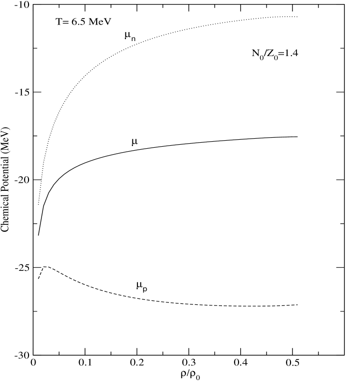
Figure 4: Plot of chemical potential as function of density for $N_{0}/Z_{0}=1.4$ and $T=6.5$ MeV. The dotted line is the neutron chemical potential $\mu_{n}$, the dashed line is the proton chemical potential $\mu_{p}$ and the solid line is $\mu=\frac{N_{0}}{A_{0}}\mu_{n}+\frac{Z_{0}}{A_{0}}\mu_{p}$.

In numerical work involving one kind of particles only Chaudhuri1 it was demonstrated that in the limit of $A_{max}\rightarrow\infty$ a constant value of $\mu$ will be achieved in the co-existence region. This value could be obtained by extrapolation. In the present case there are two chemical potentials. For $N_{0}/Z_{0}\neq 1$, $\mu_{n}\neq\mu_{p}$. For $N/Z$=1.4 and temperature 6.5 MeV we show in Fig.4 the evolution of $\mu_{n}$ and $\mu_{p}$ as a function of density. One notices that both $\mu_{n}$ and $\mu_{p}$ change rapidly in the gas phase and then tend to a constant value. In the limit $A_{max}\rightarrow\infty$ we expect they will become constants. We also plot in the same figure $\mu\equiv\frac{N_{0}}{N_{0}+Z_{0}}\mu_{n}+\frac{Z_{0}}{N_{0}+Z_{0}}\mu_{p}$. The $\mu$ so defined has a meaning at the three limits:-1, 0 and +1 for asymmetry parameter $\omega=\frac{N_{0}-Z_{0}}{N_{0}+Z_{0}}$ and it is interesting to note that $\mu$ tends to constant value faster than either $\mu_{n}$ or $\mu_{p}$.

VI Co-existence Lines

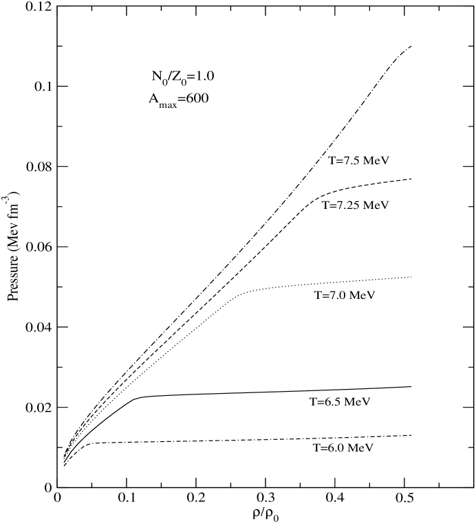
Figure 5: Pressure-density isotherms at $T$=6, 6.5 ,7.0, 7.25 and 7.5 MeV for $N_{0}/Z_{0}=1.4$ and $A_{max}=600$. Note that the point of the beginning of co-existence moves up and to the right as the temperature increases.

Figure 5 shows that as the temperature increases phase co-existence finally disappears (from the region $\rho/\rho_{0}\leq 0.5$). We have shown this for $N_{0}/Z_{0}$=1.0 but this is also true for asymmetric systems provided the asymmetry is not too large as explained earlier.

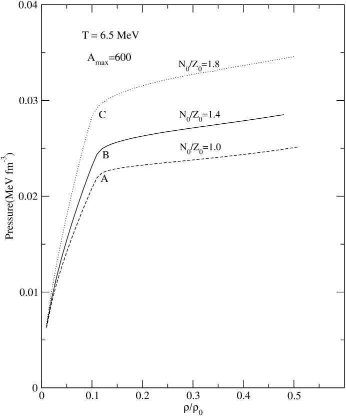
Figure 6: Pressure-density curves at $T=6.5$ MeV for three systems with $(N_{0}/Z_{0})$ values equal to 1, 1.4 and 1.8. The points marked A, B and C on the isotherms will give the values of pressure when co-exsistence sets in at $T=6.5$ MeV for these $N_{0}/Z_{0}$ values.

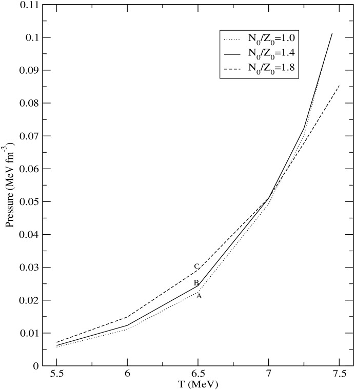
Figure 7: Phase-coexistence lines in the $p-T$ plane for different values of $N_{0}/Z_{0}$. As in Fig. 6 the points marked A, B and C gives the value of pressure where co-existence sets in at $T$=6.5 MeV.

We show in Fig.6 the $p-\rho$ curves at $T$=6.5 MeV for three systems with $N_{0}/Z_{0}$=1, 1.4 and 1.8. We can identify from the figure points $A,B$ and $C$ on these curves where co-existence sets in. The values of pressure at these points give us $p$ values for co-existence at this temperature for these $N_{0}/Z_{0}$ values.. This is not strictly correct. The values of $p$ increase slightly as one moves towards higher density. This is because with $A_{max}$=600 we have not reached asymptotic limits yet. However, this is adequate for our purpose. Repeating this analysis for different temperatures we get co-existence lines in $T-p$ plane for nuclear matter with different asymmetries (Fig.7). Notice that while the co-existence lines for differing asymmetries are different they are quite similar. As usual, points to the left and above the co-existence lines are in the liquid phase and points to the right and below are in the gas phase.

The highest point of a co-existence line in the $T-p$ plane usually identifies critical values $T_{c},p_{c}$ Reif . This is not true in Fig.7. As we consider higher temperatures, points A, B and C (Fig.6) will move to the right and up. They will reach the $\rho/\rho_{0}=0.5$ line. These define the end-points $T,p$ in Fig.7. We do not continue to higher densities as the simple approximation of excluded volume as a means of incorporating interactions between clusters becomes progressively worse. If we accept the validity of the simple multifragmentation model in the region $\rho/\rho_{0}\leq 0.5$ we will have to conclude that the critical point does not exist in the region $\rho/\rho_{0}\leq 0.5$. The same conclusion can be guessed from other published work. Multifragmentation with one kind of particles was also studied by Bugaev et al Bugaev . This is the same physics problem as considered in Chaudhuri1 but treated in a different mathematical framework and these authors considered all densities, not just $\rho/\rho_{0}\leq 0.5$. They found that one can identify a critical point at $T=T_{c}=18.0$ MeV, $\rho/\rho_{0}=1$ and $p_{c}=\infty$. At very high pressure the model must break down but this is an additional confirmation that the simple multifragmentation model in the domain $\rho/\rho_{0}\leq 0.5$ does not contain the critical point.

VII Isothermals in a two-component system

Figure 6 gives the isothermals for $N_{0}/Z_{0}$=1, 1.4 and 1.8 at 6.5 MeV temperature. Drawing isothermals for fixed $N_{0}/Z_{0}$ is physically relevant. We are assuming that we have a very large system with given numbers $N_{0}$,$Z_{0}$ whose volume can change depending upon the physical conditions it is subjected to. If we want to study a different asymmetry we change $N_{0}/Z_{0}$ accordingly and repeat the calculation. To have a complete knowledge, calculations should be done for all relevant $N_{0}/Z_{0}$. The most asymmetric system we study is $N_{0}/Z_{0}$=1.8. Of course, since we have no Coulomb force the system with $N_{0}/Z_{0}=\alpha$ has the same thermodynamic properties as the system with $Z_{0}/N_{0}=\alpha$.

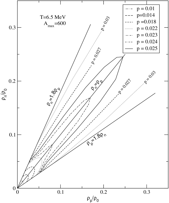
Figure 8: Contours of constant pressure $p$ in $\rho_{n},\rho_{p}$ plane at $T=6.5$ MeV for $A_{max}=600$. The values of the pressure (in MeV/fm³) are marked against the contours and some are given in the box in the upper right corner. The region is bounded by $\rho_{n}=1.8\rho_{p}$, $\rho_{p}=1.8\rho_{n}$ and $(\rho_{n}+\rho_{p})/\rho_{0}\leq 0.5$. The line $\rho_{n}=\rho_{p}$ is shown in the middle.

It is however instructive to consider isothermals of two-component systems in a more general fashion. In a one-dimensional system there is only one density and an isotherm is a line in the $p-\rho$ plane. Now we have two densities $\rho_{n}$ and $\rho_{p}$ and isothermals become surfaces. Let $\rho_{p}$ be the x-axis, $\rho_{n}$ the y-axis and $p$ the z-axis, the equation of state at a given temperature is a surface in this space. A projection of this surface in two dimensions can be made but for a quantitative study it is more convenient to present contours of constant $p$ in $\rho_{p},\rho_{n}$ plane. Such a plot is shown in Fig.8. We consider pressure contours in the region bounded by $\rho_{p}=1.8\rho_{n},\rho_{n}=1.8\rho_{p}$ and $(\rho_{n}+\rho_{p})/\rho_{0}\leq 0.5$. The reasons for choosing these boundaries were explained before.

Roughly speaking, the contours are either largely radial or circular. Let us first consider an uninteresting gas. We assume it consists of only neutrons and protons and unlike in the present problem does not form composites. In such a case constant pressure curves would be $\rho_{n}+\rho_{p}$=constant and these would be straight lines making angle of $\pi/4$ with the x and y axes. Instead we see at low $\rho_{n}$ and $\rho_{p}$ (when one has a gas phase only) not straight lines but more like concentric circles. This is because pressure is directly proportional to multiplicity (section III) and multiplicity is a function of asymmetry. In our case, composites are present in the gas phase and the number of composites depend upon the asymmetry of the system. This causes constant pressure contours in the gas phase to bend from straight lines. We skip the details why the lines become like circles. We now try to explain other pressure contours which are largely radial. For this, refer back to Fig.6. We have mentioned before that in the limit $A_{max}\rightarrow\infty$ the $p-\rho$ curves would have zero slopes to the right of points A, B and C on the isothermals. In such a case constant pressure contour would move exactly radially inwards from the boundary $\rho/\rho_{0}=0.5$, would later leave the radial pattern, bend and finish at the boundary $\rho_{n}=1.8\rho_{p}$ or $\rho_{p}=1.8\rho_{n}$ whichever is appropriate. Similar behaviour is seen in Fig.8. Thus radial pressure contours reflect regions of co-existence.

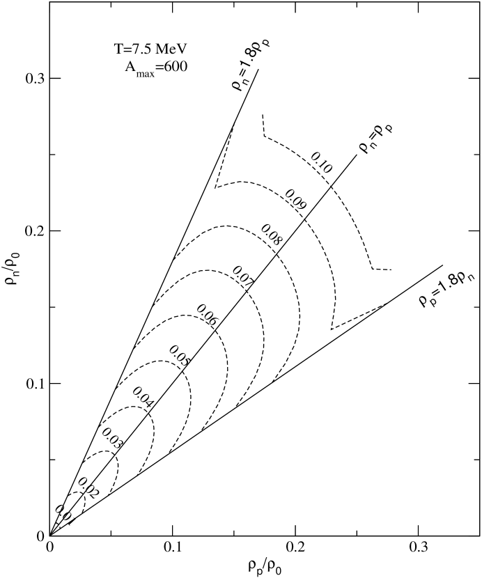
Figure 9: Same as in Fig. 8 except that the temperature is 7.5 MeV. The system is mostly in the gaseous phase which changes the shape of the contours here as compared to that in Fig. 8.

As another example we show in Fig.9 the pressure contours at $T$=7.5 MeV. Except near the edges of the boundaries, pure gas phase is seen.

VIII Isospin Fractionation

We illustrate isospin fractionation in multifragmentation model through an example. Consider multifragmentation of a neutron rich system: $N_{0}/Z_{0}$=1.4 and temperature $T$=6.5 MeV. At low density the system is in pure gas phase. Following section IV, the gas phase consists of light particles with $A\leq 70$ and the liquid phase consists of particles with $A$ between $A_{max}$-70 and $A_{max}$. At higher density, both gas and liquid phases are seen (Figs. 2 and 3). In the present example with $N_{0}/Z_{0}$=1.4, we expect that during co-existence the neutron to proton ratio in the gas phase will rise above 1.4 and the neutron to proton ratio in the liquid phase will fall below 1.4. The reason for this is the symmetry energy which preferentially favours formation of larger clusters closest to maximum stability (i.e.,$N=Z$). This rise of neutron to proton ratio in the gas phase is illustrated in Fig.10. Co-existence sets in a little beyond $\rho/\rho_{0}$=0.1. Till that point is reached the neutron to proton ratio in the gas phase is at 1.4, the ratio of the parent system. Then as the density increases the ratio increases.

Fig.10 also shows that even at very low density the ratio of unbound single neutrons to unbound single protons rises very rapidly. But this has got nothing to do with what is called isospin fractionation. In fact nothing special happens to this ratio when co-existence sets in. It is only if the gas phase is considered to be not just single nucleons but includes light particles as well that isospin fractionation becomes an order parameter if $N_{0}/Z_{0}\neq$ 1.

In the present example, at $\rho/\rho_{0}=0.35$ the neutron to proton ratio in the gas phase is 1.485. In the liquid phase it is 1.375.

Isospin fractionation in mean-field theories is treated in Muller ; Ducoin . Calculations in the lattice gas model can be found in Chomaz1 .

IX Summary

The multifragmentation model, so useful for fitting experimental data in intermediate energy collisions, leads naturally to a model of phase transition for nuclear matter. In a range of temperature and density first order phase transition occurs. The gas phase and the liquid phase can be clearly identified. This is really remarkable. The model of nuclear multifragmentation may be unique in this respect. The gas phase consists of light nuclei with $A$ up to about 70. Besides these gas particles, there are large blobs of matter (liquid) with mass numbers close to $A_{max}$ with $A_{max}\rightarrow\infty$. The model is appropriate at subnormal nuclear density. Modifications of the simple model are needed to extend the model to higher density but this may not be easy.

Actual nuclear systems as created in heavy ion collisions are finite and in addition have Coulomb forces. This makes identification of signals which are finger prints of phase transition difficult. This continues to be the subject of intense study and there is large volume of literature but this is outside the scope of the present article.

X Acknowledgement

This work is partially supported by the Natural Sciences and Engineering Research Council of Canada. Work reported in section VII had its origin from discussions with F. Gulminelli during a past collaboration. We acknowledge a communication with S. Samaddar. We acknowledge generous help from J. Gallego for computation.

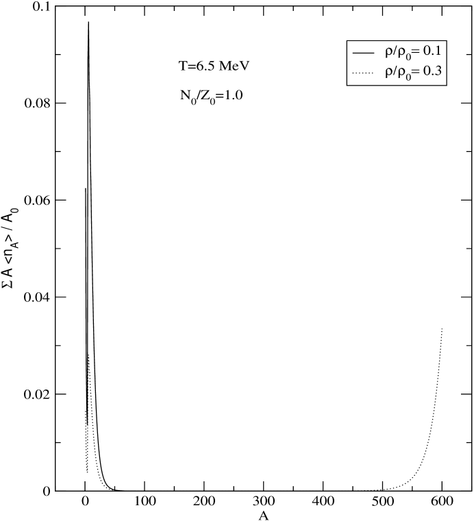
Figure 2: Plot of $A<n_{A}>/A_{0}$ as a function of the mass number A for $N_{0}/Z_{0}=1.0$ and $T$=6.5 MeV. The solid line gives the distribution of composites at $\rho/\rho_{0}=0.1$. There are practically no heavy particles, none above $A$=70. This is pure gas phase. The dotted line is at $\rho/\rho_{0}=0.3$. Now there are both light and heavy ($A\geq 500$) particles. This is co-existence. Here and in the rest of the figures we used $A_{max}$=600.

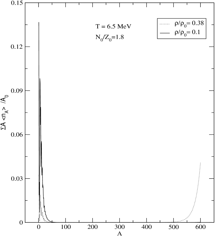
Figure 3: Same as Fig.2 except that it is for $N_{0}/Z_{0}=1.8$ and the dotted line is for $\rho/\rho_{0}=0.38$.

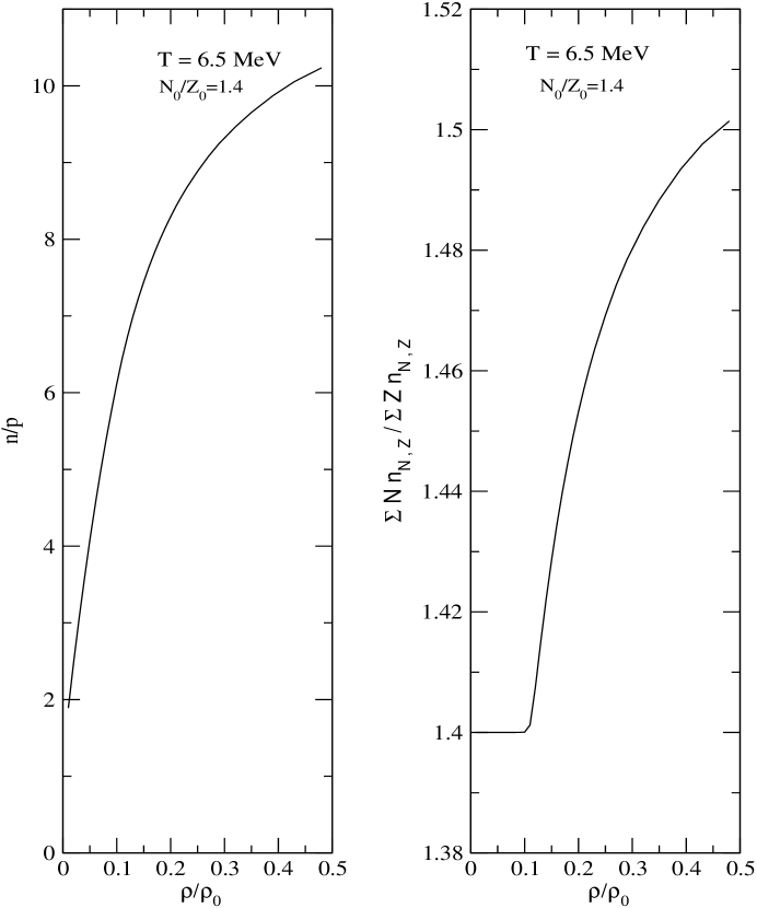
Figure 10: This figure is for $T$=6.5 MeV and $N_{0}/Z_{0}=1.4$. The left panel shows the rise of the ratio of the number of free neutrons to the number of free protons as a function of density. While the rise is fast, nothing particularly new happens at the onset of co-existence. If, however, the gas phase is defined to be all particles with $A\leq 70$ (this would be consistent with Figs 2 and 3), the ratio of neutrons to protons bound in the gas phase remains that of the parent system till co-existence sets in (right panel) and then begins to rise. It behaves like an order parameter if the parent system is asymmetric.

References

- (1) P. Bhattachayya, S. Das Gupta and A. Z. Mekjian, Phys. Rev. C60,064625(1999).
- (2) G. Chaudhuri, S Das Gupta and M. Sutton, Phys. Rev. B74,174106(2006).
- (3) J. N. De and S. Samaddar, Phys. Rev. C76,044607(2007).
- (4) H. Muller and B. Serot, Phys. Rev. C522072(1995)
- (5) C. Ducoin, Ph. Chomaz, and F. Gulminelli, Nucl. Phys A77168(2006)
- (6) S. Das Gupta and A. Z. Mekjian, Phys. Rep. 72, 131(1981).
- (7) C. B. Das, S. Das Gupta, W. G. Lynch, A. Z. Mekjian and M. B. Tsang, Phys. Rep. 406,1,(2005)
- (8) J. P. Bondorf, A. S. Botvina, A. S. Iljinov, I. N. Mishustin and K. Sneppen, Phys. Rep. 257, 133 (1995).
- (9) A. Botvina, G. Chaudhuri, S. Das Gupta and I. Mishustin, Phys. Lett. B668,414(2008)
- (10) F. Reif, Fundamentals of statistical and thermal physics (McGraw Hill, New York, 1965), chap. 8.
- (11) K. A. Bugaev, M. I. Gorenstein, I. N. Mishustin and W. Greiner, Phys. Rev. C 62, 044320 (2000).
- (12) Ph. Chomaz and F. Gulminelli, Phys. Lett B447, 221 (1999)