Computation of the string tension in four-dimensional Yang-Mills theory using large $N$ reduction

Abstract

Continuum reduction and Monte Carlo simulation are used to calculate the heavy quark potential and the string tension in large $N$ Yang-Mills theory in four dimensions. The potential is calculated out to a separation of nine lattice units on a lattice with extent six in each direction.

I Introduction

Through dimensional transmutation, the dimensionless classical coupling constant of QCD is transformed to a running coupling controlled by a physical scale $\Lambda_{QCD}$. Roughly speaking, weak coupling perturbative approximations to processes with momentum transfer $Q$ are expansions in $1/ln(Q/\Lambda_{QCD}$). This gives excellent results when $Q/\Lambda_{QCD}$ is large. When one cannot rely on that, an alternative is the large $N$ approach. The gauge group is generalized to $SU(N)$, and the expansion is in $1/N$.

Although the large $N$ limit of Yang-Mills theory is still out of reach, it is known that it enjoys several simplifications. Among them is the possibility of reducing the space-time volume without affecting certain physical results ek . Continuum reduction nn1 ; knn2 , i.e. reduction to a physical size of order $1/\Lambda_{QCD}$ avoids some of the difficulties bhn ; bs ; tv with reduction to a single space-time point. The addition of double trace terms to the action unsal is an alternative approach.

It is now practical to obtain good results by combining continuum reduction with numerical simulations needing only modest resources. In previous numerical work nn2 ; nn3 ; kn3d ; kn3ds , it has been shown that not only bulk quantities but also physical quantities based on Wilson loops are accessible. The previous results based on Wilson loops have been in three dimensions. In the work described here, we show that the method is still practical in four dimensions.

We have used continuum reduction and Monte Carlo simulation to calculate the heavy quark potential and the string tension in large $N$ Yang-Mills theory in four dimensions. An important aspect of the method is that reduction allows the calculation of infinite volume, infinite $N$ Wilson loops that are larger than the reduced lattice. In particular, in this work, the heavy quark potential is calculated out to a separation of nine lattice units on a lattice with extent six in each direction. The results for the string tension are compatible with those obtained on large lattices at smaller $N$.

II Methods

The standard Wilson Yang-Mills action with gauge group $SU(N)$ is used. In the large $N$ limit, $g^{2}$ is taken to zero with the inverse ’t Hooft coupling $b=\frac{1}{g^{2}N}$ held fixed.

We report results with $N=37$, $47$, and $59$ on a lattice of size $6^{4}$. This is large enough so that in the range of available $b$, the lattice is not too coarse but is still small enough to give a manageable computational cost.

In four dimensions, the useful range of couplings and physical lattice spacings $a$ on a given lattice is more limited than in three dimensions. For $6^{4}$, the system becomes unstable to the bulk transition for small $b$. The smallest $b$ we have used is 0.3450, which is just above the unstable point. For sufficiently large $b$, the center symmetry breaks in one lattice direction, and reduction no longer holds in that direction. This is the large $N$ limit of the finite temperature phase transition knn2 ; jk . For $6^{4}$ it occurs at about $b=0.3515$. Our calculations are at $b=0.3450$, $0.3480$, and $0.3500$ with most of the results at $0.3480$. As measured by the critical size for the finite-temperature transition, that is a range from about $L_{c}=4.4$ to $5.6$. Thus the possibilities for testing scaling are quite limited. For this lattice size, this entire useful range of $b$ is in the region that is metastable to the bulk transition. Nevertheless, we encountered no bulk transitions during the simulations.

As described in previous work knn2 , we update the gauge field configurations with heat bath and over-relaxation methods. In this work, one update will mean one heat bath sweep followed by one over-relaxation sweep. Measurements of the Wilson loops were separated by ten updates. The values for the Wilson loops are based on 1200 measurements.

The measurements of Wilson loops are made on smeared configurations. The use of smeared links improves the measurement of Wilson loops. They enhance the overlap of the space-like sides of the Wilson loops with the ground state. This increases the signal relative to the fluctuations and simplifies the $t$ behavior of the loops teper_sm . The smearing is a four-dimensional version of the method used in kn3d . One lattice direction is arbitrarily chosen as the “time” direction. Links in the remaining three spatial directions (but not in the time direction) are smeared. After the Wilson loops in these “time”-space planes are measured, the process is repeated with each of the other lattice directions chosen as “time.”

When smearing the links in spatial directions, only staples in spatial planes are used. One step in the iteration takes one from a set $U^{(i)}_{k}(x_{1},x_{2},t)$ to a set $U^{(i+1)}_{k}(x_{1},x_{2},t)$. Before reunitarization, the weight of $U^{(i)}_{k}(x_{1},x_{2},t)$ is $(1-f)$ while that of each staple is $f/4$. There are two parameters, namely, the smearing factor $f$ and the number of smearing steps $n$. We use $f=0.45$ and $n=5$ so that $\tau=fn=2.25$ and the associated length scale is $\sqrt{\tau}=1.5$. The use of finer smearing steps $f=0.1$, $n=25$ or a larger length scale $f=0.45$, $n=10$ was more costly and did not lead to further improvement.

Data were collected on planar, rectangular Wilson loops of size $k\times j$ with $k$ and $j$ ranging from 1 to 9 and with $j$ the extent in the “time” direction. The $j$ decay of the loops is fit to a simple exponential. To avoid a possible distortion from a combination of smearing and very small error bars at the shortest separation, loops that are $1\times j$ and $k\times 1$ are not included in the fit. The rate of the exponential decay is taken as the static quark potential at the separation $k$. The $k$ dependence of the exponential is fit to obtain the string tension. With all quantities in lattice units, the three parameter potential that is used in the fits is

$$m(k)=\sigma a^{2}k+c_{0}+\frac{c_{1}}{k}$$ (1)

We expect $c_{0}$ to be positive and of order $1/b$ and $c_{1}$ to be negative and of order $1/b$ or O(1).

Errors in all quantities at a fixed $b$ and $N$ are obtained by jack knife with single elimination.

III Results

We have results for $N=47$ at $b$ values of 0.3450, 0.3480, and 0.3500. In addition, there are results for $N=37$ and $N=59$ at $b=0.3480$.

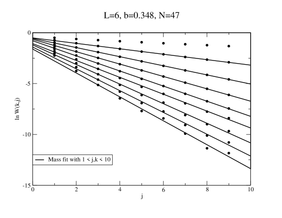
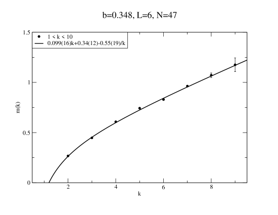
An example of fits to Wilson loop data is given in Fig. 1, which is for $b=0.3480$ and $N=47$. At a fixed $k$, the decay in $j$ of loop data is fit to the form $Ae^{-m(k)j}$ using $k$ and $j$ from 2 through 9, inclusive. This gives the potential $m(k)$ at separation $k$ which is then plotted as a function of $k$ in Fig. 2. A fit of the potential for the $b=0.3480$ and $N=47$ data to the form of Eq. 1 gives

$$\sigma a^{2}=0.099\pm 0.016$$ (2)

To verify that $N$ is sufficiently large, we have the results for $N=37$, $47$, and $59$ in Fig. 3. The string tensions from fits to the $N=47$ and $N=59$ data agree.

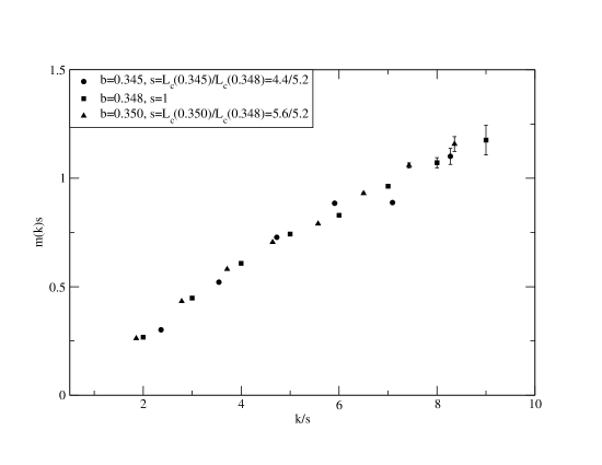
For a check of scaling in the limited range available, we can compare the potentials for $b=0.3450$, $0.3480$, and $0.3500$ all with $N=47$. (For $b=0.3450$, it was necessary to restrict the largest dimension of the loops to 8 to obtain useful fits.) The relative physical scales are set from ratios of the critical lengths $L_{c}(b)$ at which the center symmetry breaks in one direction. These are determined from the results in knn2 . With

$$s(b)=\frac{L_{c}(b)}{L_{c}(0.3480)},$$ (3)

we have $s=4.4/5.2$, $1$, and $5.6/5.2$ for $b=0.3450$, $0.3480$, and $0.3500$, respectively. In Fig. 4, we plot $ms$ verses $k/s$ and see that there is rough agreement of the physically scaled potentials.

IV Conclusion

A comparison with results on large lattices is in order. This can be done by comparing either bare quantities at the same tadpole improved coupling or by comparing a dimensionless ratio. Our result for the string tension in lattice units is $\sigma a^{2}=0.099\pm 0.016$. This is at bare coupling $b=0.3480$ which corresponds to a tadpole improved $b_{I}=b\langle\Box\rangle=0.182$. (The average plaquette $\langle\Box\rangle$ is normalized to approach one in the weak coupling limit.) As it happens, Lucini, Teper, and Wenger ltw1 ; ltw2 have a large lattice, $N=8$ result $\sigma a^{2}=0.116\pm 0.001$ at the same $b_{I}$. This falls within our much larger uncertainty range.

An appropriate dimensionless ratio of physical quantities is $T_{c}/\sqrt{\sigma}$ where, in our case, $aT_{c}=1/L_{c}$. At $b_{I}=0.182$, our result is $T_{c}/\sqrt{\sigma}=0.61\pm 0.05$. After extrapolations to infinite volume, infinite $N$, and zero lattice spacing, Lucini, Teper, and Wenger ltw_1 ; ltw0 ; ltw2 obtain $0.597\pm 0.004$.

In conclusion, we have used large $N$ continuum reduction and Monte Carlo simulation to calculate the heavy quark potential and the string tension in Yang-Mills theory in four dimensions. The results are compatible with those obtained on large lattices at smaller $N$.

Figure 1: Exponential fits to Wilson loops $W(k,j)$ with $j$ on the horizontal axis and $k$ increasing from 1 to 9 going downward.

Figure 2: The static quark potential $m(k)$.

Figure 3: The $N$ dependence of the potential.

Figure 4: Scaling behavior of the potential.