Nonlinear Dynamical Friction in a Gaseous Medium

Abstract

Using high-resolution, two-dimensional hydrodynamic simulations, we investigate nonlinear gravitational responses of gas to, and the resulting drag force on, a very massive perturber $M_{p}$ moving at velocity $V_{p}$ through a uniform gaseous medium of adiabatic sound speed $a_{\rm\infty}$. We model the perturber as a Plummer potential with softening radius $r_{s}$, and run various models with differing $\mathcal{A}=GM_{p}/(a_{\rm\infty}^{2}r_{s})$ and $\mathcal{M}=V_{p}/a_{\rm\infty}$ by imposing cylindrical symmetry with respect to the line of perturber motion. For supersonic cases, a massive perturber quickly develops nonlinear flows that produce a detached bow shock and a vortex ring, which is unlike in the linear cases where Mach cones are bounded by low-amplitude Mach waves. The flows behind the shock are initially non-steady, displaying quasi-periodic, overstable oscillations of the vortex ring and the shock. The vortex ring is eventually shed downstream and the flows evolve toward a quasi-steady state where the density wake near the perturber is in near hydrostatic equilibrium. We find that the detached shock distance $\delta$ and the nonlinear drag force $F$ depend solely on $\mathcal{\eta}=\mathcal{A}/(\mathcal{M}^{2}-1)$ such that $\delta/r_{s}=\eta$ and $F/F_{\rm lin}=(\mathcal{\eta}/2)^{-0.45}$ for $\mathcal{\eta}>2$, where $F_{\rm lin}$ is the linear drag force of Ostriker (1999). The reduction of $F$ compared with $F_{\rm lin}$ is caused by front-back symmetry in the nonlinear density wakes. In subsonic cases, the flows without involving a shock do not readily reach a steady state. Nevertheless, the subsonic density wake near a perturber is close to being hydrostatic, resulting in the drag force similar to the linear case. Our results suggest that dynamical friction of a very massive object as in a merger of black holes near a galaxy center will take considerably longer than the linear prediction.

1 INTRODUCTION

A massive object in orbital motion suffers from orbital decay due to a negative torque caused by gravitational interaction with its own gravitationally induced wake created in the background medium. This process, commonly referred to as dynamical friction (DF), occurs in not only collisionless environments (e.g., Chandrasekhar 1943) but also collisional gaseous backgrounds (e.g., Ostriker 1999). The DF in a gaseous medium is of great importance in understanding the formation and evolution of planets, binary stars, supermassive black holes, etc. For instance, gravitational interaction between a protoplanet and its environmental disk causes the former to migrate toward a central star, naturally explaining the presence of “hot Jupiters” found from radial velocity surveys (Butler et al., 2006, and references therein). The migration also helps a planet grow faster in mass by providing an expanded gas-feeding zone at an enhanced accretion rate, which may overcome the failure of in situ core-accretion scenario in building a giant planet within a typical disk lifetime (see, e.g., Alibert et al., 2005). In the case of nuclear black holes in merging galaxies, they are expected to first experience the DF to form a binary and then coalesce into a supermassive black hole by emitting gravitational waves. Friction of nuclear black holes against the collisionless stellar background appears to be inefficient due to scattering and depletion of stars near the black holes, which is known as the “final-parsec problem” (see Milosavljević & Merritt, 2003, and references therein). However, recent numerical $N$-body/SPH simulations show that the gravitational drag from the gaseous background is sufficient to form a black-hole binary in a relatively short time ($\sim 1-10$ Myrs) (e.g., Escala et al., 2004, 2005; Dotti et al., 2006, 2007; Mayer et al., 2007; Cuadra et al., 2009).

Thanks to a seminal paper of Ostriker (1999), DF in a gaseous medium is well understood as long as density wakes have small amplitudes. Earlier theoretical work by Dokuchaev (1964), Ruderman & Spiegel (1971), and Rephaeli & Salpeter (1980) considered density wakes in a steady state and found that the drag force vanishes for a subsonic perturber, while it becomes remarkably similar to the collisionless counterpart for supersonic cases. Using a time-dependent linear perturbation theory, on the other hand, Ostriker (1999) found that the gravitational drag force on a point-mass perturber with mass $M_{p}$ moving at velocity $V_{p}$ on a straight-line trajectory through a uniform gaseous medium with density $\rho_{\infty}$ and sound speed $a_{\rm\infty}$ is given by

$$F_{\rm lin}=\frac{4\pi\rho_{\infty}(GM_{p})^{2}}{V_{p}^{2}}\left\{\begin{array}[]{ll}\frac{1}{2}\ln(\frac{1+\mathcal{M}}{1-\mathcal{M}})-\mathcal{M},&\mathcal{M}<1,\\ \frac{1}{2}\ln(1-\frac{1}{\mathcal{M}^{2}})+\ln(\frac{V_{p}t}{r_{\rm min}}),&\mathcal{M}>1,\end{array}\right.$$ (1)

where $\mathcal{M}\equiv V_{p}/a_{\rm\infty}$ is the Mach number, $t$ is the time elapsed after the introduction of the perturber, and $r_{\rm min}$ is the minimum radius introduced to avoid the singularity in the force evaluation. Equation (1) shows that the gaseous DF force becomes identical to the Chandrasekhar (1943) formula for the collisionless drag for $\mathcal{M}\gg 1$, and is, albeit small, non-zero even for subsonic perturbers because the time dependency breaks the symmetry in the density wakes (see also Just & Kegel 1990). Equation (1) has been applied to various astrophysical situations including orbital decay of compact objects in accretion disks (e.g., Narayan 2000; Karas & Šubr 2001) and heating of an intracluster medium by supersonically moving galaxies in clusters (e.g., El-Zant et al. 2004; Faltenbacher et al. 2005; Kim et al. 2005; Kim 2007; Conroy & Ostriker 2008).

While the result of Ostriker (1999) is valid in a strict sense only for a linear-trajectory perturber in a uniform medium, it has proven to be applicable to more general cases. For example, Kim & Kim (2007) considered a circular-orbit perturber with orbital radius $r_{p}$ in a uniform gaseous medium and found that equation (1) is a reasonable approximation to the gaseous drag force on it, provided $V_{p}t=2r_{p}$. Sánchez-Salcedo & Brandenburg (2001) numerically found that the orbital decay of a Plummer sphere with a softening radius $r_{s}$ in a radially-stratified medium is consistent with the prediction of equation (1), if $V_{p}t/r_{\rm min}=(0.35r_{p}/r_{s})^{2.34}$. Also, Barausse (2007) showed that equation (1) remains valid even for a perturber with relativistic speed if the relativistic correction factors are included. While Dotti et al. (2006) found that the orbital decay of black hole binaries took longer than the prediction of equation (1) for a single perturber, the discrepancy between the numerical and analytical results can be reconciled, at least partly, by taking allowance for fact that an object in a binary experiences not only a negative torque due to its own wake but also a positive torque from the companion wake. For an equal-mass binary, Kim et al. (2008) found that the positive torque is on average about 40% of the negative torque.

Since the results of Ostriker are based on the assumption that density wakes remain in the linear regime, the validity of equation (1) for very massive perturbers has yet to be seen. The strength of gravitational perturbations due to a body with mass $M_{p}$ can be measured by the dimensionless parameter

$$\mathcal{A}=\frac{GM_{p}}{a_{\rm\infty}^{2}r_{s}},$$ (2)

which roughly corresponds to the perturbed density at a distance $r_{s}$ from the perturber relative to the background density (e.g., Just & Kegel 1990; Ostriker 1999), and is equal to the Bondi radius $r_{\rm B}=GM_{p}/a_{\rm\infty}^{2}$ relative to $r_{s}$. For systems with $\mathcal{A}\gg 1$, the density wakes are clearly in the nonlinear regime and the linear perturbation analyses are likely to fail. Identifying $r_{s}$ with the gravitational softening radius of a perturber (or, equivalently, its size), $\mathcal{A}$ is in the ranges of $\sim 0.1-1$ for galaxies embedded in typical intracluster media, $\sim 10-100$ for protoplanets in protostellar disks, and $\sim 10^{6}-10^{8}$ for supermassive black holes near galaxy centers, suggesting that the wakes of massive compact objects can readily be nonlinear. Indeed, Escala et al. (2005) reported that the orbital decay time of supermassive black hole binaries with $\mathcal{A}\sim 10-100$ depends on $M_{p}$ much less sensitively than the results of the linear theory, which may be caused primarily by the nonlinear effects.

In this paper, we investigate nonlinear DF of a very massive perturber in a gaseous medium using numerical hydrodynamic simulations. In order to isolate the effects of the perturber mass and its velocity on the DF force, we consider a perturber following a straight-line trajectory in a uniform gaseous medium, similarly to in Ostriker (1999). We model the perturber as a Plummer sphere that does not possess any solid surface and merely provides gravitational potential perturbations to the background medium that would otherwise remain static and uniform; to make contact with the results of the linear theory, we ignore the accretion of gas onto the perturber in the current work. Our primary objectives are to find the changes in distributions of density wakes with $\mathcal{A}$ and $\mathcal{M}$, and to quantify the resulting gravitational drag forces in comparison with the linear cases.

Nonlinear responses of a background to a massive perturber moving at a supersonic speed have been extensively studied in the context of the Bondi-Hoyle-Lyttleton (BHL) accretion (Hoyle & Lyttleton 1939; Bondi & Hoyle 1944; Bondi 1952; see also review of Edgar 2004 and references therein). Unlike our models where mass accretion to a perturber is prohibited, however, the BHL accretion problem considered a perturber containing a defined surface through which gas is either accreted or reflected. It was Hunt (1971, 1979) who first solved for BHL accretion flows numerically, finding that the collisional nature of gas supports a bow shock in front of a supersonic perturber. Later studies found that the BHL accretion flows exhibit unstable behaviors such as flip-flop motions of the accretion shocks and vortex shedding when the condition of axisymmetry is relaxed (e.g.,Matsuda et al. 1987; Fryxell & Taam 1988; Taam & Fryxell 1988; Matsuda et al. 1989; Ruffert 1994; Foglizzo & Ruffert 1997, 1999; Foglizzo et al. 2005). While these numerical works on the BHL accretion explored temporal evolution and distribution of density wakes as well as nonlinear features in some great detail, they mainly concentrated on the gravitational focusing and resulting accretion rate of gas onto the perturber. Although some authors (e.g., Shima et al. 1985; Shankar et al. 1993; Ruffert 1996) presented values for aerodynamic and gravitational drag forces, only a limited range of $\mathcal{A}$ was covered. In this work, we run a number of numerical simulations by varying $\mathcal{A}$ and $\mathcal{M}$ systematically in order to quantify the dependences of the gravitational drag force on these parameters. A brief comparison between our results with those from the BHL accretion studies will be presented.

This paper is organized as follow: In §2, we describe numerical methods we employ for nonlinear simulations. In §3, as a code test we revisit the cases with a spatially-extended, linear perturber with $\mathcal{A}=0.01$. We compare the resulting distributions of density and velocity wakes with those of analytical results and provide a way to handle the effect on the DF force of a softening radius which is necessary for numerical simulations. Evolution and quasi-steady distributions of fully nonlinear density wakes and the associated drag forces are presented in §4. Finally, in §5 we summarize our findings and discuss their astrophysical implications.

2 NUMERICAL METHOD

In this paper, we consider an unmagnetized, inviscid, non-radiating, non-self-gravitating gaseous medium and study its gravitational responses to a massive perturber moving along a straight-line trajectory using numerical simulations. The background gaseous medium is initially static and uniform with density $\rho_{\infty}$ and adiabatic sound speed $a_{\rm\infty}$. We adopt an adiabatic equation of state with an index $\gamma=5/3$ throughout simulations. The simulations are carried out on a two-dimensional $(R,z)$ plane in cylindrical symmetry, where $R$ and $z$ denote the distances from and along the axis of symmetry, respectively. We assume that the perturber exerts only gravity to the surrounding medium and does not possess any surface, so that neither accretion nor reflection of the gas is allowed. The perturber is modeled as a Plummer sphere with mass $M_{p}$ that is moving at a constant speed $V_{p}$ along the $R=0$ axis toward the positive $z$-direction, with the gravitational potential

$$\Phi_{P}(R,z,t)=-\frac{GM_{p}}{(R^{2}+r_{s}^{2}+[z-V_{p}t]^{2})^{1/2}},\;\;\;{\rm for}\;t\geq 0,$$ (3)

where $r_{s}$ is the softening radius.

We take $r_{s}$, $a_{\rm\infty}$, and $t_{\rm cross}=r_{s}/a_{\rm\infty}$ as the units of length, velocity, and time, respectively, in our simulations. Then, our models are completely parametrized by $\mathcal{A}$ and $\mathcal{M}$. We run a total of 58 models with $\mathcal{A}$ varying from 0.01 to 600 and $\mathcal{M}$ in the range of 0.5 to 4.0. We solve the basic equations of ideal hydrodynamics using FLASH3 (Fryxell et al., 2000), an Eulerian hydrodynamics code that implements a direct Piecewise-Parabolic Method solver of Colella & Woodward (1984) for high-order spatial reconstruction. Although the FLASH3 code is capable of both uniform grid and adaptive mesh refinement calculations, we adopt the uniform grid method since the accurate evaluation of the drag force requires the whole computational domain to be well resolved. As we will show below, we find that it is necessary to have at least 5 zones per $r_{s}$ to obtain converged results for the drag forces. Our largest grid models have 3,072$\times$12,288 zones in $(R,z)$; we make sure that our computational domain is taken to be large enough to contain the whole density wake in a given model. The simulations are typically carried out until $t/t_{\rm cross}=600$ when most of the wakes are well resolved and reach a quasi-steady state.

3 LINEAR CASES

Time-dependent linear perturbation theories for the DF drag force in a gaseous medium usually study the responses of gas to a low-mass, point-mass perturber corresponding to $r_{s}=0$ in the Plummer potential (e.g., Just & Kegel 1990; Ostriker 1999), which requires to introduce the cut-off radius $r_{\rm min}$ in the linear force formula (eq. [1]). In numerical simulations, on the other hand, one needs to assign a non-zero value to the softening radius, which in turn makes it unnecessary to use the cut-off radius in the force evaluation. Since our goal is to compare the nonlinear drag force on a massive perturber with the linear prediction, we have to first find a proper relationship between $r_{s}$ and $r_{\rm min}$ that makes the numerical and analytical results consistent with each other when $A\ll 1$. Motivated by this consideration, in this section we briefly present the results of numerical simulations for a low-mass perturber with $\mathcal{A}=0.01$, and compare the resulting distributions of density and velocity wakes and the drag forces with those from the linear theories. This will also allow us to check the accuracy of our numerical experiments.

Regarding the linear wakes with which numerical results will be compared, it is worth mentioning that there are several analytical methods for finding solutions for the perturbed density and velocity fields. Just & Kegel (1990) utilized Fourier transform for the space variables and Laplace transform for the time variable, finding expressions both for the density and velocity wakes. Instead, Ostriker (1999) used a retarded Green’s function technique and found an expression only for the density wake that is identical to the result of Just & Kegel (1990). We found that while the analytical formula for the density wake agrees well with our numerical results for a low-mass perturber, the simulated velocity field differs from the expression given by Just & Kegel (1990). In Appendix A, we revisit the time-dependent linear theory using Fourier transforms both for the space and time variables. As we will show below, our expressions (A19) and (A20) for the perturbed velocities are in good agreement with the numerical results, confirming that equation (47) of Just & Kegel (1990) contains a typographical mistake.

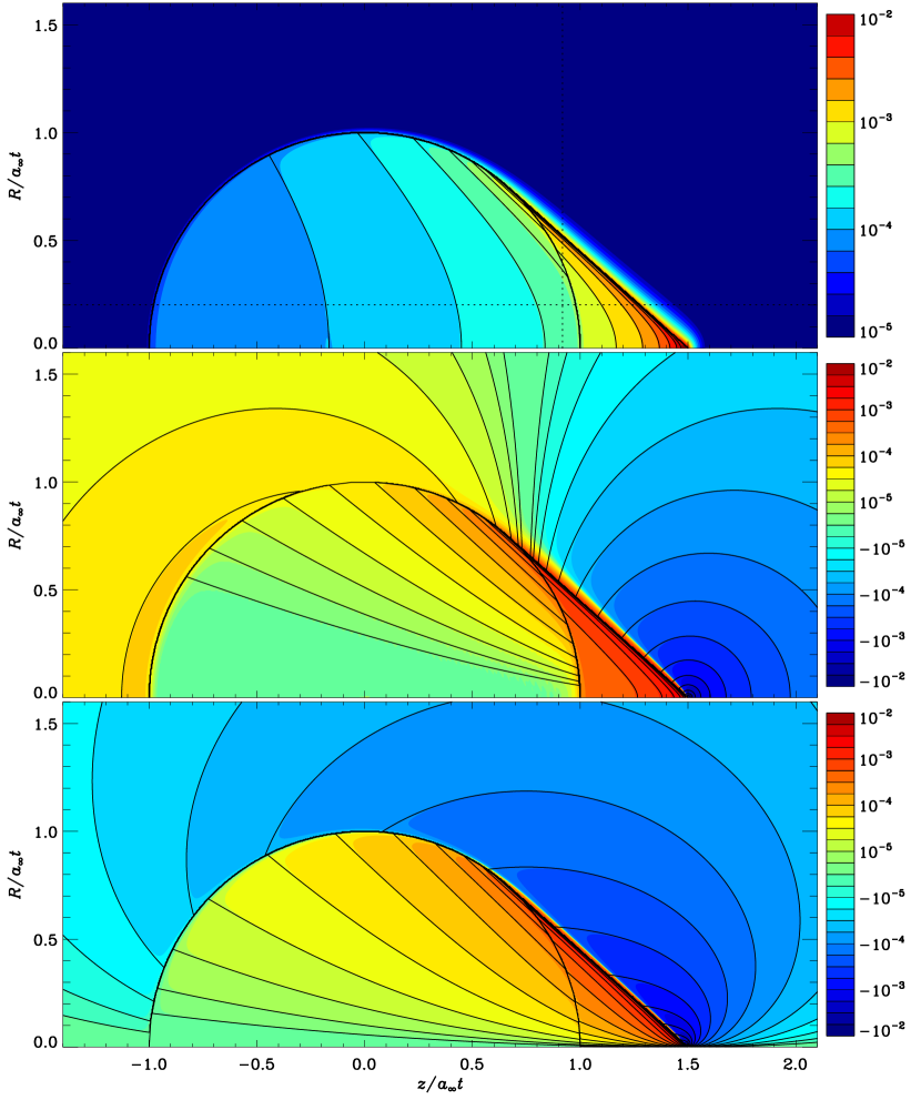
Figure 1: Color-scale distributions of the perturbed density $\alpha$ (top), parallel velocity $v_{z}$ (middle), and perpendicular velocity $v_{R}$ (bottom) to the line of motion of an extended perturber with $\mathcal{A}=0.01$ and $\mathcal{M}=1.5$. Colorbars label $\alpha$, $v_{z}/a_{\rm\infty}$, and $v_{R}/a_{\rm\infty}$ from top to bottom. The black contours represent the results of the time-dependent linear perturbation theory for the corresponding point-mass perturber. The perturber initially located at $(z,R)=(0,0)$ has moved to $(\mathcal{M}a_{\rm\infty}t,0)$ at time $t$ along the $z$-axis.

Figure 1 shows as color-scale images the snapshots on the $z$–$R$ plane of the perturbed density $\alpha=\rho/\rho_{\infty}-1$ (top), the parallel velocity $v_{z}$ (middle), and the perpendicular velocity $v_{R}$ (bottom) to the line of motion for a model with $\mathcal{A}=0.01$ and $\mathcal{M}=1.5$. Note that the coordinates are normalized by $a_{\rm\infty}t$. The perturber initially introduced at $(z,R)=(0,0)$ has moved to $(\mathcal{M}a_{\rm\infty}t,0)$ at time $t$. The characteristic features of a supersonic wake consisting of a sonic sphere with radius $a_{\rm\infty}t$ centered at the initial perturber location and a Mach cone bounded by Mach waves located at $R=-(\mathcal{M}^{2}-1)^{-1/2}(z-\mathcal{M}a_{\rm\infty}t)$ for $z>a_{\rm\infty}t/\mathcal{M}$ are apparent in the top panel. Also plotted as black solid contours are the results of the linear perturbation theory (eqs. [A10], [A19], and [A20]), which are overall in good agreement with the numerical results. A careful inspection of Figure 1, however, reveals that the numerical results deviate slightly from the analytical ones especially near the sonic radius and the Mach waves. This is due to the fact that the perturber in our numerical models is modeled as an extended Plummer sphere rather than a point mass.

One can semi-analytically construct the density wake $\alpha_{\rm ext}$ of an extended perturber by convolving the density wake $\alpha$ due to the corresponding point mass with the extended mass distribution $\rho_{\rm ext}$ of the perturber (e.g., Just & Kegel 1990; Furlanetto & Loeb 2002). For a Plummer sphere we use, the convolution theorem gives

$$\alpha_{\rm ext}(\mbox{\boldmath{$x$}},t)=\frac{1}{M_{p}}\int\alpha(\mbox{\boldmath{$x$}}-\mbox{\boldmath{$x^{\prime}$}},t)\rho_{\rm ext}(\mbox{\boldmath{$x^{\prime}$}},t)\;d^{3}\!\mbox{\boldmath{$x^{\prime}$}},$$ (4)

where $\rho_{\rm ext}(\mbox{\boldmath{$x$}},t)=3M_{p}r_{s}^{2}(R^{2}+r_{s}^{2}+(z-V_{p}t)^{2})^{-5/2}/(4\pi)$. Figure 2 plots as solid lines the profiles of $\alpha_{\rm ext}$ for $\mathcal{A}=0.01$ and $\mathcal{M}=1.5$ along the cuts at $R/a_{\rm\infty}t=0.20$ and $z/a_{\rm\infty}t=0.92$ marked as dotted lines in the top panel of Figure 1, which are in excellent agreement with the simulation outcomes (open circles). Compared with the point-mass results (dashed lines), the extended mass distribution tends to smear out the discontinuities at the boundary of the sonic sphere and the Mach cone. This makes sense since a perturbed density at one location is a superposition of sonic perturbations with various strengths launched by all the mass elements comprising the extended body.

Allowing for the extended mass distribution, the gravitational drag force exerted on the perturber in the negative $z$-direction can be obtained by directly evaluating the integral

$$F(t)=\int\!\!\!\!\int\frac{G\rho_{\rm ext}(\mbox{\boldmath{$x^{\prime}$}},t)\rho(\mbox{\boldmath{$x$}},t)(z-z^{\prime})}{|\mbox{\boldmath{$x$}}-\mbox{\boldmath{$x^{\prime}$}}|^{3}}\ d^{3}\mbox{\boldmath{$x$}}\ d^{3}\mbox{\boldmath{$x^{\prime}$}},$$ (5)

where $\rho(\mbox{\boldmath{$x$}},t)$ is the wake distribution. Although equation (5) requires the $x^{\prime}$-integration to be performed over the entire Plummer sphere, we empirically found that the drag force on the region with distance from the perturber larger than $10r_{s}$ has a negligible contribution to the total. Thus, in practice, we limit the integration to the region within $10r_{s}$ that contains about 98.5% of the total perturber mass. Figure 3 plots as open squares the numerical drag forces on a low-mass perturber with $\mathcal{A}=0.01$ but differing $\mathcal{M}$. The solid line corresponds to equation (1) with

$$r_{\mathrm{min}}=0.35\mathcal{M}^{0.6}r_{s},$$ (6)

which gives the best fit to the supersonic results of our adiabatic simulations. Equation (6) is our prescription for the cut-off radius when we compare the numerical drag forces with the analytic results. Note that Sánchez-Salcedo & Brandenburg (1999) suggested $r_{\rm min}=2.25r_{s}$ based on their isothermal simulations. The difference between the two prescriptions may be due in part to using different equations of state and in part to low resolution (1 cell per $r_{s}$) in Sánchez-Salcedo & Brandenburg (1999).

4 NONLINEAR CASES

4.1 Wake Evolution

4.1.1 Supersonic Cases

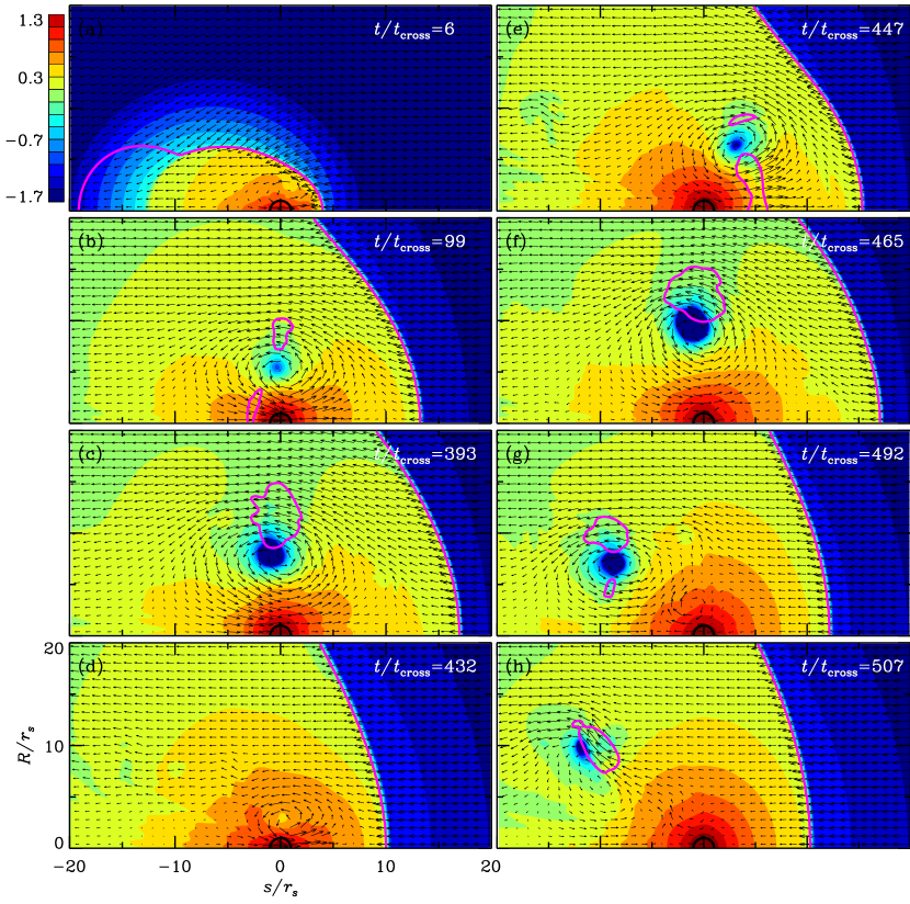
Figure 4: Temporal evolution of the density structure (logarithmic color-scale) and velocity field (arrows) generated by an extended perturber with $\mathcal{A}=20$ and $\mathcal{M}=1.5$ in the frame where the perturber located at $(s=z-V_{p}t,R)=(0,0)$ is stationary. A black semicircle marks the softening radius of the perturber, while red curves draw the sonic lines where the gas speed is equal to the local sound speed. Colorbar labels $\log(\rho/\rho_{\infty}-1)$.

We begin by describing the temporal evolution of our fiducial model with $\mathcal{A}=20$ and $\mathcal{M}=1.5$; the evolution of other supersonic models are qualitatively similar. Figure 4 illustrates the density and velocity structures of this model in a comoving frame with the perturber located at $(s\equiv z-V_{p}t,R)=(0,0)$. Only the region with $|s|/r_{s}\leq 20$ and $0\leq R/r_{s}\leq 20$ is shown. Unlike the linear cases with $\mathcal{A}\ll 1$ where the density wakes have too small amplitudes to launch shock waves, the perturber with $\mathcal{A}=20$ emits strong perturbations that quickly develop into a bow shock. The upstream gas moving toward the perturber along the symmetry axis is first accelerated by the gravity of the perturber, is shocked to subsonic speed, and then piles up near the center of the perturber. This creates a steep pressure gradient in between the perturber and the shock, tending to push the shock away from the perturber. On the other hand, the gas flowing above (not far away from) the symmetry axis is deflected toward the perturber even before entering the shock and decreases its speed after the shock. This gas thus has a longer time to be exposed to the gravity of the perturber as it moves toward the symmetry axis. The gravitational potential is so deep that the material arriving at the rear side of the perturber can be pulled back toward the perturber, creating a stagnation point just as in the BHL accretion flows (e.g., Matsuda et al. 1987; Fryxell et al. 1987). This produces a strong counterstream that moves into the upstream direction along the symmetry axis, as well as a primary vortex in the $s$–$R$ plane (Fig. 4a). The counterstream combined with the pressure gradient in the front side pushes the shock front away from the perturber.

The advance of the shock front in the upstream direction allows more time for the shocked gas to be affected by the gravity, strengthening the counterstream (as well as the primary vortex) and thus increasing the detached distance $\delta$ of the shock measured along the symmetry axis. At the same time, the center of the vortex with a lower density than the surrounding buoyantly rises toward the high-$R$ regions. This decreases the ram pressure of the counterstream exerted on the shock front and the shock advance slows down. Figure 5 plots the time evolution of $\delta$ for some selected models, while Figure 6 traces the trajectory of the center of the primary vortex in our standard model ($\mathcal{A}=20$ and $\mathcal{M}=1.5$) on the $s$–$R$ plane. For our standard model, $\delta$ keeps increasing to $13r_{s}$ at $t/t_{\rm cross}=100$. At this time, the vortex is located near at $(s,R)\simeq(-0.2r_{s},5r_{s})$ (Figs. 4b and 6). The shock front soon overshoots a potential equilibrium position where the thermal pressure of the postshock gas supports it against the perturber gravity, and begins oscillating around the equilibrium position.

The shock oscillation changes the velocity field in the postshock region, causing the vortex to move in the counterclockwise direction around its mean position $(-0.5r_{s},5r_{s})$ following the background flow. Kelvin’s circulation theorem implies that the vortex becomes stronger as it moves toward the symmetry axis, amplifying the strength of the counterstream near the perturber. The velocity of the counterstream becomes largest when the vortex arrives closest to the perturber on its oscillation path (Fig. 4d). The shock front that was moving toward the perturber is pushed by the strong counterstream, and reverses its motion. The vortex rises to high $R$ as the shock moves away from the perturber, weakening the counterstream, and the oscillation cycle repeats quasi-periodically.

Figures 5 and 6 show that the amplitudes of the detached shock oscillations as well as the vortex movements grow secularly with time as the shock oscillation continues. This can be understood as follows. When the shock front is displaced from the equilibrium position away from the perturber (e.g., Fig. 4c), the shocked subsonic gas can acquire an extended time to be gravitationally influenced, similarly to the early situation when the shock advances away from the perturber. With the stagnation point moving away from the perturber, more mass and momentum are added to the counterstream, amplifying the vortex oscillation. In addition, when the strong counterstream collides directly with the shocked subsonic flow near the symmetry axis, the material at the interface is injected upward in the lateral direction and then carried in the negative $s$-direction by the background flow (see, e.g., the region at $s/r_{s}\sim 12$ and $R/r_{s}\sim 0-3$ in Fig. 4e). This produces small vortices near the interface that move downstream and merge with the primary vortex, again strengthening the latter. Consequently, the primary vortex is able to move closer to the symmetry axis and amplify the counterstream in the next cycle, making the shock oscillation overstable.

As the center of the primary vortex moves away from the symmetry axis during its last phase of the overstable oscillation ($t/t_{\rm cross}\sim 465-492$), it becomes less gravitationally bound and can thus be more easily influenced by the background flow. For all the supersonic models we run in this paper, we find that whenever the vortex rises above a half of the accretion radius, also known as the Hoyle-Lyttleton radius, defined by $r_{\rm A}\equiv 2GM_{p}/V_{p}^{2}$, it is swept away by the background flow in the negative $s$-direction (Fig. 6). When the primary vortex is located outside $0.5r_{\rm A}$, the counterstream associated with the vortex is weak and occurs in the far rear side of the perturber, unable to pass through the center of the perturber. The counterstream is instead resisted by the flow moving downstream right across the perturber and pushed up in the lateral direction (Fig. 4g). This develops another vortex with an opposite sense of rotation to the primary one, capable of pushing the latter away from the perturber (Fig. 4h). With the primary vortex carried away downstream, the flow near the perturber reaches a quasi-steady state in which shocked subsonic gas moves almost parallel to the symmetry axis. Since the associated kinetic energy is much smaller than the thermal and gravitational energies of the gas, the density distribution around the perturber becomes nearly hydrostatic, as will be shown below.

4.1.2 Subsonic Cases

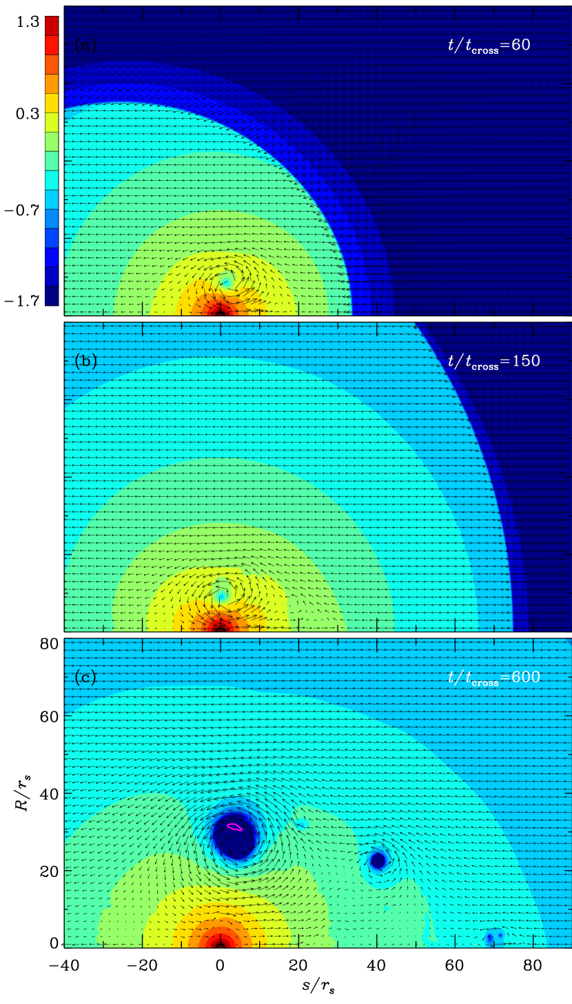
Figure 7: Snapshots of the perturbed gas density (logarithmic color-scale) overlaid with the velocity structure (arrows) of a nonlinear subsonic model with $\mathcal{A}=20$ and $\mathcal{M}=0.5$ in a comoving frame with the perturber. Colorbar labels $\log(\rho/\rho_{\infty}-1)$.

Figure 7 displays density and velocity structures of a nonlinear subsonic model with $\mathcal{A}=20$ and $\mathcal{M}=0.5$ in a comoving frame with the perturber. Snapshots at $t/t_{\rm cross}=60$, 150, and 600 are shown. Sound waves launched from the perturber at $t=0$ propagate radially outward into the surrounding medium, forming a spherical causal region within which the medium is affected by the sonic perturbations. Since the perturber is spatially extended, however, the boundary of the casual region is not as sharp as in the case of a point mass, although the most dominant perturbations still come from the perturber center. Unlike supersonic cases, this model always involves subsonic flows and never produces a shock. Nevertheless, the overall flow pattern and late-time density structure near the perturber of this model is very similar to those in the postshock subsonic regions of supersonic models. First of all, the strong gravitational pull forms a counterstream and an associated vortex ring near the symmetry axis (Fig. 7a). The counterstream moving in the upstream direction interacts with the incident flow (Fig. 7b). The gas at the interface is pushed up toward the high-$R$ regions and then carried downstream, creating small vortices with low density (Fig. 7c).

The primary vortex slowly rises in the $R$-direction due to buoyancy, and merge with the small vortices. Since this model does not contain a shock that would confine the region of influence and since the causal region keeps expanding at a sonic speed, the flows in the high-$R$ regions are almost parallel to the symmetry axis. As a result, the primary vortex keeps rising as there is no momentum input in the background flow capable of pushing it back toward the symmetry axis. At the end of the run ($t/t_{\rm cross}=600$), the primary vortex in this model arrives at $(s,R)=(3r_{s},28r_{s})$, corresponding to $0.18r_{\rm A}$. It is uncertain whether the primary vortex will be carried downstream when it goes beyond $r=0.5r_{\rm A}$ in a manner similar to supersonic cases. At any event, the density distribution close to the perturber is well described by the condition of hydrostatic equilibrium at late time (see §4.2 below).

4.2 Quasi-steady Density Wakes

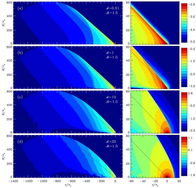
Figure 8: Distributions of quasi-steady density wakes with varying $\mathcal{A}$ on the $s$–$R$ plane at $t/t_{\rm cross}=600$, with the perturber placed at $(s,R)=(0,0)$. Left panels show large-scale views of $\alpha$, while the right panels focus on a small section with $-60\leq s/r_{s}\leq 20$ and $0\leq R/r_{s}<60$ near the perturber. All the models have the same $\mathcal{M}=1.5$. The black line in each panel traces the Mach cone formed by a low-mass point-mass perturber with the same Mach number. The perturber gathers more gas toward it as $\mathcal{A}$ increases. Colorbars label $\log(\rho/\rho_{\infty}-1)$.

Figure 8 illustrates changes in the quasi-steady density wakes with varying $\mathcal{A}$ on the $s$–$R$ plane for supersonic models with fixed $\mathcal{M}=1.5$ at $t/t_{\rm cross}=600$. The left panels show large-scale views of the wakes at $-1400\leq s/r_{s}\leq 100$ and $0\leq R/r_{s}\leq 600$, while the region near the perturber with $-60\leq s/r_{s}\leq 20$ and $0\leq R/r_{s}\leq 60$ is enlarged in the right panels. In each panel, the perturber is located at $s=R=0$, and the black line connecting the points $(s,R)/r_{s}=(0,0)$ and $(-60,54)$ marks the boundary of the Mach cone characteristics of the linear density wake for $\mathcal{M}=1.5$. When $\mathcal{A}\ll 1$, the sonic perturbations are too weak to produce a shock, and the high-density ridge of the wake follows the Mach cone fairly well, although it is broadened due to the extended mass distribution of the perturber. As $\mathcal{A}$ increases to unity, sonic perturbations even outside the Mach cone attain substantial amplitudes enough to induce a bow shock that is attached to the center of the perturber (within the resolution limit). Since the density wake is effectively shifted toward the perturber compared with the linear case and still located preferentially at the rear side of the perturber, the resulting drag force will be larger than the linear counterpart (see §4.4).

As $\mathcal{A}$ increases further, the shocked material gathered around the perturber begins to build up a strong pressure barrier which the incident flow cannot easily penetrate. This naturally makes the shock detached. Figure 8b,c shows that the postshock density distribution around the perturber with $\mathcal{A}=10$ or 20 is almost spherically symmetric, indicating that the kinetic energy of the gas there is much smaller than the thermal and gravitational potential energies. To check if this is indeed the case, we plot in Figure 9 the density profiles along the symmetry axis and the $R$-axis from the center of a massive perturber with $\mathcal{A}=20$; both supersonic and subsonic models with $\mathcal{M}=1.5$ and $0.5$ at $t/t_{\rm cross}=600$ are presented. Also shown as dotted line is the density distribution under the assumption of hydrostatic equilibrium

$$\rho=\rho_{0}\left\{1+\frac{(\gamma-1)\mathcal{A}a_{\rm\infty}^{2}}{a_{0}^{2}}\left[\frac{r_{s}}{(r^{2}+r_{s}^{2})^{1/2}}-1\right]\right\}^{1/(\gamma-1)},$$ (7)

where $r=(s^{2}+R^{2})^{1/2}$ denotes the distance from the perturber center and $\rho_{0}$ and $a_{0}$ are the density and the adiabatic sound speed at $r=0$, respectively.

For both supersonic and subsonic models, the density distributions at $r/r_{s}\lesssim 10$ along the $z^{+}$-, $z^{-}$-, and $R$-cuts are virtually identical to each other, and are in remarkable agreement with the predictions of equation (7) with $\rho_{0}/\rho_{\infty}=40$ and $a_{0}/a_{\rm\infty}=3.8$ for $\mathcal{M}=1.5$, and $\rho_{0}/\rho_{\infty}=52$ and $a_{0}/a_{\rm\infty}=3.8$ for $\mathcal{M}=0.5$. The sharp drop offs of the density in the supersonic model near $r/r_{s}=12$ and $32$ along the $z^{+}$- and $R$-directions, respectively, are of course due to the bow shock. In the subsonic model, the presence of the primary vortex makes the local density decreased at $R/r_{s}=28$. Note that the quantity $a^{2}/\rho^{\gamma-1}$ measures the specific entropy and thus is conserved in an adiabatic flow without involving a shock, as is the case in the subsonic model. For the supersonic model, however, $a^{2}/\rho^{\gamma-1}$ is increased from unity to 1.34 because of a shock jump. This corresponds to the shock Mach number of $2.3$, which is larger than $\mathcal{M}=1.5$ because the flow is accelerated by the perturber even before experiencing the shock. In the regions with $r/r_{s}\gtrsim 10$, the density is overall larger along the $z^{-}$- than $z^{+}$-directions, providing non-vanishing drag forces. Nonetheless, the presence of hydrostatic cores in the density wakes of massive supersonic perturbers makes the drag forces smaller than the linear results.

While the density wake near a massive perturber with $\mathcal{A}\geq 1$ is quite different from the linear counterpart, the distant part of the wake is more or less the same. Figure 10 plots the exemplary profiles of the normalized perturbed density, $\alpha/\mathcal{A}$, along the cuts with $R=0$ and $R/r_{s}=200$ for models shown in Figure 8. Note that $\alpha/\mathcal{A}$ is nearly independent of $\mathcal{A}$ in regions far away from the perturber (e.g., $s/r_{s}<-900$ region in Fig. 10a and $s/r_{s}<-500$ region in Fig. 10b); in these regions, the gravitational potential perturbations are weaker by more than two orders of magnitudes than at the perturber location and thus locally in the linear regime. Even with low amplitudes of local perturbations, however, the region with $-900<s/r_{s}<-100$ along the symmetry axis behind the perturber has the nonlinear density wake that deviates considerably from the linear case. This is because the gas flowing in this region was already affected by strong gravitational potential in the upstream region, and has a diverging velocity field that reduces the perturbed density. Small fluctuations of nonlinear density wakes apparent in Figures 8 and 10 near the $R=0$ axis is thought of as arising from sonic perturbations induced by the primary vortex and its oscillations discussed in §4.1.

4.3 Detached Shock Distance

We have shown in the previous subsection that a sufficiently-massive supersonic perturber generates a density wake that is characterized by a bow shock standing ahead of the perturber and a surrounding hydrostatic envelope. Figure 5 shows that the quasi-steady value of the detached shock distance $\delta$ is larger for models with larger $\mathcal{A}$ or smaller $\mathcal{M}(>1)$. To quantify the dependences of $\delta$ upon $\mathcal{A}$ and $\mathcal{M}$, we introduce the nonlinearity parameter

$$\mathcal{\eta}\equiv\frac{\mathcal{A}}{\mathcal{M}^{2}-1},$$ (8)

and plot in Figure 11 the normalized shock distance against $\mathcal{\eta}$. The various symbols give the mean values of $\delta$ temporally averaged over $t/t_{\rm cross}>50$ that ignores the initial wake-development phase. The standard deviations of $\delta$ are also indicated by errorbars. The numerical results are remarkably well described by the two simple power laws: $\delta/r_{s}=2(\mathcal{\eta}/2)^{2.8}$ for $0.7\lesssim\mathcal{\eta}\lesssim 2$ and $\delta/r_{s}=\mathcal{\eta}$ for $\mathcal{\eta}>2$.

The behavior of $\delta$ with $\eta$ can be qualitatively understood as follows. For a very massive perturber, the kinetic energy of the incident flow along the symmetry axis is almost entirely converted to the thermal energy of the postshock flow that supports a hydrostatic envelope against the gravitational potential of the perturber. When the shock is strong ($\mathcal{M}\gg 1$), the postshock thermal energy proportional to $a_{\rm\infty}^{2}\mathcal{M}^{2}$ balances the gravitational potential energy $-GM_{p}/\delta$ at the shock location, resulting in $\delta/r_{s}\propto\mathcal{A}/\mathcal{M}^{2}$. In the limit of $\mathcal{M}\rightarrow 1$, the flow does not in principle produce a shock, corresponding to $\delta\rightarrow\infty$. In practice, the gravitational acceleration is able to turn an incident nearly-transonic gas into a weakly supersonic flow, but the shock that may form is located very far away from the perturber anyway. In view of the detached shock distance, $\eta$ may be a better indicator of nonlinearity than $\mathcal{A}$; for fixed $\mathcal{A}$, the shape of a density wake due to a supersonic perturber becomes similar to the linear counterpart as $\mathcal{M}$ increases.

It is well known from hydrodynamic experiments and corresponding theories that a supersonic flow over a solid object with a blunt nose develops a detached bow shock when the nose angle is larger than the maximum angle allowed by the postshock flow (e.g., Liepmann & Roshko 1957, and references therein). The shocked gas becomes subsonic and slowly adjusts its velocity as it flows downstream to meet the boundary conditions at the surface of the object. In our simulations, the incoming flow toward a massive perturber recognizes the hydrostatic envelope as a spherical obstacle. Since the nose angle of a spherical body with respect to the incident flow is 90 degrees, the shock must be detached.

Even though near-hydrostatic envelopes that form in our simulations are not entirely impenetrable, we want to measure their effective sizes as perturbing obstacles. This can be achieved by comparing our numerical results for the detached shock distances with those from non-gravitating hydrodynamic theories (or lab experiments). Assuming that a bow shock ahead of a spherical body with radius $R_{s}$ has a spherical shape near the symmetry axis, Guy (1974) showed that the standoff distance of the shock is approximately given by

$$\frac{\delta}{R_{s}}=\left[\frac{(\gamma-1)\mathcal{M}^{2}+2}{4(\mathcal{M}^{2}-1)}+1\right]^{1/(2K)}-1,$$ (9)

where

$$\frac{1}{K(\mathcal{M})}=\frac{1}{2}\left[1+\frac{2}{\gamma+1}\frac{1-\mu^{2}}{\mu}\right]\left[2\mu+1+\frac{1}{\mathcal{M}^{2}}\right],$$ (10)

with $\mu^{2}\equiv((\gamma-1)\mathcal{M}^{2}+2)/(2\gamma\mathcal{M}^{2}-\gamma+1)$. Equation (9) has proven to explain the experimental data quite well (Heberle et al., 1950; Schwartz & Eckerman, 1956; van Dyke & Milton, 1958, e.g.,; see also Schreier 1982). Figure 12 plots as a solid line $\delta/R_{s}$ from equation (9) with $\gamma=5/3$ as a function of $\mathcal{M}$. Also plotted as various symbols are our numerical results for the ratio of $\delta$ to the BHL radius, $r_{\rm BHL}\equiv GM_{p}/(V_{p}^{2}+a_{\rm\infty}^{2})$ for models with $\mathcal{\eta}>2$, averaged over $t/t_{\rm cross}>50$. Again, errorbars indicate the standard deviations. A rough agreement between the two results suggests that the BHL radius can be a useful measure of the effective size of the hydrostatic sphere.

4.4 Gravitational Drag Force

For a given wake distribution $\rho(\mbox{\boldmath{$x$}},t)$ at time $t$ of a perturber, it is straightforward to calculate the DF force on it by performing integration in equation (5). Figure 13 plots temporal changes of the DF forces normalized by $4\pi\rho_{\infty}(GM_{p}/a_{\rm\infty})^{2}$ for models with differing $\mathcal{A}$, but with fixed $\mathcal{M}=1.5$, over the course of the wake evolution. The dotted line corresponding to the linear DF force (eq. [1]), with $r_{\rm min}$ given in equation (6), closely follows the numerical results for $\mathcal{A}=0.01$, showing that the linear drag force increases logarithmically with time. The drag forces for nonlinear cases with high $\mathcal{A}$ also have a similar logarithmic time dependence, although they fluctuate for a while in response to the oscillations of primary vortices as well as detached bow shocks before a quasi-steady state is attained; the fluctuation amplitudes are typically $\sim 4-16\%$, with a smaller value corresponding to larger $\mathcal{A}$ and $\mathcal{M}$. Note that for $\mathcal{M}=1.5$, the normalized drag force decreases with increasing $\mathcal{A}$, indicating that the nonlinear effect makes the DF force smaller than the linear estimate. This is because a higher value of $\mathcal{A}$ implies a correspondingly larger detached shock distance, and a hydrostatic envelope with front-back symmetry near the perturber contributes a negligible amount to the net DF force.

The dimensionless drag forces at $t/t_{\rm cross}=600$ when the wakes are in a quasi-steady state are given in Figure 14 for various models with different $\mathcal{A}$ and $\mathcal{M}$. For all the supersonic models, the DF force is a decreasing function of $\mathcal{A}$. The reduction of the normalized DF force is larger for models with $\mathcal{M}\sim 1$ than highly supersonic models. The Mach number corresponding to the maximum drag force shifts from unity to $\sim 1.5$ as the wake becomes highly nonlinear. For subsonic models, on the other hand, the nonlinear drag forces for $\mathcal{A}=20$ and 50 show some fluctuations (represented by errorbars) associated with slowly-evolving vortices present in the wakes, but their respective time-averaged values are very close to the drag forces in the linear regime. In fact, the similarity between the linear and nonlinear drag forces on subsonic perturbers is expected since the linear density wakes also possess front-back symmetry in the vicinity of the perturber (Ostriker, 1999). Since the subsonic DF forces are dominated by the far field where perturbations are weak regardless of the perturber mass, the linear results should be valid even for very massive perturbers.

The gravitational drag force certainly depends on both $\mathcal{A}$ and $\mathcal{M}$, but the discussions given above suggest that it may be through the nonlinearity parameter $\mathcal{\eta}$. To check this, we plot in Figure 15 the ratio of the nonlinear DF force $F$ to the linear prediction $F_{\rm lin}$ as a function of $\mathcal{\eta}$. Again, various symbols give temporal averages of $F/F_{\rm lin}$ over $t/t_{\rm cross}>50$, and their standard deviations are indicated by errorbars. For $\mathcal{\eta}\lesssim 0.7$ with which a bow shock that barely forms is attached to a perturber, $F/F_{\rm lin}\approx 1$. When $\mathcal{\eta}$ is increased to $\sim 0.7$–2, the shock becomes detached, but its standoff distance is not so large. In this case, most of the material in the wake is still located behind of, but closer to the perturber in comparison with the linear wake (see, e.g., Fig. 8b), resulting in the DF force slightly larger (by less than 20%) than the linear counterpart. In highly nonlinear cases with $\mathcal{\eta}>2$, however, the presence of a large hydrostatic envelope makes the drag force reduced considerably. For $\mathcal{\eta}>2$, the numerical results are well fitted by

$$F=F_{\rm lin}\left(\frac{\mathcal{\eta}}{2}\right)^{-0.45}.$$ (11)

Figure 15 also plots the gravitational drag force from the hydrodynamic simulations of Shima et al. (1985) for BHL accretion flows, which are consistent with our numerical results. We defer to §5 a more detailed discussion of our results in connection with the BHL flows.

To ascertain that the reduction of the DF force in highly nonlinear supersonic cases is really caused by the presence of spherically-symmetric hydrostatic envelopes near the perturbers, we calculate the drag force by imposing a cut-off radius $r_{\rm min}$ such that only the regions in the wake with $r>r_{\rm min}$ participate in the force evaluation (eq. [5]). Figure 16 plots the resulting dependence of $F$ upon $r_{\rm min}$ for the model with $\mathcal{A}=20$ and $\mathcal{M}=1.5$ at $t/t_{\rm cross}=600$. The vertical dashed line marks the location of the bow shock along the symmetry axis, while the dotted line indicates a slope of $-1$. Note that the drag force is independent of $r_{\rm min}$ for $r_{\rm min}<\delta$, clearly demonstrating that the hydrostatic sphere surrounding the perturber has a negligible contribution to the net drag force. Figure 16 shows $F\propto-\ln(r_{\rm min}/r_{s})$ for large $r_{\rm min}$, analogous to the linear cases (see eq. [1]). From the study of BHL accretion flows to large gravitating bodies, Shankar et al. (1993) similarly found that the drag force declines logarithmically as the size of the accretor increases.

4.5 Resolution Dependency

Finally, we remark on the effect of numerical resolution on the DF force. Figure 17 plots the time evolution of the detached shock distance as well as the drag force on a perturber with $\mathcal{A}=10$ and $\mathcal{M}=1.5$ from models with different resolution: $\Delta z/r_{s}=0.1$, 0.2, 0.4, and 0.8, where $\Delta z$ is the grid spacing. In models with $\Delta z/r_{s}=0.4$ and 0.8, the shock has a larger standoff distance without noticeable oscillations and the DF force is correspondingly smaller than in models with higher resolution. Compared with the $\Delta z/r_{s}=0.2$ model, the model with $\Delta z/r_{s}=0.1$ presents the shock oscillations with higher amplitudes and arrives at quasi-steady equilibrium earlier. This resolution dependence of the shock oscillations was also noticed by Matsuda et al. (1989) for adiabatic BHL flows onto an absorbing perturber. The resolution study shown in Figure 17 suggests that our numerical results for the DF forces are reliable as long as 5 or more grids per $r_{s}$ are taken.

5 SUMMARY AND DISCUSSION

DF of bodies orbiting in a gaseous medium is of great importance in various astronomical systems ranging from protoplanetary disks to galaxy clusters. In previous analytic studies of DF, it has been assumed that the mass of a moving object is small enough for the induced density wake to have low amplitudes and be thus in the linear regime. However, there are many astronomical situations such as in a merger of black holes near a galaxy center and migration of protoplanets, where a perturber is so massive that the induced wakes are well in the nonlinear regime. In this paper, we use numerical hydrodynamic simulations to explore nonlinear gravitational responses of the gas to, and the resulting drag force on, a perturber with mass $M_{p}$ moving straight at velocity $V_{p}$ in an initially static, uniform background with density $\rho_{\infty}$ and adiabatic sound speed $a_{\rm\infty}$. The perturber is represented by a Plummer sphere with softening radius $r_{s}$. Unlike in the BHL problems, the perturber in our models does not possess a defined surface through which gas is accreted or reflected. Assuming an axial symmetry, we solve the basic equations on the ($R$, $z$) plane, where $R$ and $z$ denote the direction perpendicular and parallel to the motion of the perturber, respectively. Our numerical models are completely characterized by two dimensionless parameters: $\mathcal{A}=GM_{p}/(a_{\rm\infty}^{2}r_{s})$ and $\mathcal{M}=V_{p}/a_{\rm\infty}$. To study DF in various situations, we run as many as 58 models that differ in $\mathcal{A}$ and $\mathcal{M}$. Our standard models have 5 zones per $r_{s}$, but we also run models with different resolutions to ensure that the density and velocity wakes are fully resolved.

For supersonic models ($\mathcal{M}>1$), we find that a massive perturber with $\mathcal{A}\gg 1$ produces a bow shock ahead of it through which the incident supersonic flow becomes subsonic. In the beginning, the postshock flow in the nonlinear cases develops transient features such as a primary vortex ring and an associated counterstream near the symmetry axis, which causes the shock to oscillate around its equilibrium position. The shock oscillation added by the counterstream is overstable, amplifying the amplitudes of its oscillation and the vortex movement in the ($R$, $z$)-plane (see §4.1). The vortex ring is eventually shed downstream from the perturber, leaving the nearly-stationary bow shock and a quasi-hydrostatic envelope that surrounds the perturber. On the other hand, subsonic models with $\mathcal{A}\gg 1$ without involving a shock retain a primary vortex and many other small-scale structures until the end of runs. Nevertheless, strong gravity makes the density distribution near the perturber still very close to that under hydrostatic equilibrium.

By comparing the numerical results from various supersonic models with differing $\mathcal{A}$ and $\mathcal{M}$, we find that the simulation outcomes such as the detached shock distance and the gravitational DF force are very well quantified by a single parameter $\eta$ defined in equation (8). When $\mathcal{\eta}\lesssim 0.7$, the system is in the linear regime where a Mach cone is bounded by low-amplitude Mach waves, and the drag force is just the same as the analytic linear value $F_{\rm lin}$ of Ostriker (1999). When $\mathcal{\eta}$ is moderate at $0.7\lesssim\mathcal{\eta}\lesssim 2$, the Mach waves turn into a bow shock that is weakly detached, with the standoff distance $\delta\approx 2(\mathcal{\eta}/2)^{2.8}r_{s}$ from the perturber. In this case, the density wake is slightly shifted toward the perturber compared with the linear counterpart, causing the drag force to be larger than $F_{\rm lin}$ by a factor of less than 1.2. In the highly nonlinear regime with $\mathcal{\eta}>2$, however, the detached shock distance behaves as $\delta=\eta r_{s}$, and the nonlinear drag force $F$ is given by $F/F_{\rm lin}=(\eta/2)^{-0.45}$. The reduction of the drag force compared with the linear value is because the density wake close to the perturber is in near-hydrostatic equilibrium and thus contributes a negligible amount to the net DF force. Since front-back symmetry notable for nonlinear wakes exists also in the linear wakes with $\mathcal{M}<1$, the nonlinear drag force on a massive subsonic perturber is similar to the linear prediction.

As mentioned in §1, our model simulations differ from those of the BHL accretion flows in terms of the boundary conditions. In our models, a perturber simply provides a gravitational potential for the background gas and does not hold any surface, while models for the BHL accretion considered a defined surface through which the gas is accreted or reflected. The different boundary conditions might lead to different evolution and structure of wakes. For instance, the BHL accretion flows around a perturber present nonlinear features including a detached bow shock, vortex oscillations, and counterstreams in the forward/backward directions, just as in our models, if the perturber is not perfectly absorbing (Shima et al., 1985; Fryxell et al., 1987; Matsuda et al., 1989). When the perturber has a totally absorbing surface, on the other hand, the wakes are relatively quiescent, flowing nearly spherically into the perturber that absorbs the angular momentum carried by the accreting gas (Shima et al., 1985; Fryxell et al., 1987; Koide et al., 1991; Ruffert, 1994). In the case of an extremely small perturber compared with the accretion radius, even an absorbing body produces violent features since it is not able to accept the whole accreting gas (Koide et al., 1991).

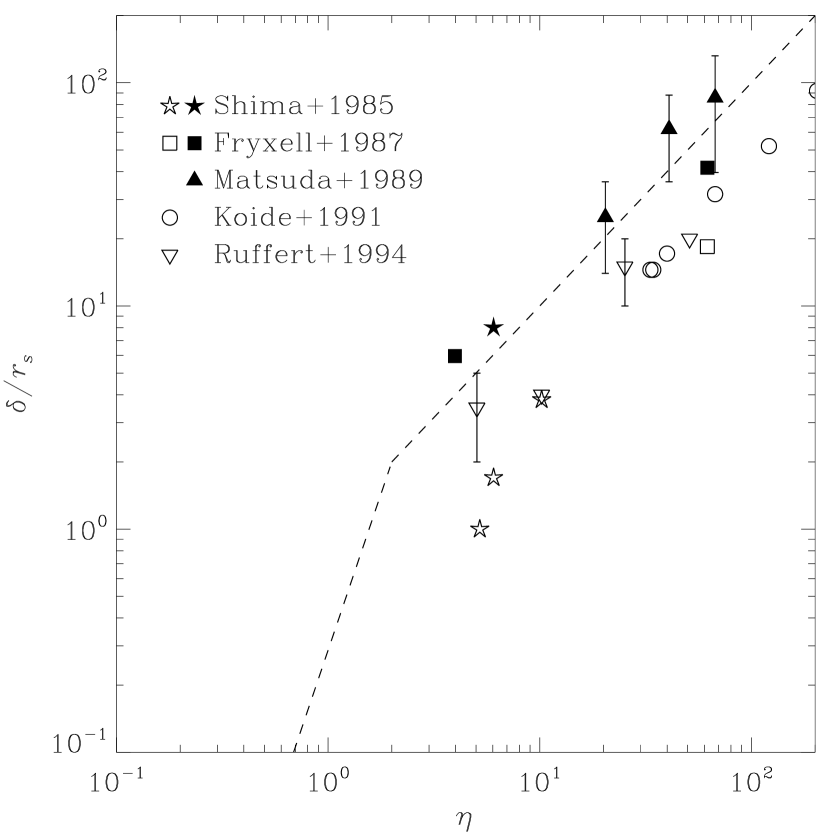
Figure 18: Detached shock distances against $\mathcal{\eta}$ from the published work on the BHL accretion flows. Open symbols denote the results when the matter is allowed to be absorbed to the perturber, while those under the reflection boundary conditions are given by filled symbols. For comparison, the broken power laws that fit our numerical results well are also shown as dashed lines.

Despite these differences, the detached distances of bow shocks and the resulting DF forces appear to be not so sensitive to the boundary conditions adopted. Figure 18 plots the detached shock distances inferred from the results of two-dimensional axisymmetric simulations (Shima et al., 1985; Fryxell et al., 1987; Matsuda et al., 1989; Koide et al., 1991) and the tabulated values from three-dimensional nonaxisymmetric runs (Ruffert, 1994) for the BHL accretion flows, by taking $r_{s}$ equal to the radius of the perturber. The BHL results under the reflecting boundary conditions are larger than our results by a factor of only $\sim 1.2$, while those under the absorbing boundary conditions are smaller by a factor of $\sim 0.4$. Since the work on the BHL accretion mostly focused on mass accretion rates, only a few of them evaluated the gravitational drag forces. In Figure 15, we plot using star symbols the drag forces from the adiabatic runs with $\gamma=5/3$ in Shima et al. (1985), which are the only data we acquired from the literature that allow a reliable comparison with our results. Note that the drag force is larger on a purely-absorbing perturber for which the detached shock distance is smaller. The DF forces from Shima et al. (1985) are roughly consistent with, and follow a similar trend to, our results. This is probably because even though density wakes are nowhere close to being hydrostatic in BHL accretion flows, they somehow maintain front-back symmetry that makes the net DF force smaller.

While we have considered in this paper only an adiabatic gas with index $\gamma=5/3$, we note that the DF force may depends sensitively on $\gamma$. Simulations of the BHL accretion flows reported that as $\gamma$ decreases, the detached shock distance decreases and the density wake becomes shaped increasingly into a cone-like structure similar to the linear wake (Hunt, 1979; Shima et al., 1985; Ruffert, 1995, 1996). This is presumably because bow shocks in lower-$\gamma$ models should be stronger in order to compensate for the diminished pressure in supporting the postshock gas against the perturber’s gravity. Consequently, drag forces are larger for the gas with smaller $\gamma$ (Shima et al., 1985).

Escala et al. (2005) carried out numerical simulations of a DF-induced merger of supermassive binary black holes due to an adiabatic gas with $\gamma=5/3$. Their Figure 9 presents the effect of the black hole mass on the evolution of the binary separation. From this figure, we infer that the orbital decay time scales with the black hole mass as $\tau_{\rm decay}\propto M_{p}^{-0.3}$ in their simulations, which is somewhat shallower than the linear expectation of $\tau_{\rm decay}\propto M_{p}^{-1}$ (e.g., Ostriker 1999). On the other hand, our results predict $\tau_{\rm decay}\propto M_{p}^{-0.55}$ if the perturber is sufficiently massive, suggesting that the delayed orbital decay of supermassive black holes in Escala et al. (2005) is partly due to the nonlinear effect. Of course, there are many other factors that may change $\tau_{\rm decay}$. While we consider quite an ideal situation in which a perturber is moving straight in a static, uniform medium, the gas in Escala et al. (2005) is distributed in a rotating, radially-stratified, self-gravitating disk and the black holes follow curvilinear, possibly eccentric, orbits. In addition, the Mach number of the black holes in their models is likely to vary during the decay toward the orbital center, which may also modify the decay time. Since these compact objects have a very small size, it is also an issue whether numerical models resolve detached bow shocks, which is crucial in evaluating the drag force accurately. We will discuss these in subsequent work.

Appendix A Linear Solution for the Velocity Wake

Using the Fourier transform for the space variables and the Laplace transform for the time variable, Just & Kegel (1990) derived an analytic solution for the velocity field in the linear wake, but unfortunately the resulting expression (their equation [47]) contains an typographical mistake. Here we rederive the expression using Fourier transforms for both space and time variables. We consider a point-mass perturber with mass $M_{p}$ on a straight-line trajectory through a uniform medium with density $\rho_{\infty}$ and adiabatic sound speed $a_{\rm\infty}$. The basic equations of hydrodynamics for an inviscid, nonmagnetic, non-self-gravitating gas are

$$\frac{\partial\rho}{\partial t}+\mbox{\boldmath{$\nabla$}}\cdot(\rho\mbox{\boldmath{$v$}})=0,$$ (A1)

and

$$\frac{\partial\mbox{\boldmath{$v$}}}{\partial t}+\mbox{\boldmath{$v$}}\cdot\mbox{\boldmath{$\nabla$}}\mbox{\boldmath{$v$}}=-\frac{1}{\rho}\mbox{\boldmath{$\nabla$}}P-\mbox{\boldmath{$\nabla$}}\Phi_{\rm ext},$$ (A2)

where $\Phi_{\rm ext}$ is the gravitational potential of the perturber with density $\rho_{\rm ext}$, satisfying the Poisson equation $\mbox{\boldmath{$\nabla$}}^{2}\Phi_{\rm ext}=4\pi G\rho_{\rm ext}$. Assuming that the density and velocity fields induced by the perturber have small amplitudes, we linearize equations (A1) and (A2) to obtain

$$\frac{\partial\alpha}{\partial t}+\mbox{\boldmath{$\nabla$}}\cdot\mbox{\boldmath{$v$}}=0,$$ (A3)

and

$$\frac{\partial\mbox{\boldmath{$v$}}}{\partial t}+a_{\rm\infty}^{2}\mbox{\boldmath{$\nabla$}}\alpha=-\mbox{\boldmath{$\nabla$}}\Phi_{\rm ext},$$ (A4)

where $\alpha\equiv\rho/\rho_{\infty}-1$ is the dimensionless perturbed density.

Taking Fourier transformation of equations (A3) and (A4), we have

$$\left(k^{2}-\frac{\omega^{2}}{a_{\rm\infty}^{2}}\right)\widehat{\alpha}=\frac{4\pi G}{a_{\rm\infty}^{2}}\widehat{\rho}_{\rm ext}$$ (A5)

and

$$\widehat{\mbox{\boldmath{$v$}}}=\frac{\omega\mbox{\boldmath{$k$}}}{k^{2}}\widehat{\alpha},$$ (A6)

where symbols with and without hat denote a Fourier pair defined by

$$\Psi(\mbox{\boldmath{$x$}},t)=\frac{1}{(2\pi)^{4}}\int\!\!\!\!\int\!\!\!\!\int\!\!\!\!\int\widehat{\Psi}(\mbox{\boldmath{$k$}},\omega)e^{i(\mbox{\boldmath{$k$}}\cdot\mbox{\boldmath{$x$}}-\omega t)}\,d^{3}\mbox{\boldmath{$k$}}\,d\omega$$ (A7)

and

$$\widehat{\Psi}(\mbox{\boldmath{$k$}},\omega)=\int\!\!\!\!\int\!\!\!\!\int\!\!\!\!\int\Psi(\mbox{\boldmath{$x$}},t)e^{-i(\mbox{\boldmath{$k$}}\cdot\mbox{\boldmath{$x$}}-\omega t)}\,d^{3}\mbox{\boldmath{$x$}}\,dt,$$ (A8)

with $\Psi$ representing any physical quantities.

For a perturber introduced at $t=0$ and moving at a constant speed $V_{p}$ along the positive $z$-direction, $\rho_{\rm ext}=M_{p}\,\delta(\mbox{\boldmath{$x$}}-V_{p}t\mbox{\boldmath{$\mathrm{e_{z}}$}})\,\mathcal{H}(t)$, where $\delta(\mbox{\boldmath{$x$}})$ is the Kronecker delta and $\mathcal{H}(t)$ is a Heaviside step function. This results in

$$\widehat{\rho}_{\rm ext}=M_{p}\left[2\pi\delta(\omega-k_{z}V_{p})+\frac{i}{\omega-k_{z}V_{p}}\right].$$ (A9)

The second term in equation (A9) is originated from the step function, which vanishes if a steady state is assumed (e.g., Furlanetto & Loeb, 2002).

Substituting equation (A9) into equation (A5), and taking an inverse Fourier transform of the resulting expression for $\widehat{\alpha}$, one can obtain the solution of the perturbed density for finite-time perturbations. The detailed procedure is similar to that of the Fourier-Laplace transform method of Just & Kegel (1990), so that we simply write the result

$$\alpha=\frac{GM_{p}}{a_{\rm\infty}^{2}}\frac{\Upsilon_{1}}{(s^{2}+R^{2}(1-\mathcal{M}^{2}))^{1/2}},$$ (A10)

where $s\equiv z-V_{p}t$ and $\Upsilon_{1}=2$, 1, and 0 in region I ($R^{2}+z^{2}>a_{\rm\infty}^{2}t^{2},\ R^{2}<-sz,\ s^{2}+R^{2}(1-\mathcal{M}^{2})>0$, $\mathcal{M}>1$), region II ($R^{2}+z^{2}<a_{\rm\infty}^{2}t^{2}$), and any other region, respectively. Note that equation (A10) is identical to equation (10) of Ostriker (1999) based on the retarded Green’s function technique.

Combining equations (A5), (A6), and (A9) together in favor of $\widehat{\mbox{\boldmath{$v$}}}$ and taking its inverse Fourier transform, we have

$$\mbox{\boldmath{$v$}}=\frac{GM_{p}}{4\pi^{3}a_{\rm\infty}^{2}}\int\!\!\!\!\int\!\!\!\!\int\!\!\!\!\int\bigg{[}\frac{2\pi\delta(\omega-k_{z}V_{p})}{k^{2}-\omega^{2}/a_{\rm\infty}^{2}}+\frac{i}{(k^{2}-\omega^{2}/a_{\rm\infty}^{2})(\omega-k_{z}V_{p})}\bigg{]}\frac{\omega\mbox{\boldmath{$k$}}}{k^{2}}e^{i(\mbox{\boldmath{$k$}}\cdot\mbox{\boldmath{$x$}}-\omega t)}\,d^{3}\mbox{\boldmath{$k$}}\,d\omega.$$ (A11)

The second term in the integrand of equation (A11) has three simple poles on the real $\omega$ axis at $\omega_{1}=k_{z}V_{p}$ and $\omega_{2,3}=\pm ka_{\rm\infty}$. To ensure the proper analyticity, we must displace them by an infinitesimal amount into the upper or lower half $\omega$-plane. Since our problem requires $\mbox{\boldmath{$v$}}=0$ everywhere for $t<0$, the proper choice of the pole displacements should be $\omega_{1}$ into the upper half $\omega$-plane and $\omega_{2,3}$ to the lower half $\omega$-plane. For $t<0$, then, a contour of integration consisting of the real $\omega$ axis and an infinitely-large semicircle in the upper half $\omega$-plane encloses only $\omega_{1}$, and the calculus of residues guarantees that after the integration over $\omega$, the first and second terms in the integrand of equation (A11) become identical with each other with opposite sign, resulting in no velocity perturbations before the introduction of the perturber.

For $t>0$, the contour that goes along an infinitely-large semicircle in the lower half $\omega$-plane instead contains the poles at $\omega_{2,3}$. The remaining steps in the integration with respect to $\omega$ is quite straightforward to yield

$$\mbox{\boldmath{$v$}}=\frac{GM_{p}}{4\pi^{2}a_{\rm\infty}}\int\!\!\!\!\int\!\!\!\!\int\bigg{(}\frac{e^{ika_{\rm\infty}t}-e^{-ik_{z}V_{p}t}}{k+k_{z}\mathcal{M}}-\frac{e^{-ika_{\rm\infty}t}-e^{-ik_{z}V_{p}t}}{k-k_{z}\mathcal{M}}\bigg{)}\frac{\mbox{\boldmath{$k$}}}{k^{2}}e^{i\mbox{\boldmath{$k$}}\cdot\mbox{\boldmath{$x$}}}\,d^{3}\mbox{\boldmath{$k$}}.$$ (A12)

To carry out the integration in equation (A12), it is convenient to use spherical coordinates in the $k$-space as

$$\mbox{\boldmath{$k$}}=k\,(\sin\theta\cos(\varphi+\zeta),\sin\theta\sin(\varphi+\zeta),\cos\theta),$$ (A13)

which is oriented relative to the space coordinates

$$\mbox{\boldmath{$x$}}=(R\cos\zeta,R\sin\zeta,z),$$ (A14)

satisfying $\mbox{\boldmath{$k$}}\cdot\mbox{\boldmath{$x$}}=k\,(z\cos\theta+R\sin\theta\cos\varphi)$. We then obtain

$$\mbox{\boldmath{$v$}}=\frac{GM_{p}}{4\pi^{2}a_{\rm\infty}}\int\!\!\!\!\int\!\!\!\!\int\bigg{[}\frac{e^{ik(z\cos\theta+a_{\rm\infty}t)}-e^{iks\cos\theta}}{1+\mathcal{M}\cos\theta}-\frac{e^{ik(z\cos\theta-a_{\rm\infty}t)}-e^{iks\cos\theta}}{1-\mathcal{M}\cos\theta}\bigg{]}e^{ikR\sin\theta\cos\varphi}$$

$$\times(\sin^{2}\theta\cos(\varphi+\zeta)\mbox{\boldmath{$\mathrm{e_{x}}$}}+\sin^{2}\theta\sin(\varphi+\zeta)\mbox{\boldmath{$\mathrm{e_{y}}$}}+\sin\theta\cos\theta\mbox{\boldmath{$\mathrm{e_{z}}$}})\,\,dk\,d\theta\,d\varphi,$$ (A15)

where $\mathrm{e_{x}}$, $\mathrm{e_{y}}$, and $\mathrm{e_{z}}$ are the unit vectors in the $x$-, $y$-, and $z$-directions, respectively. Without loss of generality, we take $\zeta=0$, in which case $\mathrm{e_{x}}$ and $\mathrm{e_{y}}$ correspond to the unit vectors in the radial ($\mathrm{e_{R}}$) and azimuthal ($\mathrm{e_{\varphi}}$) directions, respectively. It then follows that the azimuthal velocity vanishes (i.e., $v_{\varphi}=0$) since this component in the integrand is an odd function of $\varphi$.

For the velocity component in the direction of motion, we substitute $\theta=\pi-\theta^{\prime}$ to the second term inside the square bracket of equation (A) to obtain

$$v_{z}=\frac{GM_{p}}{\pi a_{\rm\infty}}\int^{\pi}_{0}\!\!\!d\theta\!\int^{\infty}_{0}\!\!\!dk\,\frac{\sin\theta\cos\theta J_{0}(kR\sin\theta)}{1+\mathcal{M}\cos\theta}\left\{\cos[k(z\cos\theta+a_{\rm\infty}t)]-\cos(ks\cos\theta)\right\}.$$ (A16)

Using [G6.671.8], inserting the substitutions

$$\sin\eta=\frac{(R^{2}+z^{2})\cos\theta+za_{\rm\infty}t}{R(R^{2}+z^{2}-a_{\rm\infty}^{2}t^{2})^{1/2}}$$ (A17)

and

$$\sin\eta=\frac{(R^{2}+s^{2})^{1/2}}{R}\cos\theta,$$ (A18)

for the first and second terms of equation (A16), respectively, and applying [G2.551.3] for the $\eta$-integrations, we obtain

$$v_{z}=-\frac{GM_{p}}{V_{p}}\left[\frac{1}{(R^{2}+s^{2})^{1/2}}-\frac{\Upsilon_{1}}{(s^{2}+R^{2}(1-\mathcal{M}^{2}))^{1/2}}-\frac{\Upsilon_{2}}{(R^{2}+z^{2})^{1/2}}\right],$$ (A19)

where $\Upsilon_{1}=$2, 1, 0 and $\Upsilon_{2}=1$, 0, 1 for region I ($R^{2}+z^{2}>a_{\rm\infty}^{2}t^{2},\ R^{2}<-sz,\ s^{2}+R^{2}(1-\mathcal{M}^{2})>0$, $\mathcal{M}>1$), region II ($R^{2}+z^{2}<a_{\rm\infty}^{2}t^{2}$), and any other region, respectively.

For the velocity component in the radial direction, the use of [G6.671.1] similarly leads to

$$v_{R}=\frac{GM_{p}}{RV_{p}}\left[\frac{s}{(R^{2}+s^{2})^{1/2}}-\frac{s\Upsilon_{1}}{(s^{2}+R^{2}(1-\mathcal{M}^{2}))^{1/2}}-\frac{z\Upsilon_{2}}{(R^{2}+z^{2})^{1/2}}\right].$$ (A20)

The results of our time-dependent linear analyses for density and velocity fields are confirmed by direct numerical simulations for a low-mass perturber with $\mathcal{A}=0.01$ presented in §3.

In terms of our notation, equation (47) of Just & Kegel (1990) can be rewritten as

$$(v_{R},v_{z})=\frac{GM_{p}}{RV_{p}}\left[\frac{(s,-R)}{(R^{2}+s^{2})^{1/2}}-\frac{(s,-R)\Upsilon_{1}}{(s^{2}+R^{2}(1-\mathcal{M}^{2}))^{1/2}}-\frac{(z,-R)}{(R^{2}+z^{2})^{1/2}}\right].$$ (A21)

Comparison of equation (A21) with equations (A19) and (A20) shows that equation (47) of Just & Kegel (1990) takes $\Upsilon_{2}=1$ everywhere, which is clearly incorrect.

Figure 2: Distributions of the perturbed density along the cuts at $R/a_{\rm\infty}t=0.20$ (top) and $z/a_{\rm\infty}t=0.92$ (bottom) indicated as dotted lines in Fig. 1 of a model with $\mathcal{A}=0.01$ and $\mathcal{M}=1.5$. Open circles representing the simulation results deviate considerably from the results $\alpha$ (dashed line) of the linear perturbation theory for a point mass, but are in excellent agreement with $\alpha_{\rm ext}$ (solid line) obtained from the convolution of $\alpha$ with the extended mass distribution.

Figure 3: Dimensionless DF force on a low-mass perturber with $\mathcal{A}=0.01$ against the Mach number $\mathcal{M}$ at $t/t_{\rm cross}=300$. The solid line is the best fit of the linear force formula (eq. [1]) with $r_{\rm min}=0.35\mathcal{M}^{0.6}r_{s}$ to our simulation results (open squares).

Figure 5: Time evolution of the detached shock distance $\delta$ measured along the symmetry axis from the perturber center for various models. For each model with $\mathcal{A}\leq 50$, $\delta$ initially increases rapidly with time, experiences quasi-periodic oscillations, and then saturates to a constant value. The time to reach a quasi-steady state and the value of $\delta$ at saturation become smaller as $\mathcal{A}$ decreases or $\mathcal{M}$ increases; the model with $\mathcal{A}=100$ and $\mathcal{M}=1.5$ does not attain a quasi-steady state until the end of run.

Figure 6: Trajectory of the center of the primary vortex on the $s$–$R$ plane for a model with $A=20$ and $\mathcal{M}=1.5$. Filled circles marked by alphabets a–h indicate the vortex locations at time epochs corresponding to the snapshots shown in Fig. 4. The dotted curve draws the region where the distance from the perturber equals a half of accretion radius $r_{\rm A}\equiv 2GM_{p}/V_{p}^{2}$.

Figure 9: Density profiles along the positive-$z$ (solid), negative-$z$ (dashed), and $R$ (dot-dashed) axes from the perturber center for (a) a supersonic model with $\mathcal{A}=20$ and $\mathcal{M}=1.5$ and (b) a subsonic model with $\mathcal{A}=20$ and $\mathcal{M}=0.5$ at $t/t_{\rm cross}=600$. In each panel, the dotted line gives the respective density distribution under the assumption of hydrostatic equilibrium, which is in good agreement with the numerical results for $r/r_{s}\lesssim 10$.

Figure 10: Distributions of normalized perturbed density $\alpha/\mathcal{A}$ as functions of $s$ along the (a) $R=0$ and (b) $R/r_{s}=200$ cuts for models shown in Figure 8. While $\alpha/\mathcal{A}$ near the perturber with $\mathcal{A}\geq 1$ deviates significantly from that of the linear case, it becomes nearly independent of $\mathcal{A}$ in the regions far away from the perturber. For $\mathcal{A}\geq 1$, $\alpha$ shows some fluctuations and becomes negative in some regions near the symmetry axis ($R=0$) behind the perturber, since the flow in these regions already experienced strong perturbations in the upstream region.

Figure 11: Detached shock distance $\delta$ as a function of the nonlinearity parameter $\mathcal{\eta}=\mathcal{A}/(\mathcal{M}^{2}-1)$. Various symbols and errorbars give the means and standard deviations of $\delta$ over time for $t/t_{\rm cross}>50$. Dashed lines correspond to the broken power laws $\delta/r_{s}=2(\eta/2)^{2.8}$ for $0.7\lesssim\eta\lesssim 2$ and $\delta/r_{s}=\eta$ for $\eta\gtrsim 2$ that describe the numerical data quite well.

Figure 12: Dimensionless detached shock distance as a function of the Mach number. Various symbols and errorbars give the means and standard deviations of $\delta/r_{\rm BHL}$ over time for $t/t_{\rm cross}>50$, where $r_{\rm BHL}$ is the BHL radius. The solid curve plots equation (9) for $\delta/R_{s}$, the ratio of the standoff distance of the shock to the radius of a spherical body in the non-gravitating hydrodynamic theory.

Figure 13: Temporal changes of the dimensionless DF forces for models with $\mathcal{M}=1.5$. The dotted line is the prediction of equation (1) with $r_{\rm min}=0.35\mathcal{M}^{0.6}r_{s}$, in good agreement with the numerical result for a low-mass perturber with $\mathcal{A}=0.01$. The drag forces increase logarithmically with time, although models with large $\mathcal{A}$ exhibit early fluctuations in accordance with shock oscillations.

Figure 14: Dimensionless DF forces for various models with different $\mathcal{A}$ and $\mathcal{M}$ at $t/t_{\rm cross}=600$. The solid line draws the linear drag force (eq. [1]) with $r_{\rm min}=0.35\mathcal{M}^{0.6}r_{s}$. For supersonic models, the drag force decreases with increasing $\mathcal{A}$. Subsonic models do not reach a quasi-steady state and show some fluctuations, but their mean drag forces are similar to the linear estimates with the same $\mathcal{M}$.

Figure 15: Ratio of the nonlinear to linear DF forces for supersonic models as a function of the nonlinearity parameter $\mathcal{\eta}=\mathcal{A}/(\mathcal{M}^{2}-1)$. Various symbols and their errorbars indicate the means and standard deviations of $F/F_{\rm lin}$ over time for $t/t_{\rm cross}>50$. When $\mathcal{\eta}\lesssim 0.7$, $F/F_{\rm lin}\approx 1$, while $F/F_{\rm lin}\approx(\eta/2)^{-0.45}$ for $\mathcal{\eta}>2$. Also plotted as star symbols are the results of Shima et al. (1985) for BHL flows onto accreting or reflecting bodies.

Figure 16: Dimensionless DF force as a function of the cut-off radius $r_{\rm min}$, interior of which is excluded in the force evaluation, for a model with $\mathcal{A}=20$ and $\mathcal{M}=1.5$ at $t/t_{\rm cross}=600$. The vertical dashed line marks the detached shock distance of $\delta=12r_{s}$, while the dotted line indicates a slope of $-1$. The drag force is nearly constant for $r_{\rm min}\lesssim\delta$ and decreases almost logarithmically at large $r_{\rm min}$.

Figure 17: Time evolution of (a) the detached shock distance $\delta$ and (b) the dimensionless DF force $F$ for $\mathcal{A}=10$ and $\mathcal{M}=1.5$. The simulation results at four different resolutions are compared. Note that $\delta$ and $F$ are fully resolved if $\Delta z/r_{s}\gtrsim 0.2$, where $\Delta z$ is the grid spacing.

References

- Alibert et al. (2005) Alibert, Y., Mordasini, C., Benz, W., & Winisdoerffer, C. 2005, A&A, 434, 343
- Armitage & Rice (2005) Armitage, P. J., & Rice, W. K. M. 2005, astro-ph/0507492
- Barausse (2007) Barausse, E. 2007, MNRAS, 382, 826
- Bondi & Hoyle (1944) Bondi, H., & Hoyle, F. 1944, MNRAS, 104, 273
- Bondi (1952) Bondi, H. 1952, MNRAS, 112, 195
- Butler et al. (2006) Butler, R. P., Wright, J. T., Marcy, G. W. et al. 2006, ApJ, 646, 505
- Chandrasekhar (1943) Chandrasekhar, S. 1943, ApJ, 97, 255
- Colella & Woodward (1984) Colella, P., & Woodward, P. R. 1984, Journal of Computational Physics, 54, 174
- Conroy & Ostriker (2008) Conroy, C., & Ostriker, J. P. 2008, ApJ, 681, 151
- Cuadra et al. (2009) Cuadra, J., Armitage, P. J., Alexander, R. D., & Begelman, M. C. 2009, MNRAS, 393, 1423
- Dokuchaev (1964) Dokuchaev, V. P. 1964, Soviet Astron., 8, 23
- Dotti et al. (2006) Dotti, M., Colpi, M., & Haardt, F. 2006, MNRAS, 367, 103
- Dotti et al. (2007) Dotti, M., Colpi, M., Haardt, F., & Mayer, L. 2007, MNRAS, 379, 956
- Edgar (2004) Edgar, R. 2004, New Astronomy Reviews, 48, 843
- El-Zant et al. (2004) El-Zant, A. A., Kim, W.-T., & Kamionkowski, M. 2004, MNRAS, 354, 169
- Escala et al. (2004) Escala, A., Larson, R. B., Coppi, P. S., & Mardones, D. 2004, ApJ, 607, 765
- Escala et al. (2005) Escala, A., Larson, R. B., Coppi, P. S., & Mardones, D. 2005, ApJ, 630, 152
- Faltenbacher et al. (2005) Faltenbacher, A., Kravtsov, A. V., Nagai, D., & Gottloeber, S. 2005, MNRAS, 358, 139
- Foglizzo & Ruffert (1997) Foglizzo, T., & Ruffert, M. 1997, A&A, 320, 342
- Foglizzo & Ruffert (1999) Foglizzo, T., & Ruffert, M. 1999, A&A, 347, 901
- Foglizzo et al. (2005) Foglizzo, T., Galletti, P., & Ruffert, M. 2005, A&A, 435, 397
- Fryxell et al. (1987) Fryxell, B. A., Taam, R. E., & McMillan, S. L. W. 1987, ApJ, 315, 536
- Fryxell & Taam (1988) Fryxell, B. A., & Taam, R. E., 1988, ApJ, 335, 862
- Fryxell et al. (2000) Fryxell, B,. Olson, K., Ricker, P., Timmes, F. X., Zingale, M., Lamb, D. Q., MacNeice, P., Rosner, R., Truran, J. W., & Tufo, H. 2000, ApJS, 131, 273
- Furlanetto & Loeb (2002) Furlanetto, S. R., & Loeb, A. 2002, ApJ, 565, 854
- Gradshteyn & Ryzhik (1994) Gradshteyn, I. S., & Ryzhik, I. M. 1994, Table of Integrals, Series, and Products (New York: Academic Press)
- Guy (1974) Guy, T. B. 1974, AIAA Journal, 12, 380
- Heberle et al. (1950) Heberle, J. W., Wood, G. P., & Gooderum, P. B. 1950, NASA TN 2000
- Hoyle & Lyttleton (1939) Hoyle, F., & Lyttleton, R. A. 1939, Proceedings of the Cambridge Philosophical Society, 34, 405
- Hunt (1971) Hunt, R. 1971, MNRAS, 154, 141
- Hunt (1979) Hunt, R. 1979, MNRAS, 188, 83
- Just & Kegel (1990) Just, A., & Kegel, W. H. 1990, A&A, 232, 447
- Karas & Šubr (2001) Karas, V., Šubr, L. 2001, A&A, 376, 686
- Kim & Kim (2007) Kim, H., & Kim, W.-T. 2007, ApJ, 665, 432
- Kim et al. (2008) Kim, H., Kim, W.-T., & Sánchez-Salcedo, F. J. 2008, ApJ, 679, L33
- Kim et al. (2005) Kim, W.-T., El-Zant, A. A., & Kamionkowski, M. 2005, ApJ, 632, 157
- Kim (2007) Kim, W.-T. 2007, ApJ, 667, L5
- Koide et al. (1991) Koide, H., Matsuda, T., & Shima, E. 1991, MNRAS, 252, 473
- Liepmann & Roshko (1957) Liepmann, H., & Roshko, A. 1957, Elements of Gasdynamics, Galcit Aeronautical Series (New York: Wiley, 1957)
- Matsuda et al. (1987) Matsuda, T., Inoue, M., & Sawada, K. 1987, MNRAS, 226, 785
- Matsuda et al. (1989) Matsuda, T., Sekino, N., Shima, E., & Sawada, K. 1989, MNRAS, 236, 817
- Mayer et al. (2007) Mayer, L., Kazantzidis, S., Madau, P., Colpi, M., Quinn, T., & Wadsley, J. 2007, Science, 316, 1874
- Milosavljević & Merritt (2003) Milosavljević, M., & Merritt, D. 2003, in AIP Conf. Proc. 686, The Astrophysics of Gravitational Wave Sources, ed. J. M. Centrella (New York: AIP), 201
- Narayan (2000) Narayan, R. 2000, ApJ, 536, 663
- Ostriker (1999) Ostriker, E. C. 1999, ApJ, 513, 252
- Rephaeli & Salpeter (1980) Rephaeli, Y., & Salpeter, E. E. 1980, ApJ, 240, 20
- Ruderman & Spiegel (1971) Ruderman, M. A., & Spiegel, E. A. 1971, ApJ, 165, 1
- Ruffert (1994) Ruffert, M. 1994, A&AS, 106, 505
- Ruffert (1995) Ruffert, M. 1995, A&AS, 113, 133
- Ruffert (1996) Ruffert, M. 1996, A&A, 311, 817
- Ruffert (1999) Ruffert, M. 1999, A&A, 346, 861
- Sánchez-Salcedo & Brandenburg (1999) Sánchez-Salcedo, F. J., & Brandenburg, A. 1999, ApJ, 522, L35
- Sánchez-Salcedo & Brandenburg (2001) Sánchez-Salcedo, F. J., & Brandenburg, A. 2001, MNRAS, 322, 67
- Schreier (1982) Schreier, S. Compressible Flow (John Wiley & Sons), 185
- Schwartz & Eckerman (1956) Schwartz, R. N., & Eckerman, J. 1956, Journal of Applied Physics, 27, 169
- Shankar et al. (1993) Shankar, A., Kley, W., & Burkert, A. 1993, A&A, 274, 955
- Shima et al. (1985) Shima, E., Matsuda, T., Takeda, H., & Sawada, K. 1985, MNRAS, 217, 367
- Taam & Fryxell (1988) Taam, R. E., & Fryxell, B. A. 1988, ApJ, 327, L73
- van Dyke & Milton (1958) van Dyke, M. D., & Milton, D. 1958, Journal of the Aeronautical Sciences, 25, 485