A Stochastic Phase-Field Model
Computed From Coarse-Grained Molecular Dynamics

Abstract

Results are presented from numerical experiments aiming at the computation of stochastic phase-field models for phase transformations by coarse-graining molecular dynamics. The studied phase transformations occur between a solid crystal and a liquid. Nucleation and growth, sometimes dendritic, of crystal grains in a sub-cooled liquid is determined by diffusion and convection of heat, on the macroscopic level, and by interface effects, where the width of the solid–liquid interface is on an atomic length-scale. Phase-field methods are widely used in the study of the continuum level time evolution of the phase transformations; they introduce an order parameter to distinguish between the phases. The dynamics of the order parameter is modelled by an Allen–Cahn equation and coupled to an energy equation, where the latent heat at the phase transition enters as a source term. Stochastic fluctuations are sometimes added in the coupled system of partial differential equations to introduce nucleation and to get qualitatively correct behaviour of dendritic side-branching. In this report the possibility of computing some of the Allen–Cahn model functions from a microscale model is investigated. The microscopic model description of the material by stochastic, Smoluchowski, dynamics is considered given. A local average of contributions to the potential energy in the micro model is used to determine the local phase, and a stochastic phase-field model is computed by coarse-graining the molecular dynamics. Molecular dynamics simulations on a two phase system at the melting point are used to compute a double-well reaction term in the Allen–Cahn equation and a diffusion matrix describing the noise in the coarse-grained phase-field.

This work was supported by the Swedish Foundation for Strategic Research grant A3 02:123, ”Mathematical theory and simulation tools for phase transformations is materials”.

1 Introduction

Phase-field methods are widely used for modelling phase transformations in materials on the continuum level and exist in many different versions for different applications. In this report the considered phase transformation occurs in a single component system with a solid and a liquid phase.

The phase-field model of solidification studied here is a coupled system of partial differential equations for the temperature, $T$, and a phase-field, $\phi$, which is an order parameter used to distinguish between the solid and the liquid subdomains. Two different values, ${\phi}_{s}$ and ${\phi}_{l}$, are equilibrium values of the phase-field in solid and liquid respectively. The phase-field varies continuously between the two values and the interface between solid and liquid, at a time $t$, is defined as a level surface of the phase-field; for example $\{x\in\mathbb{R}^{d}\,\colon\,{\phi}(x,t)=0.5({\phi}_{s}+{\phi}_{l})\}$. From a computational point of view the implicit definition of the phases in the phase-field method, as in the level set method [8, 12], is an advantage over sharp interface methods, since it avoids the explicit tracking of the interface. A local change of the phase-field from ${\phi}_{l}$ to ${\phi}_{s}$ in a subdomain translates into solidification of that region with a corresponding release of latent heat and the reverse change from ${\phi}_{s}$ to ${\phi}_{l}$ means melting which requires energy. The release or absorption of latent heat is modelled as a continuous function of $\phi$ so that the energy released when a unit volume solidifies is ${L}({g}({\phi}_{l})-{g}({\phi}_{s}))$, where $L$ is the latent heat and ${g}({\phi})$ is a model function, monotone with ${g}({\phi}_{s})=0$, ${g}({\phi}_{l})=1$, ${g}^{\prime}({\phi}_{s})=0$, and ${g}^{\prime}({\phi}_{l})=0$. Then the energy equation for a unit volume becomes a heat equation with a source term

$$\frac{\partial}{\partial t}\left({c_{V}}{T}+{L}{g}({\phi})\right) =\nabla\cdot\left({\lambda}\nabla{T}\right),$$

where $c_{V}$ is the heat capacity at constant volume and $\lambda$ is the thermal conductivity. Here, and in the following, the usual notation for differentiation with respect to the spatial variables is applied, with $\nabla$ and $\nabla\cdot$ denoting the gradient and the divergence respectively. The phase-field, and the related model function $g$, are exceptional in the energy equation in the sense that, while all the other quantities are standard physical quantities on the macroscopic level, the phase-field need not be associated with a measurable quantity. A phenomenological model of the phase change is given by the energy equation coupled to the Allen-Cahn equation

$$\frac{\partial{\phi}}{\partial t} =\nabla\cdot\left(k_{1}\nabla{\phi}\right)-k_{2}\Big{(}{f}^{\prime}({\phi})+{g}^{\prime}({\phi})k_{3}({T_{\mathrm{M}}}-{T})\Big{)}$$ (1)

for the time evolution of the phase-field; here $T_{\mathrm{M}}$ denotes the melting point, $k_{1}$, $k_{2}$, and $k_{3}$, are positive model parameters ($k_{1}$ may be an anisotropic matrix introducing directional dependence on the growth of the solid), and the model function $f$ is a double well potential with minima at ${\phi}_{s}$ and ${\phi}_{l}$. Standard examples of the model functions are

$${f}({\phi}) =-\frac{1}{2}{\phi}^{2}+\frac{1}{4}{\phi}^{4}, {g}({\phi}) =\frac{15}{16}\left(\frac{1}{5}{\phi}^{5}-\frac{2}{3}{\phi}^{3}+{\phi}\right)+\frac{1}{2},$$

when ${\phi}_{s}=-1$ and ${\phi}_{l}=1$. By construction of the model functions, the reaction term in the Allen-Cahn equation vanishes where ${\phi}={\phi}_{s}$ or ${\phi}={\phi}_{l}$ independently of the temperature. Since the diffusion term is zero for any constant function the two constant phase-fields ${\phi}\equiv{\phi}_{s}$ and ${\phi}\equiv{\phi}_{l}$ are stationary solutions to the Allen-Cahn equation for all temperatures. This means, for example, that nucleation of solid in a region of subcooled liquid can not occur in a phase-field modelled by the deterministic Allen-Cahn equation above. The effect of nucleation can be introduced in the model by adding a noise term in the Allen-Cahn equation, giving a stochastic partial differential equation. Simulation of dendrite growth in an subcooled liquid is another example where the deterministic system is inadequate; its solutions fail to develop the side branches seen to form in real dendrites as the tips grow. Stochastic phase-field models where noise is added to either one, or both, of the Allen-Cahn equation and the energy equation are used to include the effect of side branching; see for example [2].

The present report contains the results from numerical experiments on a method presented and analysed in [14] and the rest of this introduction summarises the ideas from [14] needed here. That report takes the stochastic phase-field model

$$\frac{\partial}{\partial t}\left({c_{V}}{T}+{L}{g}({\phi})\right) =\nabla\cdot\left({\lambda}\nabla{T}\right),$$ (2a)

$$\frac{\partial{\phi}}{\partial t} =\nabla\cdot\left(k_{1}\nabla{\phi}\right)-k_{2}\Big{(}{f}^{\prime}({\phi})+{g}^{\prime}({\phi})k_{3}({T_{\mathrm{M}}}-{T})\Big{)}+\text{noise},$$ (2b)

as its starting point and asks whether it is possible to obtain the model functions and parameters, ${f}({\phi})$, ${g}({\phi})$, $k_{1}$, $k_{2}$, $k_{3}$, and the noise, from computations on a microscale model. To answer this question the phase-field, ${\phi}$, must be defined in terms of quantities computable on the microscale. The microscopic model used for this purpose is a molecular dynamics model of $N$ particles in a microscopic domain $D$ in $\mathbb{R}^{3}$ where the motion of the particles is given by the Smoluchowski dynamics; see for example [5]. Thus, with ${X_{{\mbox{}}}^{t}}\in\mathbb{R}^{3N}$ denoting the positions of all particles in the system at the time $t$ and ${X_{i}^{t}}\in\mathbb{R}^{3}$ the position of particle $i$, the dynamics are given by the Itô stochastic differential equations

$$d{X_{i}^{t}}=-\nabla_{{X_{i}^{{\mbox{}}}}}{U}({X_{{\mbox{}}}^{t}})\;dt+\sqrt{2{k_{\mathrm{B}}}{T}}\;dW_{i}^{t}, i=1,2,\ldots,{N},$$ (3)

where $U$ is the total potential energy of the system, $\nabla_{{X_{i}^{{\mbox{}}}}}$ denotes the gradient with respect to the position of particle $i$, $k_{\mathrm{B}}$ is the Boltzmann constant, and $W_{i}={(W_{i,1},W_{i,2},W_{i,3})^{\mathrm{T}}}$ are independent three dimensional Brownian motions, with independent components. The macroscopic temperature, $T$, is a constant input parameter in the microscopic model. We may identify the latent heat, in the macroscopic model, with the difference in total potential energy per unit volume of the liquid and the solid at the melting point, in the microscopic model. The idea is then to let the local contributions to the total potential energy define the phase variable. Since the potential energy decreases with the temperature even in a single phase system the equilibrium values of such a phase-field, $m$, unlike those of $\phi$, depend on the temperature; see Figure 1.

Figure 1: Schematic picture of ${m}({T})$ for a pure liquid (top curve) and a pure solid (bottom curve) and the latent heat as the jump in $m$ at a phase transition.

Assuming that in pure solid or pure liquid the phase-field, $m$, varies slowly, compared to the latent heat release, with the temperature close to the melting point, the energy equation becomes

$$\frac{\partial}{\partial t}\left({c_{V}}{T}+{m}\right) =\nabla\cdot\left({\lambda}\nabla{T}\right),$$

where $c_{V}$ and $\lambda$ are approximately the same as in (2a) for ${T}\approx{T_{\mathrm{M}}}$.

For a model where the total potential energy of the system can be naturally split into a sum of contributions arising from the interaction of individual atoms with their environment,

$${U}({{X_{{\mbox{}}}^{{\mbox{}}}}}) ={\sum_{i=1}^{N}}{m_{i}}({{X_{{\mbox{}}}^{{\mbox{}}}}}),$$ (4)

phase-fields can be introduced on the micro level by localised averages of these contributions; a given configuration ${X_{{\mbox{}}}^{{\mbox{}}}}$ defines a phase-field ${m}(\,\cdot\,;{{X_{{\mbox{}}}^{{\mbox{}}}}})\;\colon\;D\rightarrow\mathbb{R}$ through

$${m}(x;{{X_{{\mbox{}}}^{{\mbox{}}}}}) ={\sum_{i=1}^{N}}{m_{i}}({{X_{{\mbox{}}}^{{\mbox{}}}}}){\eta}(x-{X_{i}^{{\mbox{}}}}),$$ (5)

where the choice of mollifier, $\eta$, determines the spatial smoothness of the phase-field. If, for example, the potential energy is defined entirely by pairwise interactions

$${U}({{X_{{\mbox{}}}^{{\mbox{}}}}}) =\frac{1}{2}{\sum_{i=1}^{N}}{\sum_{k\neq i,k=1}^{N}}{\Phi}({X_{i}^{{\mbox{}}}}-{X_{k}^{{\mbox{}}}}),$$

as is common in simple molecular dynamics models, it is natural to let

$${m_{i}}({{X_{{\mbox{}}}^{{\mbox{}}}}}) =\frac{1}{2}{\sum_{k\neq i,k=1}^{N}}{\Phi}({X_{i}^{{\mbox{}}}}-{X_{k}^{{\mbox{}}}})$$

be particle $i$’s contribution to the total potential energy.

With the definition (5) of the potential energy phase-field, $m$, and with the microscopic system defined by (3) and (4), Itô’s formula gives a stochastic differential equation

$$d{m}(x;{X_{{\mbox{}}}^{t}}) ={\alpha}(x;{X_{{\mbox{}}}^{t}})\;dt+{\sum_{j=1}^{N}}\sum_{k=1}^{3}{\beta}_{j,k}(x;{X_{{\mbox{}}}^{t}})\;dW_{j,k}^{t},$$ (6)

for $m$ evaluated in a point $x\in D$. The drift, ${\alpha}(x;\cdot)$, and the diffusions, ${\beta}_{j,k}(x;\cdot)$, are explicitly known functions expressed in terms of the ${m}_{i}$:s, the mollifier, $\eta$, and their derivatives up to second order. While $m$ by definition is a continuous field it is still an atomic scale quantity since it is defined in terms the particle positions $X_{{\mbox{}}}^{t}$. A macroscopic phase-field, similar to $\phi$ in (2), must lose both the dependence on the particle positions, $X_{{\mbox{}}}^{t}$, and the explicit dependence on the microscale space variable $x$. To achieve this, a coarse-grained approximation ${m_{\mathrm{cg}}}(x)$ of ${m}(x)$ is introduced as a solution of a stochastic differential equation

$$d{m_{\mathrm{cg}}^{t}}(x) ={a}({m_{\mathrm{cg}}^{t}})(x)\;dt+{\sum_{j=1}^{M}}{b}_{j}({m_{\mathrm{cg}}^{t}})(x)\;d{\widetilde{W}}_{j}^{t},$$ (7)

where the independent Wiener processes ${\widetilde{W}}_{j}^{t}$, $j=1,2,\ldots,{M}\ll{N}$, also are independent of the Wiener processes $W_{i}$ in the micro model. Here the drift and diffusion coefficient functions, ${a}({m_{\mathrm{cg}}^{t}})$ and ${b}_{j}({m_{\mathrm{cg}}^{t}})$, may depend on more information about the coarse-grained phase-field than just the point value; compare the stochastic Allen-Cahn equation (2b), where the diffusion term in the drift contains second derivatives of the phase-field.

The choice of the coarse-grained drift and diffusion functions proceeds in two steps: first, finding a general form the coarse-grained equation where the drift and diffusion coefficient functions, defined as time averaged expected values of the microscopic drift and diffusions over simulation paths, still depend on the micro scale space variable, $x$; second, expressing the $x$ dependent coarse-grained drift and diffusion coefficients by drift and diffusion functions depending only on the phase-field $m_{\mathrm{cg}}$, using that $m_{\mathrm{cg}}$ is a smooth monotone function of $x$ in the interface.

In the first step, a coarse-grained stochastic differential equation

$$d{m_{\mathrm{cg}}^{t}}(x) ={\overline{a}}(x)\;dt+{\sum_{j=1}^{M}}{\overline{b}}_{j}(x)\;d{\widetilde{W}}_{j}^{t},$$

is introduced by defining the drift

$${\overline{a}}(x) =\frac{1}{{\mathcal{T}}}{\mathrm{E}}\biggl{[}\int_{0}^{\mathcal{T}}{\alpha}(x;{X_{{\mbox{}}}^{t}})\,dt\;\Bigl{\lvert}\;{X_{{\mbox{}}}^{0}}={X_{0}^{{\mbox{}}}}\biggr{]}, x\in D,$$ (8a)

and choosing a diffusion matrix that fulfil

$${\sum_{j=1}^{M}}{\overline{b}}_{j}(x){\overline{b}}_{j}(x^{\prime}) =\frac{1}{{\mathcal{T}}}{\mathrm{E}}\Biggl{[}\int_{0}^{\mathcal{T}}{\sum_{j=1}^{N}}\sum_{k=1}^{3}{\beta}_{j,k}(x;{X_{{\mbox{}}}^{t}}){\beta}_{j,k}(x^{\prime};{X_{{\mbox{}}}^{t}})\,dt\;\Bigl{\lvert}\;{X_{{\mbox{}}}^{0}}={X_{0}^{{\mbox{}}}}\Biggr{]}, x,x^{\prime}\in D,$$ (8b)

for some fixed, deterministic, initial conditions ${X_{{\mbox{}}}^{0}}={X_{0}^{{\mbox{}}}}$. The initial condition for the coarse-grained phase-field is ${m_{\mathrm{cg}}^{0}}={m}(\cdot;{X_{0}^{{\mbox{}}}})$. This particular coarse-graining is motivated by the argument that the coarse-grained model will be used to compute properties on the form ${\mathrm{E}}\left[{y}({m}(\cdot;{X_{{\mbox{}}}^{{\mathcal{T}}}}))\right]$, where ${y}\,\colon\,D\to\mathbb{R}$ is a smooth function and ${\mathcal{T}}>0$ is a fixed final time. The optimal coarse-grained model is the one that minimises the error in the expected value; using the conditional expected values ${\overline{u}}(\mu,t)={\mathrm{E}}[{y}({m_{\mathrm{cg}}^{\mathcal{T}}})\,|\,{m_{\mathrm{cg}}^{t}}=\mu]$, this error can be expressed as

$${\mathrm{E}}\left[{y}({m}(\cdot;{X_{{\mbox{}}}^{{\mathcal{T}}}}))\right]-{\mathrm{E}}\left[{y}({m_{\mathrm{cg}}^{\mathcal{T}}})\right]\\ ={\mathrm{E}}\Biggl{[}\int_{0}^{\mathcal{T}}\Big{\langle}{\overline{u}}^{\prime}({m}(\cdot;{X_{{\mbox{}}}^{t}}),t)\;,\;{\alpha}(\cdot;{X_{{\mbox{}}}^{t}})-{\overline{a}}(\cdot)\Big{\rangle}_{L^{2}(D)}\;dt\\ +\frac{1}{2}\int_{0}^{\mathcal{T}}\bigg{\langle}{\overline{u}}^{\prime\prime}({m}(\cdot;{X_{{\mbox{}}}^{t}}),t)\;,\;{\sum_{j=1}^{N}}\sum_{k=1}^{3}({\beta}_{j,k}\otimes{\beta}_{j,k})(\cdot,\cdot;{X_{{\mbox{}}}^{t}})-{\sum_{j=1}^{M}}({\overline{b}}_{j}\otimes{\overline{b}}_{j})(\cdot,\cdot)\bigg{\rangle}_{L^{2}(D\times D)}\;dt\Biggr{]},$$

where $\otimes$ denotes the tensor product $({\overline{b}}_{j}\otimes{\overline{b}}_{j})(x,x^{\prime})={\overline{b}}_{j}(x){\overline{b}}_{j}(x^{\prime})$, and ${\overline{u}}^{\prime}$ and ${\overline{u}}^{\prime\prime}$ denote the first and second variations of ${\overline{u}}(\mu,t)$ with respect to $\mu$. Assuming that ${\overline{u}}^{\prime}$ can be expanded in powers of ${\alpha}-{\overline{a}}$, the choice (8a) cancels the leading term in the error associated with ${\overline{u}}^{\prime}$. Similarly, (8b) corresponds to cancelling the dominating term in the expansion of ${\overline{u}}^{\prime\prime}$.

In a practical computation the functions $\alpha$ and ${\beta}_{j}$ can only be evaluated in a discrete set of points $D_{K}=\{x^{1},\ldots,x^{K}\}\subset D$. The right hand sides in (8a) and (8b) become a vector and a symmetric positive semidefinite $K$-by-$K$ matrix, respectively. Hence ${\overline{a}}(x)$ becomes a vector of tabulated values for $x\in D_{K}$. It is natural to have one Wiener process per point $x^{k}$ in the spatial discretisation, so that $K={M}$. The corresponding $K$ tabulated individual diffusion coefficient functions, ${\overline{b}}_{j}$, will be obtained by a square root factorisation of the computed matrix, by means of an eigenvector expansion; this choice of factorisation preserves the connection between the evaluation point $x_{k}$ and the elements $k$ in ${\overline{b}}_{j}$ and produces spatially localised functions, consistent with the association of individual Wiener processes and points in $D_{K}$.

In the second step, the initial configuration, ${X_{0}^{{\mbox{}}}}$, in (8) is chosen so that the microscopic domain $D$ includes a solid–liquid interface in equilibrium. Since the interface is stationary no phase transformation occurs in the simulation, and consequently the part of the reaction term in the Allen-Cahn equation (2b) relating the speed of the phase change to the deviation from the melting point, $k_{2}k_{3}{g}^{\prime}({\phi})({T_{\mathrm{M}}}-{T})$, can not be obtained; the simulation must be performed at the melting point, $T_{\mathrm{M}}$, under the given conditions. The simulation of a travelling front, off the equilibrium temperature, requires more advanced micro model simulations than the ones considered here.

The interface is assumed to be locally planar on the microscopic scale and the spatially averaged properties are expected to vary much more slowly in the directions parallel to the interface than in the direction normal to the interface. Label the direction normal to the interface as direction $x_{1}$ and let $x_{2}$, $x_{3}$ be orthogonal directions in the plane of the interface. Then the mollifier, $\eta$, in (5) can be chosen to make the averages much more localised in the $x_{1}$ direction than in the $x_{2}$ and $x_{3}$ directions. In the microscopic domain, $D$, the averages in the $x_{2}$ and $x_{3}$ directions are chosen to be uniform averages over the entire domain, so that the phase-fields, $m$ and $m_{\mathrm{cg}}$, and the drift and diffusion functions, $\alpha$, ${\beta}_{j,k}$, $\overline{a}$, and ${\overline{b}}_{j}$, become functions of one space variable, $x_{1}$. Hence the evaluation points in $D_{K}$ are only distinguished by their $x_{1}$ coordinates. As mentioned above, the drift coefficient, $\alpha$, depends on the derivatives up to second order of, $\eta$, and the potential energy contributions ${m}_{i}$. After averaging out the $x_{2}$ and $x_{3}$ dependence, it can be written as

$${\alpha}(x_{1};{X_{{\mbox{}}}^{t}}) ={k_{\mathrm{B}}}{T}\frac{\partial^{2}}{\partial x_{1}^{2}}{m}(x_{1};{X_{{\mbox{}}}^{t}})+\frac{\partial}{\partial x_{1}}A_{1}(x_{1};{X_{{\mbox{}}}^{t}})+A_{0}(x_{1};{X_{{\mbox{}}}^{t}}),$$

for some functions $A_{1}$ and $A_{0}$. Keeping this form in the averaging, the coarse-grained drift coefficient in (8a) can be written

$${\overline{a}}(x_{1}) ={k_{\mathrm{B}}}{T}\frac{\partial^{2}}{\partial x_{1}^{2}}{m}_{\mathrm{av}}(x_{1})+\frac{\partial}{\partial x_{1}}{\overline{a}}_{1}(x_{1})+{\overline{a}}_{0}(x_{1}),$$

where the second order derivative of the averaged phase-field,

$${m}_{\mathrm{av}}(x_{1}) =\frac{1}{{\mathcal{T}}}{\mathrm{E}}\biggl{[}\int_{0}^{\mathcal{T}}{m}(x_{1};{X_{{\mbox{}}}^{t}})\,dt\biggr{]},$$ (9)

corresponds to the diffusion term in (2b). Assuming that the averaged phase-field ${m}_{\mathrm{av}}$ is a monotone function of $x_{1}$ in the interface, the explicit dependence on the spatial variable can be eliminated by inverting ${m}_{\mathrm{av}}$ and defining

$${a}({m_{\mathrm{cg}}}) ={\overline{a}}({m}_{\mathrm{av}}^{-1}({m_{\mathrm{cg}}})), {b}_{j}({m_{\mathrm{cg}}}) ={\overline{b}}_{j}({m}_{\mathrm{av}}^{-1}({m_{\mathrm{cg}}})),$$ (10)

which give drift and diffusion coefficients on the form (7).

The present study is a practical test of the method described above. In particular the aims are to verify that Smoluchowski dynamics can be used in practise, in the sense that the coarse grained drift and diffusion coefficient functions can be determined together with the phase-field model potential, $f$, and that they seem reasonable. For this purpose simulations are performed at just one temperature and density (at the melting point) and with just two values of the angle of the stationary interface with respect to the crystal structure in the solid. An actual determination of the model functions in the phase field model would require many more simulations with varying parameters.

2 Computational Methods

The numerical computations consist of molecular dynamics computations, giving the microscopic description of the two-phase system, and the extraction of model functions for a coarse grained stochastic differential equation model.

2.1 Molecular Dynamics Models and Simulation

Two mathematical models of the material are used; both are one component molecular dynamics models where the interaction between particles is determined by a pair potential of the exponential-6 (Exp-6) type. The coarse graining is based on a stochastic model where the particle trajectories on the diffusion time scale are given by the Smoluchowski dynamics (3). The computations with this model are performed under constant volume at the melting point where a liquid and a solid phase coexist in the computational domain. The melting point is determined using constant pressure simulations of the deterministic molecular dynamics model where the particle trajectories are determined by Newton’s second law with forces given the by gradients of the model potential. Both models and the corresponding simulations are described below, after a description of the potential common to the models.

2.1.1 Pair Potential Defining the Total Potential Energy

The microscopic system consists of $N$ identical particles at positions ${{X_{{\mbox{}}}^{{\mbox{}}}}}=({X_{1}^{{\mbox{}}}},\ldots,{X_{{N}}^{{\mbox{}}}})$ in three dimensions. The total potential energy, $U$, of the system is determined by the particle positions through

$${U}({{X_{{\mbox{}}}^{{\mbox{}}}}}) =\frac{1}{2}{\sum_{i=1}^{N}}{\sum_{k\neq i,k=1}^{N}}{\Phi}({X_{i}^{{\mbox{}}}}-{X_{k}^{{\mbox{}}}}),$$ (11)

using pairwise interactions only. The pair potential is the spherically symmetric Exp-6 potential

$${\Phi}(r) =A\exp(-Br)-\frac{C}{r^{6}},$$ (12)

with $r$ denoting the distance between two particles, and $A$, $B$, and $C$ being positive model parameters. The Exp-6 potential, like the similar Lennard-Jones pair potential, ${\Phi}_{\mathrm{LJ}}(r)=4\epsilon_{\mathrm{LJ}}\left((\sigma_{\mathrm{LJ}}/r)^{12}-(\sigma_{\mathrm{LJ}}/r)^{6}\right)$, is a short range interaction that can be used to model condensed noble gases. With the parameters used here, obtained from [11], the Exp-6 potential models Argon at high pressures. At pressures around 2 GPa, where the solid-liquid phase transition will be simulated, the Exp-6 potential with its slightly softer repulsive part describes the equation of state of Argon better than the Lennard–Jones potential does; see [11, 15]. The shapes of the two pair potentials around the global minimum of the Lennard–Jones potential can be compared in Figure 2(a); the typical inter atomic distances between nearest neighbours in both the simulated solid and liquid will be close to 1.

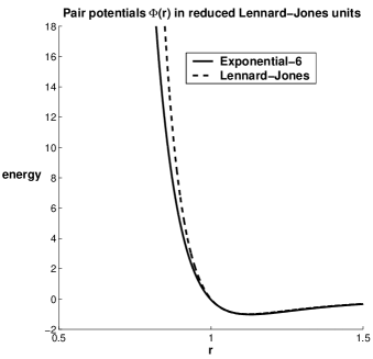
(a) Pair Potentials for Argon

(b) General form of the Lennard-Jones potential

Figure 2: (a): The Exp-6 pair potential is similar to the Lennard-Jones pair potential near the minimum, but the repulsion is slightly weaker in the Exp-6. The radius and the energy are measured in reduced Lennard-Jones units, where the Lennard-Jones parameters are $\epsilon_{\mathrm{LJ}}={k_{\mathrm{B}}}120\,\mathrm{K}$ and $\sigma_{\mathrm{LJ}}=3.405\,$Å.
(b): The parameter $\sigma_{\mathrm{LJ}}$ is the radius where the Lennard-Jones potential is 0, which is equal to the potential at infinite separation, and the parameter $\epsilon_{\mathrm{LJ}}$ is the depth of potential minimum.

Note that, while the Lennard–Jones pair potential tends to infinity as the interatomic distance tends to zero, the Exp-6 pair potential, as stated in (12), reaches a global maximum before turning down and approaching minus infinity in the limit. This clearly illustrates that the model based on the Exp-6 potential breaks down if two atoms come too close, but neither one of the pair potentials is designed to describe interactions of particles much closer than the typical nearest neighbour separation.

For short range potentials, like the Exp-6 and the Lennard-Jones potentials, the potential (and its derivative) decay sufficiently fast for the combined effect on the total potential energy (and the interatomic forces) of all atom pairs separated more than a certain distance to be negligible compared to the effect of the pairs separated less than the same distance. To take advantage of this in computations a cut-off radius is introduced and all interactions between particles separated by a distance larger than the cut-off are neglected; instead of summing over all $k\!\!\neq\!\!i$ in the inner sum in (11) the sum is only taken over particles in a spherical neighbourhood of particle $i$.

All the physical quantities in this report are given in the reduced Lennard-Jones units. Thus length is measured in units of $\sigma_{\mathrm{LJ}}$, energy in units of $\epsilon_{\mathrm{LJ}}$, and time in units of $\sqrt{m\sigma_{\mathrm{LJ}}^{2}/\epsilon_{\mathrm{LJ}}}$, where $m$ is the mass of one atom. (The time unit is the inverse of the characteristic frequency.) A list of the dimensionless units in the Argon model as well as the parameters in the Exp-6 potential can be found in Table 1. At the temperatures and pressures considered here, the stable phase of the Exp-6 potential is either the Face Centered Cubic (FCC) lattice or a liquid phase.

Quantity Unit Energy $1.6568\cdot 10^{-21}$ J Time $2.1557\cdot 10^{-12}$ s Mass $6.6412\cdot 10^{-26}$ kg Length $3.405\cdot 10^{-10}$ m Temperature $120$ K Pressure $4.1968\cdot 10^{7}$ Pa

Constant Value $k_{\mathrm{B}}$ 1 Parameter Value $A$ $3.84661\cdot 10^{5}$ $B$ $11.4974$ $C$ $3.9445$

Table 1: Atomic units and corresponding values of physical constants and parameters in the Exp-6 model (12). Non dimensional molecular dynamics equations are obtained after normalising with the atom mass, $m$, and the Lennard-Jones parameters, $\sigma_{\mathrm{LJ}}$ and $\epsilon_{\mathrm{LJ}}$; in this Argon model $m=6.6412\cdot 10^{-26}$ kg (or 39.948 atomic mass units), $\sigma_{\mathrm{LJ}}=3.405$ Å, and $\epsilon_{\mathrm{LJ}}/{k_{\mathrm{B}}}=120$ K, where $k_{\mathrm{B}}$ is the Boltzmann constant.

2.1.2 Newtonian System Simulated at Constant Pressure

The purpose here is to approximately determine the melting point at a high fixed pressure, to be able to set up and simulate stationary (FCC-liquid) two-phase systems later. Determination of the melting point follows the two-phase method described by Belonoshko and co-authors in [1].

The mathematical model

is a classical system of $N$ identical particles where the positions, ${X_{{\mbox{}}}^{t}}=({X_{1}^{t}},\ldots,{X_{{N}}^{t}})$, and the velocities, ${v_{\mbox{}}^{t}}=({v_{1}^{t}},\ldots,{v_{N}^{t}})$, evolve in time according to Newton’s equations

$$\frac{d{X_{{\mbox{}}}^{t}}}{dt} ={v_{\mbox{}}^{t}},$$ (13a)

$$\frac{d{v_{\mbox{}}^{t}}}{dt} =-\nabla_{{{X_{{\mbox{}}}^{{\mbox{}}}}}}{U}({X_{{\mbox{}}}^{t}}),$$ (13b)

where the total potential energy of the system is given by (11)-(12) using the parameter values in Table 1. Here $\nabla_{{{X_{{\mbox{}}}^{{\mbox{}}}}}}$ denotes the gradient with respect to the particle positions. The force acting on particle $i$ is $-\nabla_{{X_{i}^{{\mbox{}}}}}{U}({X_{{\mbox{}}}^{t}})$ and, since all particles have unit mass in the non-dimensional units, the acceleration is equal to the force. Particle positions are restricted to a finite computational box with periodic boundary conditions, corresponding to an infinite system where the same configuration of particles is repeated periodically in all three directions; a particle leaving the computational cell on one side enters the cell again from the opposite side and particles interact with periodic images of particles in the cell.

For a fixed volume of the computational cell the equations (13) will preserve the total energy, $E$, (the sum of potential and kinetic energy) of the system as well as the number of particles. It will approximately sample the $(N,V,E)$ ensemble. In the determination of the melting point the simulations are instead performed in an approximation of the $(N,T,P)$ ensemble, using a constant number of particles, $N$, a constant temperature, $T$, and a constant pressure, $P$. This must allow for the volume of the computational cell to change during the simulation. There must also be mechanisms for keeping the temperature and the pressure constant, thus modifying (13) so that the total energy varies.

Numerical computations

of the (N,T,P) molecular dynamic simulations were performed using Keith Refson’s publicly available software package Moldy, [9]. Constant temperature was enforced using the Nosé-Hoover thermostat, where the equations of motions (13) are modified, and extended, to include an additional degree of freedom modelling a thermal reservoir. The fictitious inertia associated with the thermal reservoir was $100\leavevmode\nobreak\ \mathrm{kJ}\,\mathrm{mol}^{-1}\,\mathrm{ps}^{2}$, corresponding to $21.57$ in the dimensionless equation. The pressure was kept constant using the Parinello-Rahman equation, controlling the dynamics of the vectors (three edges) that define the computational cell. The fictitious mass parameter in the Parinello-Rahman equation was $300\,\mathrm{amu}$ corresponding to $1.20\cdot 10^{4}$ in the reduced Lennard–Jones units. A short description of the Nosé-Hoover thermostat and the Parinello-Rahman equation, with references to papers with theoretical foundations of the methods, can be found in the manual [10].

The time stepping method in Moldy is a modification of Beeman’s algorithm using predictor-corrector iterations in the computation of the velocities; see [10] for details. The simulations described here used the constant time step $4.639\cdot 10^{-5}$ and the potential cut-off $2.937$.

In the two-phase method

for determination of the melting point the molecular dynamics simulation starts from an initial configuration that is part solid and part liquid. As the $({N},{T},{P})$ simulation proceeds the whole liquid part will solidify, if ${T}<{T_{\mathrm{M}}}$ for the given pressure, or the solid will melt, if ${T}>{T_{\mathrm{M}}}$, resulting in a single phase system. Starting from a coarse estimate of the temperature interval containing the melting temperature, that interval can be narrowed down by running simulations at temperatures in the interval and noting whether they equilibrate to an all solid or an all liquid system. The validity of this two-phase approach has been verified in [1] for determining, among other things, the melting point of a molecular dynamics model of Xenon, similar to the Argon model used here.

The initial configuration in a two-phase simulation was composed of pre-simulated solid and liquid configurations. The solid part was prepared by taking a perfect FCC configuration and performing a short molecular dynamics run at the temperature and pressure of the intended two-phase simulation to adapt the size of the computational cell.

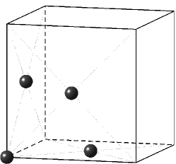
(a) The FCC unit cube

(b) Eight FCC unit cubes

Figure 3: A perfect FCC lattice consists of FCC unit cubes, (a), stacked next to each other in three dimensions, (b). With one atom in the $(0,0,0)$ corner of the unit cube the three other atoms are placed at the centres of the cubic faces intersecting in $(0,0,0)$.

Initially the sides of the computational cell were aligned with the sides of the unit cube in the perfect FCC lattice; see Figure 3. While in general the dynamics of the cell edges in the Parinello-Rahman equations allow the cell to take the shape of any parallelepiped, here the dynamics were restricted to only allow rescaling, without rotation, of the three edges and thus keeping the rectangular box shape of the cell. The preparation of the liquid part started from the configuration of the already prepared FCC-solid and a run was performed at a temperature well over the estimated melting point, where the sample would melt quickly; after equilibrating at the higher temperature the sample was quenched to the temperature of the two-phase simulation. Only one side of the computational cell was allowed to change while preparing the liquid part and thus the orthogonal cross section of the simulation cell was preserved from the FCC simulation. The solid and liquid parts were joined in the two-phase initial configuration by placing them next to each other, letting the cell faces of identical shape face each other. The general appearance is similar to the configurations shown in Figure 5 on page 5, even though those configurations belong to the constant volume Smoluchowski simulations where the set up procedure is slightly modified. Periodic boundary conditions were still applied in all directions, so that each part (solid or liquid) corresponded to a semi-infinite slab surrounded on two sides by the other phase with the effect of simulating a periodic, sandwiched, material. Voids of thickness of approximately one nearest neighbour separation were introduced in both solid–liquid interfaces to make sure that no pair of particles ended up to close in the initial configuration. Since the two-phase simulations were performed at constant pressure, the voids would fill in the beginning of the run as the length of the computational cell decreased.

In the two-phase simulations the lengths of all three vectors defining the cell edges were allowed to change. Starting from an initial two-phase configuration the molecular dynamics simulation was run until the system was considered equilibrated. After equilibration the computational cell was filled with either the solid or the liquid phase. The density of the FCC solid is higher than that of the liquid phase. If the phase change was solidification of the liquid, then the volume of the computational cell would decrease during the equilibration stage before assuming an approximately constant value; if the solid was melting, the total volume would grow during equilibration. The density of the stable phase at the given pressure and temperature was obtained by time averages of the simulation after equilibration.

When the volume per particle is shown as a function of the temperature, at constant pressure, it will display a sharp change at the melting point; see Figure 4(a) on page 4. The procedure will obtain an interval around the melting point and the accuracy can be improved by performing simulations at more temperatures to shorten the interval of uncertainty. However, the equilibration requires longer time when close to the melting point and the cost for refining the approximation grows, not only because the number of simulations grows, but more importantly because every single simulation takes longer to perform.

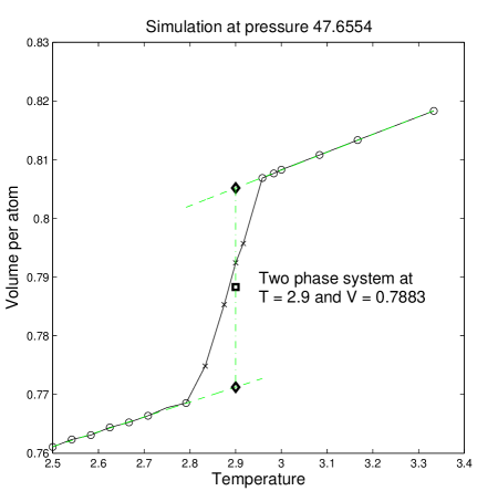
(a) Simulation data

(b) Extrapolated data at ${T}=2.9$

Figure 4: (a) Volume per atom as a function of temperature at a the pressure 47.6554 (or $2.0$ GPa) in $(N,P,T)$ simulations. Data points from simulations that are considered equilibrated are marked with $\circ$ and those from simulations that are not equilibrated are marked with $\times$. The two regions of equilibrated values where the volume per atom varies approximately linearly correspond to solid (FCC), at lower temperatures, and liquid, at higher temperature, respectively. The melting point at the given pressure is somewhere in between; the approximate value ${T}=2.9$ is used below and in the constant volume simulations.
(b) The volume per atom of solid and liquid have been extrapolated to ${T}=2.9$ by least square fits of straight lines to the simulation data and the corresponding number densities, $\rho$, have been computed. If ${T}=2.9$ is sufficiently close to the melting point at this pressure, then the two phases will coexist in constant volume, $(N,V,T)$, simulations provided that the total density is between the estimated densities of pure solid and pure liquid. The ratio of the volumes of the solid and the liquid part is determined by the total density of the combined system. The tabulated value of the density for a combined system gives approximately equal volumes of both parts at a pressure close to the one in the constant pressure simulations.

The main purpose here is to investigate the possibility of obtaining the model functions in a coarse grained phase-field model from $({N},{V},{T})$ Smoluchowski dynamics simulations, as described next. Therefor the accuracy in the determination of the melting point at the given pressure is critical only to the extent that it must be possible to perform the constant volume simulations at this temperature; that is, it must be possible to perform simulations on a two-phase system with stable interfaces between the solid and liquid parts. If the purpose were to perform computations at the melting point at this very pressure, then more computational effort would have to be spent on the accuracy of the melting point and the corresponding densities.

The numerical simulations were performed with ${N}=8000$ particles; the initial solid configuration consisted of 4000 particles, corresponding to $10\!\times\!10\!\times\!10$ FCC unit cells with four atoms each, and the liquid had the same number of particles. From simulations at the pressure 47.7 in the reduced Lennard-Jones units (corresponding to $2.0$ GPa) an approximate value of 2.9 for the melting point was obtained together with number densities for the liquid and solid extrapolated to this temperature; see Figure 4 on page 4. Fixing the temperature and the number density ${N}/{V}$, only one degree of freedom remains in the triple $({N},{V},{T})$, allowing the system size to vary.

2.1.3 Smoluchowski System Simulated at Constant Volume

The constant volume and temperature Smoluchowski dynamics two-phase simulations described here were used to compute the functions (10) defining the coarse-grained phase-field dynamics (7), as described in the introduction. This meant computing time averaged quantities like the time averaged potential energy phase-field (9) and the corresponding coarse-grained drift and diffusion coefficient functions (8).

The mathematical model

is that of $N$ particles whose positions ${X_{{\mbox{}}}^{t}}$ follow the Smoluchowski dynamics

$$d{X_{{\mbox{}}}^{t}} =-\nabla_{{{X_{{\mbox{}}}^{{\mbox{}}}}}}{U}({X_{{\mbox{}}}^{t}})\;dt+\sqrt{2{k_{\mathrm{B}}}{T}}\;dW^{t},$$ (14)

introduced on page 3. There are no velocities in the Smoluchowski dynamics. Instead the positions of all particles in the system give a complete description of the system at a particular time. Such a description, ${X_{{\mbox{}}}^{t}}$, will be refered to as a configuration of the system. The particles are contained in a computational cell, shaped like a rectangular box, of fixed dimensions and the boundary conditions are periodic in all directions. Hence the volume, $V$, and the number of particles, $N$, are fixed. Without velocities there is no kinetic energy, but the temperature, $T$, enters directly in the dynamics. The temperature parameter is held fixed, which can be viewed as a kind of thermostat built into the dynamics.

Since the volume of the computational cell is constant, unlike in the $({N},{T},{P})$ simulations above, the overall density of the system remains constant over time, which allows for stationary two-phase configurations where part of the domain is solid and part is liquid.

The numerical simulations

The discrete time approximations $\bar{X}_{{\mbox{}}}^{n}$ of $X_{{\mbox{}}}^{t_{n}}$, were computed using the explicit Euler-Maruyama scheme

$${\bar{X}_{{\mbox{}}}^{n}} ={\bar{X}_{{\mbox{}}}^{n-1}}-\nabla_{{{X_{{\mbox{}}}^{{\mbox{}}}}}}{U}({\bar{X}_{{\mbox{}}}^{n-1}})\;\Delta t^{n}+\sqrt{2{k_{\mathrm{B}}}{T}}\;\Delta W^{n},$$ (15)

where $\Delta t^{n}=t^{n}-t^{n-1}$ is a time increment and $\Delta W^{n}=W(t^{n})-W(t^{n-1})$ is an increment in the $3{N}$-dimensional Wiener process. Each run was performed using constant time step size, $\Delta t^{n}\equiv\Delta t$, but the time step could change between different runs depending on the purpose; in the equilibration phase the typical step size was $\Delta t=10^{-4}$, but in the production phase the step size had to be taken smaller, as discussed later.

The computation of $\nabla_{{{X_{{\mbox{}}}^{{\mbox{}}}}}}{U}({\bar{X}_{{\mbox{}}}^{n-1}})$ in every time step is potentially an $\mathcal{O}({N}^{2})$ operation since the potential is defined by pairwise interactions. The computations described here used the potential cut-off radius $3.0$, which meant that each particle only interacted directly with a relatively small number of neighbours (independent of $N$ since the density was approximately constant). To avoid the $\mathcal{O}({N}^{2})$ task of computing all pairwise distances in each time step, the computational cell is divided into smaller sub cells, where the size is defined in terms of the cut-off radius so that two particles only can interact if they are in the same sub cell or in two neighbouring sub cells; information about particles migrating between sub cells is exchanged in each time step. The computations use a two dimensional grid of sub cells, where the particle positions within each sub cell are sorted with respect to the third coordinate dimension in every time step. When the particles are sorted the sweep over all particles in a sub cell can be efficiently implemented and the sorting procedure is not too expensive since the particles do not move far in one time step. A more thorough description of this algorithm can be found in [13]. The actual code used here is a modification of a parallelised code for Newtonian molecular dynamics obtained from Måns Elenius in Dzugutov’s group[4]; the main modifications when adapting to Smoluchowski dynamics is the removal of velocities from the system and the introduction of a pseudo random number generator for the Brownian increments, $\Delta W^{n}$.

With the cut-off radius $3.0$ used in the computation and the model parameters in Table 1 on page 1, the Exp-6 pair potential and its derivatives are small at the cut-off radius. Still the potential will be discontinuous at the cut-off, unless it is slightly modified. A small linear term is added to make the potential continuously differentiable at the cut-off radius. In the practical computations, both the pair potential and the derivatives were obtained by linear interpolation from tabulated values.

The random number generator for normally distributed random variables was the Ziggurat method, described in [6], in a Fortran 90 implementation by Alan Miller, accessible from Netlib [7]. The underlying 32-bit integer pseudo random number generator is the 3-shift register SHR3. Since the purpose of the simulations only is to investigate if the coarse-graining procedure gives reasonable results just one pseudo random number generator was used, while several different random number generators ought to be used in a practical application. The generator was initialised with different seeds on different processors in the parallel computations, but it does not have distinct cycles simulating independent random variables. The hope is that the nature of the molecular dynamics simulations is enough to avoid the danger of correlated random numbers on the different processors, but this could be tested by comparing with other pseudo random generators that actually simulate independent random variables on different processors.

The two-phase systems

for the Smoluchowski dynamics simulations were set up to obtain a two-phase system at temperature ${T}=2.90$ with approximately equal volumes of solid and liquid and with stationary interfaces. To achieve this two equal volumes of FCC-solid and liquid were pre-simulated with the densities tabulated in Figure 4, on page 4. The preparation of the initial configurations for the Smoluchowski dynamics two-phase simulations was similar to the procedure described above, but some adjustments must be made because of the constant volume restriction. The shape of the computational cell used when generating the solid part was chosen to match the periodic structure of the FCC lattice at the tabulated density for the FCC part. A short equilibration run, at ${T}=2.90$, starting from a perfect FCC lattice at this density gave the initial solid configuration. The computational cell for the initial liquid part was chosen to be the same as the one in FCC simulation and the initial configuration when pre-simulating the liquid part was obtained from the FCC configuration by distributing vacancies to get the correct density in the liquid. In a simulation of (15) using a temperature, $T$, above the melting point, $T_{\mathrm{M}}$, the sample was melted and equilibrated. Afterwards the liquid was cooled to desired temperature using a subsequent simulation with ${T}={T_{\mathrm{M}}}$.

\begin{picture}(20.0,10.0)(0.0,0.0)\put(0.0,0.0){\makebox(0.0,0.0)[]{}} \end{picture}

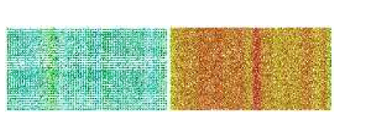
(a) Initial configuration, orientation 1

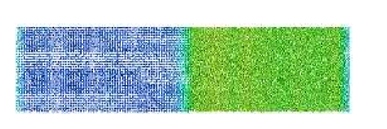
(b) Configuration at a later time, orientation 1

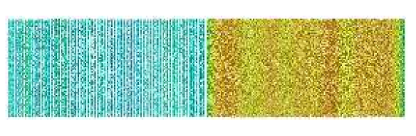
(c) Initial configuration, orientation 2

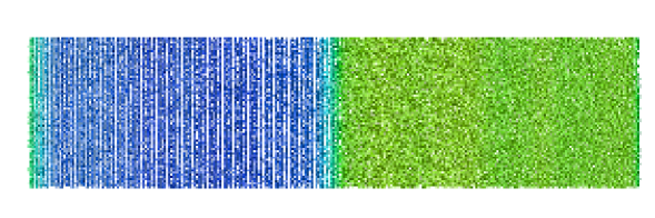
(d) Configuration at a later time, orientation 2

Figure 5: Snapshots of the process of setting up initial configurations for the two-phase simulations O1 and O2. The left part is solid (FCC) and the right part liquid. In the initial configurations, (a) and (c), the individual parts have been equilibrated at $T_{\mathrm{melt}}$ (for the combined system), and slightly compressed in one direction (to allow for two gaps). Subfigures (b) and (d) show configurations at later times when the parts have expanded to fill the voids and form two interfaces. The atoms are coloured according to a computed phase variable; in (a) and (b) the phase variable is just the instantaneous field ${m}(x_{1};{X_{{\mbox{}}}^{0}})$, whereas (b) and (d) use discrete time averages approximating $\frac{1}{t_{2}-t_{1}}\int_{t_{1}}^{t_{2}}{m}(x_{1};{X_{{\mbox{}}}^{t}})\,dt$.
 
Simulation O1 used 64131 particles in a computational cell of dimensions $93.17\times 23.29\times 23.29$, while simulation O2 used 78911 particles in a cell of dimensions $100.86\times 24.71\times 24.96$.

Since no pair of atoms can be too close in the initial configuration, gaps had to be introduced between the solid and liquid parts, but the voids could not be introduced as additional volumes in the computational cell; the individual parts were equilibrated at $(N,V,T)$ corresponding to the expected densities for solid and liquid in the combined system, so increasing the total volume would reduce the overall density, resulting in partial or total melting of the solid part. To make room for the voids both the solid and the liquid parts were compressed slightly in the direction normal to the solid–liquid interfaces, before inserting them in their respective volumes in the computational cell for the two-phase simulation. Initial configurations obtained by this procedure are shown as configurations (a) and (c) in Figure 5, on page 5. The orientation of the solid–liquid interfaces with respect to the FCC lattice differ between the two initial configurations shown, and these orientations with the corresponding numerical simulations will be labelled Orientation 1 (O1) and Orientation 2 (O2) in the following. The shaded plane in Figure 6(b) shows the orientation of the interface in O1 and the shaded plane in Figure 6(c) shows the orientation in O2.

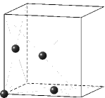
(a) Unit cell

(b) Orientation 1

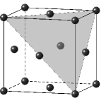
(c) Orientation 2

Figure 6: The shaded planes in (b) and (c) show the two orientations of the solid-liquid interface with respect to the FCC lattice treated in the numerical simulations.

Even though the compression in one direction was small, it introduced an artificial internal stress in the system. The higher value of the phase-field in the subfigures (a) and (c) in Figure 5 compared to the corresponding regions in the subfigures (b) and (d) is an effect of the compression. In the initial phase of the equilibration of the two-phase system, the compressed parts expand to fill the voids. The phase-fields in the interiors of the solid and liquid parts in subfigures (b) and (d) have reached the levels seen in the corresponding single phase systems, which shows at least that the local potential energy contributions had returned to normal before the production runs started.

As a test of the two-phase configuration serving as initial data in the production run, the radial distribution functions in the interior of the two phases were computed. The radial distribution function, $g(r)$, is useful for identifying the phase of a single-phase system. For a single component system $g(r)$, where $r\in\mathbb{R}^{+}$, is implicitly defined by the condition that the average number of atoms in a spherical shell between the radii $r_{1}$ and $r_{2}$ from the centre of any atom is

$${\rho}\int_{r_{1}}^{r_{2}}{g(r)}4\pi r^{2}\;dr,$$

where $\rho$ is the global particle density. In other words, the radial distribution function is the average particle density, as a function of the separation $r$, normalised by overall density. Figure 7, on page 7, shows good agreement for simulation O2 between $g(r)$ corresponding to single phase solid and liquid configurations and $g(r)$ computed in the interior of the two phases, excluding two intervals of length 10.0 in the interface regions.

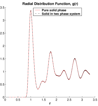
(a) FCC

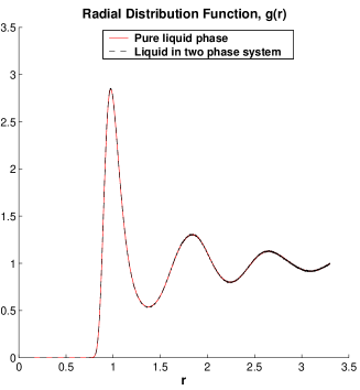
(b) Liquid

Figure 7: The radial distribution function, $g(r)$, computed from several configurations, separated in time, in the process of setting up the two-phase system in simulation O2. The solid curve shows $g(r)$ computed as an average over all particles in the computational cell used while pre-simulating the solid and the liquid part, in subfigure (a) and (b) respectively. The dashed curves show $g(r)$ computed as an average over particles in two slices of the computational cell of the two-phase system; subfigure (a) shows $g(r)$ obtained from the slice $5.0\leq x_{1}\leq 45.43$, inside the solid phase, and subfigure (b) shows $g(r)$ from the slice $55.43\leq x_{1}\leq 95.86$, inside the liquid phase. The configurations are taken from an equilibration run, after the closing of the initial gaps between the pre-simulated phases, but before the “production” run. The radial distribution functions show good agreement between the single phase systems and the corresponding solid and liquid subdomains away from the interface.

An effect of the finite size of the computational cell is that periodic boundary conditions may interact with the solid and affect the results; here the computational cell was chosen to match the FCC structure in a specific orientation with respect to the box and thus stabilises the structure and orientation. It is important to know that the density in the FCC part (and hence the box cross section) is consistent with constant pressure simulations close to the melting point. A related question is whether the length of the computational box is large enough for properties around the interfaces in the infinitely layered structure to be good approximations of those near an interface between a solid and liquid on the macroscopic scale.

2.2 Computation Of the Coarse-Grained Model Functions

The coefficient functions (10) in the stochastic differential equation (7) for the coarse-grained phase-field are defined in terms of the time averaged expected values (8) and (9) on the form

$$\frac{1}{{\mathcal{T}}}{\mathrm{E}}\left[\int_{0}^{\mathcal{T}}\psi(\cdot;{{X_{{\mbox{}}}^{t}}})\;\bigg{|}\;{X_{{\mbox{}}}^{0}}={X_{0}^{{\mbox{}}}}\right],$$

where ${X_{0}^{{\mbox{}}}}$ is a configuration of a stationary two-phase system. By setting up an initial configuration, ${X_{0}^{{\mbox{}}}}$, as described in the previous section, and simulating discrete sample trajectories using the Euler-Maruyama method (15), a sequence of configurations $\{{\bar{X}_{{\mbox{}}}^{k}}\}_{k=1}^{K}$ approximating the sequence $\{{X_{{\mbox{}}}^{t_{k}}}\}_{k=1}^{K}$ for some times $0<t_{1}<\cdots<t_{K}={\mathcal{T}}$, is obtained. In a post processing step a set of configurations ${\mathcal{S}}\subseteq\{{\bar{X}_{{\mbox{}}}^{k}}\}_{k=1}^{K}$ is selected and averages

$${\mathcal{A}_{{\mathcal{S}}}\left(\psi\right)} =\sum_{{{X_{{\mbox{}}}^{{\mbox{}}}}}\in{\mathcal{S}}}\psi(\cdot;{{{X_{{\mbox{}}}^{{\mbox{}}}}}})w_{{X_{{\mbox{}}}^{{\mbox{}}}}},$$

consistently weighted with weights $w_{{X_{{\mbox{}}}^{{\mbox{}}}}}$, are computed as approximations of the corresponding expected values in the continuous time model. It is usually more efficient not to include every configuration in the averages. This will be discussed in Section 3.

As described in the introduction, the averages are functions of the coordinate direction $x_{1}$, normal to the planar interface, since the mollifier in the definition (5) of the microscale phase-field, $m$, is chosen to take uniform averages in the planes parallel to the interface. The mollifier used in the computations is

$${\eta}(x) ={\eta}(x_{1})=c\exp{\left(-\frac{1}{2}\left(\frac{x_{1}}{\epsilon}\right)^{2}\right)}{\mathbf{1}_{|x_{1}|<R_{c}}},$$ (16)

where $c$ is a normalising constant, $\epsilon$ is a smoothing parameter, and $R_{c}$ is a cut-off. The smoothing parameter is on the order of typical nearest neighbour distances, ${\epsilon}\approx 1$, and $R_{c}=6{\epsilon}$, for all choices of $\epsilon$, which gives ${\eta}(R_{c})\approx 1.5\cdot 10^{-8}{\eta}(0)$; the shape of $\eta$ can be seen in Figure 25(a), on page 25(a).

An explicit derivation of expressions for the drift and the diffusion is given in Appendix A. Separating the drift in terms containing two, one, and zero, derivatives of the mollifier, the right hand side of (8a) is approximated by

$${k_{\mathrm{B}}}{T}\frac{\partial^{2}}{\partial x_{1}^{2}}{\mathcal{A}_{{\mathcal{S}}}\left({m}\right)}+\frac{\partial}{\partial x_{1}}{\mathcal{A}_{{\mathcal{S}}}\left({a_{1}}\right)}+{\mathcal{A}_{{\mathcal{S}}}\left({a_{0}}\right)},$$

where

$${a_{1}}(x;{{X_{{\mbox{}}}^{{\mbox{}}}}}) ={\sum_{j=1}^{N}}({k_{\mathrm{B}}}{T}-{m_{j}}({{X_{{\mbox{}}}^{{\mbox{}}}}}))[{F}_{j}({{X_{{\mbox{}}}^{{\mbox{}}}}})]_{1}{\eta}(x-{X_{j}^{{\mbox{}}}})$$ (17)

and

$${a_{0}}(x;{{X_{{\mbox{}}}^{{\mbox{}}}}}) =-{\sum_{j=1}^{N}}\left({k_{\mathrm{B}}}{T}\nabla_{X_{j}}\cdot{F}_{j}({{X_{{\mbox{}}}^{{\mbox{}}}}})+\frac{1}{2}||{F}_{j}({{X_{{\mbox{}}}^{{\mbox{}}}}})||^{2}\right){\eta}(x-{X_{j}^{{\mbox{}}}})$$

$$\quad-\frac{1}{2}{\sum_{j=1}^{N}}{\sum_{i\neq j,i=1}^{N}}{f}_{ij}({{X_{{\mbox{}}}^{{\mbox{}}}}})\cdot{F}_{j}({{X_{{\mbox{}}}^{{\mbox{}}}}}){\eta}(x-{X_{i}^{{\mbox{}}}}).$$ (18)

Here ${F}_{j}$ is the total force acting on particle $j$, $[{F}_{j}({{X_{{\mbox{}}}^{{\mbox{}}}}})]_{1}$ is the $x_{1}$-component of the force, and ${f}_{ij}$ are the contributions from individual pairs,

$${F}_{j}({{X_{{\mbox{}}}^{{\mbox{}}}}})=-\nabla_{X_{j}}{U}({{X_{{\mbox{}}}^{{\mbox{}}}}}) ={\sum_{i\neq j,i=1}^{N}}{\Phi}^{\prime}(||{X_{i}^{{\mbox{}}}}-{X_{j}^{{\mbox{}}}}||)\frac{{X_{i}^{{\mbox{}}}}-{X_{j}^{{\mbox{}}}}}{||{X_{i}^{{\mbox{}}}}-{X_{j}^{{\mbox{}}}}||}={\sum_{i\neq j,i=1}^{N}}{f}_{ij}({{X_{{\mbox{}}}^{{\mbox{}}}}}).$$

The right hand side in equation (8b), for the coarse grained diffusion, is approximated by

$${\overline{B}}(\cdot,\cdot) ={\mathcal{A}_{{\mathcal{S}}}\left(2{k_{\mathrm{B}}}{T}{\sum_{j=1}^{N}}\bigl{(}p_{j}(\cdot,\cdot;X)+q_{j}(\cdot,\cdot;X)\bigr{)}\right)},$$ (19)

where

$$p_{j}(x,y;{{X_{{\mbox{}}}^{{\mbox{}}}}}) =\left(\frac{{m_{j}}({{X_{{\mbox{}}}^{{\mbox{}}}}})}{\epsilon^{2}}\right)^{2}\left[x-{X_{j}^{{\mbox{}}}}\right]_{1}\left[y-{X_{j}^{{\mbox{}}}}\right]_{1}{\eta}(x-{X_{j}^{{\mbox{}}}}){\eta}(y-{X_{j}^{{\mbox{}}}})$$

$$\quad-\frac{{m_{j}}({{X_{{\mbox{}}}^{{\mbox{}}}}})}{2\epsilon^{2}}[x-{X_{j}^{{\mbox{}}}}]_{1}{\eta}(x-{X_{j}^{{\mbox{}}}})\biggl{(}[{F}_{j}({{X_{{\mbox{}}}^{{\mbox{}}}}})]_{1}{\eta}(y-{X_{j}^{{\mbox{}}}})+\!\!{\sum_{i\neq j,i=1}^{N}}[{f}_{ij}({{X_{{\mbox{}}}^{{\mbox{}}}}})]_{1}{\eta}(y-{X_{i}^{{\mbox{}}}})\biggr{)}$$

$$\quad-\frac{{m_{j}}({{X_{{\mbox{}}}^{{\mbox{}}}}})}{2\epsilon^{2}}[y-{X_{j}^{{\mbox{}}}}]_{1}{\eta}(y-{X_{j}^{{\mbox{}}}})\biggl{(}[{F}_{j}({{X_{{\mbox{}}}^{{\mbox{}}}}})]_{1}{\eta}(x-{X_{j}^{{\mbox{}}}})+\!\!{\sum_{i\neq j,i=1}^{N}}[{f}_{ij}({{X_{{\mbox{}}}^{{\mbox{}}}}})]_{1}{\eta}(x-{X_{i}^{{\mbox{}}}})\biggr{)}$$

and

$$q_{j}(x,y;{{X_{{\mbox{}}}^{{\mbox{}}}}}) =\frac{1}{4}\biggl{(}{F}_{j}({{X_{{\mbox{}}}^{{\mbox{}}}}}){\eta}(x-{X_{j}^{{\mbox{}}}})+{\sum_{i\neq j,i=1}^{N}}{f}_{ij}({{X_{{\mbox{}}}^{{\mbox{}}}}}){\eta}(x-{X_{i}^{{\mbox{}}}})\biggr{)}$$

$$\quad\quad\cdot\biggl{(}{F}_{j}({{X_{{\mbox{}}}^{{\mbox{}}}}}){\eta}(y-{X_{j}^{{\mbox{}}}})+{\sum_{i\neq j,i=1}^{N}}{f}_{ij}({{X_{{\mbox{}}}^{{\mbox{}}}}}){\eta}(y-{X_{i}^{{\mbox{}}}})\biggr{)}.$$

The functions ${\mathcal{A}_{{\mathcal{S}}}\left(\psi\right)}$ are computed in a discrete set of points $D_{K}=\{x_{1}^{i}\}_{i=1}^{K}$ along the $x_{1}$ axis of the molecular dynamics domain. This makes the computed components, ${\mathcal{A}_{{\mathcal{S}}}\left({m}\right)}$, ${\mathcal{A}_{{\mathcal{S}}}\left({a_{1}}\right)}$, and ${\mathcal{A}_{{\mathcal{S}}}\left({a_{0}}\right)}$, of the drift coefficient function $K$-vectors and the computed $\overline{B}$ a $K$-by-$K$ matrix. The individual diffusion coefficient functions ${\overline{b}}_{j}$ are obtained by taking the square root of the computed diffusion matrix, ${\overline{B}}={\overline{B}}^{1/2}{({\overline{B}}^{1/2})^{\mathrm{T}}}$, and letting the $j$:th column of ${\overline{B}}^{1/2}$ define ${\overline{b}}_{j}$. While an exact computation would produce a symmetric positive semi definite matrix $\overline{B}$, finite precision effects make some computed eigenvalues negative, but small in absolute value. In an eigenvector factorisation of $\overline{B}$, let ${\Lambda}$ denote a diagonal matrix with all eigenvalues of $\overline{B}$ and ${\Lambda_{+}}$ a smaller diagonal matrix containing the dominant, possibly all, of the positive eigenvalues but no negative ones. Let ${V}$ and ${V_{+}}$ be the matrices of the corresponding eigenvectors. Then the square root of the matrix ${\Lambda_{+}}$ is a real diagonal matrix which can be used in the approximation

$${\overline{B}} ={V}{\Lambda}{{V}^{\mathrm{T}}}\approx{V_{+}}{\Lambda_{+}}{{V_{+}}^{\mathrm{T}}}=\left({V_{+}}{\Lambda_{+}}^{1/2}{{V_{+}}^{\mathrm{T}}}\right){\left({V_{+}}{\Lambda_{+}}^{1/2}{{V_{+}}^{\mathrm{T}}}\right)^{\mathrm{T}}}=\colon\;{B}{{B}^{\mathrm{T}}}.$$ (20)

With one Wiener process ${\widetilde{W}}_{j}$ in the coarse-grained stochastic differential equation (7) per evaluation point, $K={M}$, the component vectors, ${\overline{b}}_{j}$, of the diffusion in coarse-grained equation can be defined as the column vectors of the matrix $B$, to obtain

$${\sum_{j=1}^{M}}{\overline{b}}_{j}{{\overline{b}}_{j}^{\mathrm{T}}} \approx{\overline{B}}.$$

If two grid points, $x_{1}$ and $y_{1}$, are further apart than twice the sum of the cut-off in the potential and the cut-off in the mollifier, then $p_{j}(x,y;\cdot)$ and $q_{j}(x,y;\cdot)$ is zero; hence a natural ordering $x_{1}^{1}<x_{1}^{2}<\cdots<x_{1}^{K}$ of the grid points makes $\overline{B}$ a band matrix. The definition of $B$ in (20) preserves the connection between grid points and diffusion functions and the dominating terms in a tabulated vector ${\overline{b}}_{j}$ are those of nearby grid points.

3 Results

This section describes results from numerical simulations performed to compute the coarse-grained model functions. The value of the smoothing parameter $\epsilon$ in the mollifier is $1.0$, unless another value is specified.

3.1 The averaged phase-field ${m}_{\mathrm{av}}\approx{\mathcal{A}_{{\mathcal{S}}}\left({m}\right)}$

The first observation is that during the time intervals of the molecular dynamics simulations, the interfaces between the solid and the liquid subdomains were sufficiently stable for the averaged potential energy phase-fields, ${\mathcal{A}_{{\mathcal{S}}}\left({m}\right)}$, to appear qualitatively right. The phase-field appears to have two distinct equilibrium values, corresponding to the solid and liquid subdomains, and the transitions between the two regions are smooth and occur over distances of a few nearest neighbour distances; see Figure 8. Figure 9(b) shows that the computational cells in the molecular dynamics simulations are large enough for the phase-field in the interior of the two phases to attain values similar to the values in the corresponding single phase simulations. In simulations with a cubic, $23.29\times 23.29\times 23.29$, computational cell the gap between the phase-field levels in the solid and the liquid was significantly smaller, which indicates that the length of the computational cell can not be taken much smaller than in simulations O1 and O2. It is still possible that further increasing the size of the computational cell may affect the results.

(a) Orientation 1

(b) Orientation 1

(c) Orientation 2

(d) Orientation 2

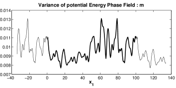
(e) Orientation 2

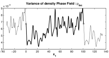
(f) Orientation 2

Figure 8: Subfigures (a) and (c) show the potential energy phase-field, ${\mathcal{A}_{{\mathcal{S}}}\left({m}\right)}$, computed from simulations O1 and O2, respectively. Subfigures (b) and (d) show the corresponding spatially averaged particle densities. Subfigures (e) and (f) show the pointwise sample variance associated with the averages in (c) and (d). The thick parts of the curves show the computed functions in molecular dynamics cell. The thinner parts show the periodic continuations across the boundaries of the cell, marked by circles. The averages in simulation O1, and O2, were formed over 1721, and 1775, configurations separated in time by $5\cdot 10^{-4}$, so that the total time from first to last configuration was 0.860, and 0.8875, respectively. The high frequency fluctuations are small after averaging on this time scale, but larger fluctuations remain in both phases. This suggests that the two phase system is not yet equilibrated. Still the computed phase-fields appear qualitatively correct.

(a) Density Phase-Field, O2

(b) Potential Energy Phase-Field, O2

Figure 9: The computational cell in the molecular dynamics simulations must be sufficiently large for the infinitely layered structure to resemble a system with a single solid–liquid interface on the macroscopic scale. In simulation O2 the total length of the computational cell was 100.86; subfigure (b) shows that this was sufficient for the averaged phase-field, ${\mathcal{A}_{{\mathcal{S}}}\left({m}\right)}$, to obtain values in the interior of each phase that are similar to the functions, marked by thick curves, obtained in the single phase configurations simulated during the setup of simulation O2.

3.2 The averaged drift ${\overline{a}}\approx{\mathcal{A}_{{\mathcal{S}}}\left({\alpha}\right)}$

The average ${\mathcal{A}_{{\mathcal{S}}}\left({m}\right)}$ approximates the expected time average (9). The next expected value to study is the one defining the coarse grained drift in (8a). In a stationary situation, where the interfaces do not move during the simulation and the averaged phase-field converges to a stationary profile, the average total drift in the stochastic differential equation describing the phase-field variable must converge to zero. Still the time averaged total drift corresponding to the simulation O2, whose averaged phase-field was discussed above, is far from zero; see Figure 10. The computed time averaged drift

$${\mathcal{A}_{{\mathcal{S}}}\left({\alpha}(x;{\bar{X}_{{\mbox{}}}^{n}})\right)} \approx\frac{1}{{\mathcal{T}}}{\mathrm{E}}\biggl{[}\int_{0}^{\mathcal{T}}{\alpha}(x;{X_{{\mbox{}}}^{t}})\,dt\;\Bigl{\lvert}\;{X_{{\mbox{}}}^{0}}={X_{0}^{{\mbox{}}}}\biggr{]}$$

depends both on the length of the time interval where the average is computed, the number of configurations used in the average, and on the discrete approximation $\bar{X}_{{\mbox{}}}^{n}$ of $X_{{\mbox{}}}^{t_{n}}$; these potential error sources must be analysed to explain the result.

Figure 10: The average total drift, ${\mathcal{A}_{{\mathcal{S}}}\left({\alpha}\right)}$, based on the same 1775 configurations from simulation O2 as ${\mathcal{A}_{{\mathcal{S}}}\left({m}\right)}$ in Figure 8(c), is still dominated by large oscillations.

3.2.1 The effect of discrete time dynamics

First consider the error associated with the discrete dynamics. The explicit form of the drift is derived for the continuous time mathematical model with the Smoluchowski dynamics (14), and not the discrete time Euler-Maruyama dynamics (15) that is used in the numerical simulations. For a fixed size of the time step this means that, even if the state of the numerical simulation is stationary on the time scale of the simulation so that time averaged phase-field converges to an equilibrium profile, the time averaged total drift will not go zero because of the time discretisation error. Figure 11 shows that the computed radial distribution functions, here from single phase solid configurations, are close when the time steps used vary from $10^{-7}$ to $10^{-4}$; still the larger time steps give average computed drifts ${\mathcal{A}_{{\mathcal{S}}}\left({\alpha}(x;{\bar{X}_{{\mbox{}}}^{n}})\right)}$ that are inconsistent with the observed time evolution of the average phase-field ${\mathcal{A}_{{\mathcal{S}}}\left({m}(x;{\bar{X}_{{\mbox{}}}^{n}})\right)}$. As shown in Figure 13, the time step $\Delta t=1\cdot 10^{-5}$ gives an average drift that oscillates between -100 and -250, even when the computed phase-field ${\mathcal{A}_{{\mathcal{S}}}\left({m}(x;{\bar{X}_{{\mbox{}}}^{n}})\right)}$ is approximately constant over times of the order 10. For this reason, the time step used in simulations O1 and O2, generating configurations for the computation of ${\mathcal{A}_{{\mathcal{S}}}\left({m}(x;{\bar{X}_{{\mbox{}}}^{n}})\right)}$ and ${\mathcal{A}_{{\mathcal{S}}}\left({\alpha}(x;{\bar{X}_{{\mbox{}}}^{n}})\right)}$, was $\Delta t=5\cdot 10^{-7}$ , while the time step used in the setup of the initial configurations often was a thousand times larger. With this small time step the fluctuations in the computed average drift outweighs the deviation from the expected zero mean; see Figure 10.

The choice of the time step size $\Delta t=5\cdot 10^{-7}$ was guided by a rough error estimate, taking into account the maximal absolute value of second order derivatives of the Smoluchowski drift $-\nabla_{X_{j}}{U}({X_{{\mbox{}}}^{t}})$ when the nearest neighbours don’t come closer than approximately 0.8, as indicated by Figure 11. Then the time step was adjusted so that the slow convergence of the time averaged drift in terms of $\mathcal{T}$ and the number of configurations, $\bar{X}_{{\mbox{}}}^{n}$, was the dominating error source in the results. This over-killing of the time discretisation error in the molecular dynamics wastes computer power and could possibly be avoided by more accurate error estimates, allowing a matching of the different error contributions. Using a reasonable number of grid points, $K$, in the computation of the drift coefficient $K$-vectors and the diffusion $K$-by-$K$ matrix $\overline{B}$, in (19), the computational cost for obtaining $\overline{B}$ in particular, far exceeds the cost of actually making a time step in the molecular dynamics simulation. Hence the additional cost of over-killing the time step error is not very significant, provided that not every configuration in the time stepping is included in the averages $\mathcal{A}_{{\mathcal{S}}}\left({m}\right)$, $\mathcal{A}_{{\mathcal{S}}}\left({\alpha}\right)$, and $\overline{B}$. In the averages shown in Figure 8 and Figure 10, for example, the configurations were sampled at time intervals $5\cdot 10^{-4}$, corresponding to 1000 time steps in the molecular dynamics simulation.

A further improvement may be to incorporate finite step-size effects in the expressions for the components of the drift. The higher order derivatives of the pair potential attain large values when two particles come closer than 1; see Figure 12. Hence the time step must be taken very small for Itô’s formula to be a good approximation of the dynamics of the discrete system. Instead of a direct application of Itô’s formula in the derivation of the drift and diffusion terms in (26) and (27) on page 26 one could include higher order terms in the expansion to improve the accuracy of the computed drift.

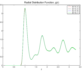
(a) $g(r)$, FCC, different $\Delta t$

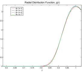
(b) Detail: first slope

Figure 11: The radial distribution function, $g(r)$, computed using four different step sizes in a single phase FCC simulation. The difference between the curves is small (a), even if the one obtained for $\Delta t=10^{-4}$ differs visibly from the others in the first peak (b). In spite of the good approximation in the radial distribution function, the larger step sizes give very poor results in the computed dynamics of $m$.

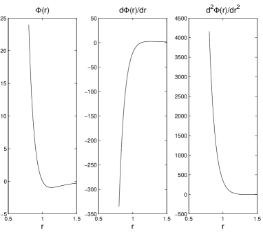
Figure 12: The absolute value of the Exp-6 potential and its derivatives grow very quickly with decreasing $r$, in the range with positive $g(r)$ in Figure 11(b). The potential and its two first derivatives using the model parameters in Table 1, on page 1, are shown here.

(a) ${\mathcal{A}_{{\mathcal{S}}}\left({m}\right)}$

(b) ${\mathcal{A}_{{\mathcal{S}}}\left({\alpha}\right)}$

(c) ${\mathcal{A}_{{\mathcal{S}}}\left({a_{1}}\right)}$

(d) ${\mathcal{A}_{{\mathcal{S}}}\left({a_{0}}\right)}$

(e) ${k_{\mathrm{B}}}{T}\frac{\partial^{2}}{\partial x_{1}^{2}}{\mathcal{A}_{{\mathcal{S}}}\left({m}\right)}$

Figure 13: Using the step size $\Delta t=1\cdot 10^{-5}$ in the Euler-Maruyama scheme, the computed average phase-field ${\mathcal{A}_{{\mathcal{S}}}\left({m}\right)}$ is approximately stationary during the time interval of the averaging. In subfigure (a) the average is based on 123 configurations, sampled at every ten thousandth time step, corresponding to a total time interval of 12.3. Still, the computed average drift ${\mathcal{A}_{{\mathcal{S}}}\left({\alpha}\right)}$ is far from zero during this time interval. The large deviation from zero is entirely due to the term ${\mathcal{A}_{{\mathcal{S}}}\left({a_{0}}\right)}$.

(a) Mean based on 111 configurations, ${\mathcal{T}}=0.0555$

(b) Mean based on 444 configurations, ${\mathcal{T}}=0.2220$

(c) Mean based on 1775 configurations, ${\mathcal{T}}=0.8875$

	${\mathcal{T}}=0.0555$	${\mathcal{T}}=0.2220$	${\mathcal{T}}=0.8750$
111 cfgs.	-5.7 ($1.3\cdot 10^{3}$)	-10.3 ($1.2\cdot 10^{3}$)	4.3 ($1.1\cdot 10^{3}$)
444 cfgs.		6.1 ($2.1\cdot 10^{2}$)	0.67 ($2.7\cdot 10^{2}$)
1775 cfgs.			1.9 ($3.8\cdot 10^{1}$)

(d) The spatial ($x_{1}$) mean and, within parentheses, variance of ${\mathcal{A}_{{\mathcal{S}}}\left({\alpha}\right)}$

Figure 14: The total drift ${\mathcal{A}_{{\mathcal{S}}}\left({\alpha}\right)}$, decays slightly faster with $\mathcal{T}$ than the predicted $1/\sqrt{{\mathcal{T}}}$ in the examples (a), (b), and (c) above. Here the number of configurations in the averages grows with $\mathcal{T}$ and the means and variances of ${\mathcal{A}_{{\mathcal{S}}}\left({\alpha}\right)}$ tabulated in (d) suggest that the number of configurations still restricts the rate of convergence. The average in subfigure (c) is based on the same 1775 configurations from simulation O2 as ${\mathcal{A}_{{\mathcal{S}}}\left({m}\right)}$ in Figure 8(c). The averages in subfigures (a) and (b) are based on the first 111 and 444 configurations, respectively.

3.2.2 Dependence on the length of the time averaging interval

Next consider the dependence of the computed coarse-grained drift coefficient function on the length of the time interval $\mathcal{T}$. Introducing the time averaged drift over a sample path as

$${\overline{A}}_{\mathcal{T}} =\frac{1}{{\mathcal{T}}}\int_{0}^{\mathcal{T}}{\alpha}(\cdot;{X_{{\mbox{}}}^{t}})\;dt,$$

the coarse-grained drift (8a) is ${\overline{a}}={\mathrm{E}}[{\overline{A}}_{\mathcal{T}}]$. The rate of convergence of ${\overline{a}}$, as ${\mathcal{T}}\to\infty$, in the continuous time mathematical model can be estimated by integration of the stochastic differential equation (6) for the phase-field $m$. Integrating from 0 to $\mathcal{T}$ gives

$${m}(\cdot;{X_{{\mbox{}}}^{{\mathcal{T}}}})-{m}(\cdot;{X_{{\mbox{}}}^{0}}) =\int_{0}^{\mathcal{T}}{\alpha}(\cdot;{X_{{\mbox{}}}^{t}})\;dt+\int_{0}^{\mathcal{T}}{\sum_{j=1}^{N}}\sum_{k=1}^{3}{\beta}_{j,k}(\cdot;{X_{{\mbox{}}}^{t}})\;dW_{j,k}^{t},$$ (21)

so that, by taking the expectation and using that, since $X_{{\mbox{}}}^{t}$ is $W^{t}$-adapted, the expectations of the Itô-integrals vanish

$${\mathrm{E}}\left[\int_{0}^{\mathcal{T}}{\alpha}(\cdot;{X_{{\mbox{}}}^{t}})\;dt\right] ={\mathrm{E}}\left[{m}(\cdot;{X_{{\mbox{}}}^{{\mathcal{T}}}})-{m}(\cdot;{X_{{\mbox{}}}^{0}})\right].$$ (22)

Hence, if the phase-field is stationary, then the expected mean drift over time is zero. Normalising (21) and (22) by $\mathcal{T}$,

$${\overline{A}}_{\mathcal{T}}-{\mathrm{E}}\left[{\overline{A}}_{\mathcal{T}}\right]=\\ \frac{1}{{\mathcal{T}}}\left({m}(\cdot;{X_{{\mbox{}}}^{{\mathcal{T}}}})-{m}(\cdot;{X_{{\mbox{}}}^{0}})-{\mathrm{E}}\left[{m}(\cdot;{X_{{\mbox{}}}^{{\mathcal{T}}}})-{m}(\cdot;{X_{{\mbox{}}}^{0}})\right]-{\sum_{j=1}^{N}}\sum_{k=1}^{3}\int_{0}^{\mathcal{T}}{\beta}_{j,k}(\cdot;{X_{{\mbox{}}}^{t}})\;dW_{j,k}^{t}\right)$$

and the variance of ${\overline{A}}_{\mathcal{T}}$ is obtained as

$${\mathrm{Var}}[{\overline{A}}_{\mathcal{T}}] ={\mathrm{E}}\left[\left({\overline{A}}_{\mathcal{T}}-{\mathrm{E}}\left[{\overline{A}}_{\mathcal{T}}\right]\right)^{2}\right]$$

$$=\frac{1}{{\mathcal{T}}^{2}}{\mathrm{Var}}\biggl{[}{m}(\cdot;{X_{{\mbox{}}}^{{\mathcal{T}}}})-{m}(\cdot;{X_{{\mbox{}}}^{0}})\biggr{]}$$

$$\quad+\frac{1}{{\mathcal{T}}^{2}}{\sum_{j=1}^{N}}\sum_{k=1}^{3}{\mathrm{E}}\left[\left(\int_{0}^{\mathcal{T}}{\beta}_{j,k}(\cdot;{X_{{\mbox{}}}^{t}})\;dW_{j,k}^{t},\right)^{2}\right]$$

$$\quad-\frac{2}{{\mathcal{T}}^{2}}{\mathrm{E}}\left[\bigl{(}{m}(\cdot;{X_{{\mbox{}}}^{{\mathcal{T}}}})-{m}(\cdot;{X_{{\mbox{}}}^{0}})\bigr{)}\left({\sum_{j=1}^{N}}\sum_{k=1}^{3}\int_{0}^{\mathcal{T}}{\beta}_{j,k}(\cdot;{X_{{\mbox{}}}^{t}})\;dW_{j,k}^{t}\right)\right],$$

where last expression was simplified using the independence of the different components of $W^{t}$, and the zero expected value of Itô integrals. Assuming that both the phase-field and all the diffusion coefficients are bounded, the dominating term in the expression for the variance is

$$\frac{1}{{\mathcal{T}}^{2}}{\sum_{j=1}^{N}}\sum_{k=1}^{3}{\mathrm{E}}\left[\left(\int_{0}^{\mathcal{T}}{\beta}_{j,k}(\cdot;{X_{{\mbox{}}}^{t}})\;dW_{j,k}^{t},\right)^{2}\right] =\mathcal{O}\left(\frac{1}{{\mathcal{T}}}\right).$$

In the two phase simulations considered here, the values of the computed phase-field varies between a lower level in the solid a higher in the liquid. Because of the small positive probability for two particles, with trajectories computed using the Euler-Maruyama dynamics (15), to get within an arbitrarily small distance of each other, there is no guarantee that computed phase-field always will stay in this range. However, if the minimum interatomic distance becomes to small, that is a breakdown of the whole microscopic model and not just a problem when computing the drift; this situation has not been observed to happen in the simulations here and the observed values of the phase-field are all in the range $(-1.5,1.0)$. Hence the assumption that $m$ is bounded seems reasonable here; a bound on the absolute value of the diffusion coefficients ${\beta}_{j,k}$ is less certain, and it will have to be larger than the bound on $m$.

For the average drift to be small compared to the stationary values of the phase-field itself, it must be at least a factor 100 smaller than the computed average shown in Figure 10. Based on the rough analysis above, the expected time average of the total drift can be expected to decay as $1/\sqrt{{\mathcal{T}}}$ with a large constant factor. When the computed drift $\mathcal{A}_{{\mathcal{S}}}\left({\alpha}\right)$ in Figure 10 is compared to averages computed using two smaller subsequences of configurations, the convergence to zero appears to be slightly faster than $1/\sqrt{{\mathcal{T}}}$; see Figure 14. Even when extrapolating with the measured convergence rate, decreasing the average drift by a factor 100 would require increasing the averaging time interval by more than a factor 1000, which is beyond reach within the present project. With increasing accuracy in the time average, eventually the time step in the molecular dynamics simulations must be decreased, further increasing the computational cost.

Since the total drift coefficient function, ${\overline{a}}(x_{1})\approx{\mathcal{A}_{{\mathcal{S}}}\left({\alpha}(x_{1};\cdot)\right)}$, where

$${\mathcal{A}_{{\mathcal{S}}}\left({\alpha}(x_{1};\cdot)\right)} ={k_{\mathrm{B}}}{T}\frac{\partial^{2}}{\partial x_{1}^{2}}{\mathcal{A}_{{\mathcal{S}}}\left({m}(x_{1};\cdot)\right)}+\frac{\partial}{\partial x_{1}}{\mathcal{A}_{{\mathcal{S}}}\left({a_{1}}(x_{1};\cdot)\right)}+{\mathcal{A}_{{\mathcal{S}}}\left({a_{0}}(x_{1};\cdot)\right)},$$ (23)

in the coarse grained model is expected to be zero in a stationary situation, a more accurate computation would serve primarily as a consistency test. On the other hand, the individual terms in the right hand side are not all expected to vanish independently. Indeed, it is clear from the results on $\mathcal{A}_{{\mathcal{S}}}\left({m}(x_{1};\cdot)\right)$ in Section 3.1 that the term with two differentiations with respect to $x_{1}$ will not be identically zero. This also shows that while the total drift is far from ${\mathcal{A}_{{\mathcal{S}}}\left({\alpha}(x_{1};\cdot)\right)}$ converged, at least one term is reasonably accurate.

A closer look on the terms of the drift, reveals that the different terms are of different orders of magnitude. The term $\mathcal{A}_{{\mathcal{S}}}\left({a_{0}}(x_{1};\cdot)\right)$, with $a_{0}$ defined in (18), contains both second order differentials of the potential with respect to the particle positions and second powers of first order differentials. These terms, as illustrated in Figure 12, attain much larger values than the potential itself and cancellation is required to reduce $\mathcal{A}_{{\mathcal{S}}}\left({a_{0}}(x_{1};\cdot)\right)$ to a size comparable with the two other terms in the drift. Figure 15(e) shows an individual ${a_{0}}(x_{1};\cdot)$ computed from one configuration; in the length of the computational cell, the values range from approximately -500 to +500, whereas the phase-field, ${m}(x_{1};\cdot)$, is of the order 1, and ${a_{1}}(x_{1};\cdot)$ is of intermediate magnitude. A comparison between the computed averages ${\mathcal{A}_{{\mathcal{S}}}\left({\alpha}(x_{1};\cdot)\right)}$ in Figure 14 and $\mathcal{A}_{{\mathcal{S}}}\left({a_{0}}(x_{1};\cdot)\right)$ in Figure 15 shows that $\mathcal{A}_{{\mathcal{S}}}\left({a_{0}}(x_{1};\cdot)\right)$ is the dominates the other two terms completely here.

The average $\mathcal{A}_{{\mathcal{S}}}\left({a_{1}}(x_{1};\cdot)\right)$, contains first order differentials of the potential, but only to the first power. The convergence of is faster than that of $\mathcal{A}_{{\mathcal{S}}}\left({a_{0}}(x_{1};\cdot)\right)$, but the computed averages in Figure 16 still show significant fluctuations. The final term in ${\mathcal{A}_{{\mathcal{S}}}\left({\alpha}(x_{1};\cdot)\right)}$ is ${k_{\mathrm{B}}}{T}\frac{\partial^{2}}{\partial x_{1}^{2}}{\mathcal{A}_{{\mathcal{S}}}\left({m}(x_{1};\cdot)\right)}$, which only depends on the potential and not its derivatives. This average converges faster than the other two and, even after two differentiations with respect to $x_{1}$, the fluctuations are small compared to the distinct structures at the interfaces; see Figure 17.

(a) Mean based on 111 configurations, ${\mathcal{T}}=0.8875$

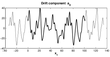
(b) Mean based on 444 configurations, ${\mathcal{T}}=0.8875$

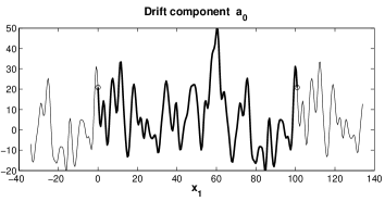
(c) Mean based on 444 configurations, ${\mathcal{T}}=0.2220$

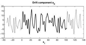
(d) Mean based on 1775 configurations, ${\mathcal{T}}=0.8875$

(e) One single configuration, $X_{{\mbox{}}}^{t}$

(f) Variance based on the configurations in (d)

Figure 15: The term ${\mathcal{A}_{{\mathcal{S}}}\left({a_{0}}\right)}$ is the slowest converging average in the drift average; a comparison with Figure 14 shows that this term dominates the total drift average. This explicit form of the term, given in (18) is a sum over all particles of terms that are second order in the particle forces and a term containing the divergence of the particle force; in the molecular dynamics simulation, these terms are large and so is the function $a_{0}$, when computed from a single configuration, as in (e). Eventually the average must decrease to order 1 through cancellation, but for the number of configurations available here fluctuations dominate the computed averages ${\mathcal{A}_{{\mathcal{S}}}\left({a_{0}}\right)}$.

(a) Mean based on 111 configurations, ${\mathcal{T}}=0.8875$

(b) Mean based on 444 configurations, ${\mathcal{T}}=0.8875$

(c) Mean based on 444 configurations, ${\mathcal{T}}=0.2220$

(d) Mean based on 1775 configurations, ${\mathcal{T}}=0.8875$

Figure 16: The term ${\mathcal{A}_{{\mathcal{S}}}\left({a_{1}}\right)}$ is supposed to approach zero as the number of configurations, and $\mathcal{T}$, increases, provided that the interfaces are stationary. Though the fluctuations are large here, they are much smaller than in Figure 15. When the fluctuations decrease a pattern appears with peaks at the two interfaces. This supports the observation, from the computed ${\mathcal{A}_{{\mathcal{S}}}\left({m}\right)}$ in Figure 8, that the two phase system is not in equilibrium yet and the interfaces are not really stationary on the time scale of the average.

(a) Mean based on 111 configurations, ${\mathcal{T}}=0.8875$

(b) Mean based on 444 configurations, ${\mathcal{T}}=0.8875$

(c) Mean based on 444 configurations, ${\mathcal{T}}=0.2220$

(d) Mean based on 1775 configurations, ${\mathcal{T}}=0.8875$

Figure 17: The average ${k_{\mathrm{B}}}{T}\frac{\partial^{2}}{\partial x_{1}^{2}}{\mathcal{A}_{{\mathcal{S}}}\left({a_{1}}\right)}$ converges faster than the two other terms in ${\mathcal{A}_{{\mathcal{S}}}\left({\alpha}\right)}$. The fluctuations are larger in subfigure (c) than in (b), which indicates that the error is dominated by the length of the averaging time interval rather than the number of configurations sampled within the time interval.

3.2.3 Obtaining the phase-field double-well potential from the drift

When defining a phase-field variable in terms the potential energy in the microscale model in Section 1, the goal was to compute a reaction–diffusion equation, like the Allen-Cahn equation (2b), for the coarse-grained phase-field. In a one dimensional problem, with ${T}\equiv{T_{\mathrm{M}}}$ and $k_{1}$ constant, the Allen-Cahn equation reduces to

$$\frac{\partial{\phi}}{\partial t} =k_{1}\frac{\partial^{2}}{\partial x_{1}^{2}}{\phi}-k_{2}{f}^{\prime}({\phi})+noise,$$ (24)

where the derivative of the double-well potential $f$ gives the reaction part in this reaction–diffusion equation. Now, the coarse-grained equation

$$d{m_{\mathrm{cg}}^{t}}(x_{1}) =\left({k_{\mathrm{B}}}{T}\frac{\partial^{2}}{\partial x_{1}^{2}}{m_{\mathrm{cg}}^{t}}(x_{1})+\frac{\partial}{\partial x_{1}}{\overline{a}}_{1}(x_{1})+{\overline{a}}_{0}(x_{1})\right)dt+{\sum_{j=1}^{M}}{\overline{b}}_{j}(x)\;d{\widetilde{W}}_{j}^{t},$$

where

$${\overline{a}}_{1}(x_{1}) ={\mathcal{A}_{{\mathcal{S}}}\left({a_{1}}\right)}(x_{1}), {\overline{a}}_{0}(x_{1}) ={\mathcal{A}_{{\mathcal{S}}}\left({a_{0}}\right)}(x_{1}) ,\text{for $x_{1}\in D_{K}$,}$$

and the diffusion coefficient vectors, ${\overline{b}}_{j}$, are obtained from the factorisation (20), is a stochastic convection–reaction–diffusion equation. As the described above the time averaged drift is zero in a stationary situation, but in the computations presented here the fluctuations are still too large. In the ideal situation for a stationary interface, when all three components in the drift average have converged, the convection should vanish, that is

$$\frac{\partial}{\partial x_{1}}{\overline{a}}_{1} \equiv 0,$$

and the reaction and diffusion parts should cancel each other, so that

$$0 ={k_{\mathrm{B}}}{T}\frac{\partial^{2}}{\partial x_{1}^{2}}{m_{\mathrm{cg}}^{t}}(x_{1})+{\overline{a}}_{0}(x_{1}).$$ (25)

The second best thing, when some of the computed averages contain too large errors, is to extract information from the most accurate part, that is ${k_{\mathrm{B}}}{T}\frac{\partial^{2}}{\partial x_{1}^{2}}{m}_{\mathrm{av}}(x_{1})$. Assuming that this computed average already is close to what it would be in the ideal situation, an approximation of the reaction term can be obtained from (25).

The expression of the drift in the coarse-grained equation (7) as a function of the coarse-grained phase-field $m_{\mathrm{cg}}$ in the interface regions, instead of the space variable $x_{1}$, assumes monotonicity of the phase-field near the interfaces to allow the inversion in (10). Figure 18 shows ${m}_{\mathrm{av}}(x_{1})$ and ${k_{\mathrm{B}}}{T}\frac{\partial^{2}}{\partial x_{1}^{2}}{m}_{\mathrm{av}}(x_{1})$ in the interval of monotonicity for ${m}_{\mathrm{av}}(x_{1})$ in the simulation O2.

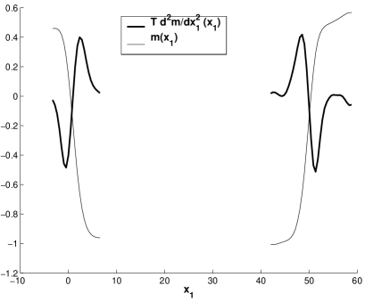
Figure 18: The computed ${m}_{\mathrm{av}}(x_{1})$ in its monotone intervals in the interfaces together with the corresponding diffusion part of the drift ${k_{\mathrm{B}}}{T}\frac{\partial^{2}}{\partial x_{1}^{2}}{\mathcal{A}_{{\mathcal{S}}}\left({a_{1}}\right)}$. The curves shown are part of the those in Figure 8(d) and Figure 17(d).

Using the computed ${k_{\mathrm{B}}}{T}\frac{\partial^{2}}{\partial x_{1}^{2}}{m}_{\mathrm{av}}(x_{1})$ in (25), gives

$${\overline{a}}_{0}(x_{1}) =-{k_{\mathrm{B}}}{T}\frac{\partial^{2}}{\partial x_{1}^{2}}{m}_{\mathrm{av}}(x_{1}).$$

Inverting the computed function ${m}_{\mathrm{av}}(x_{1})$ in the interface intervals, the derivative of the double-well potential $f$ can be identified as

$${f}^{\prime}({m_{\mathrm{cg}}}) ={\overline{a}}_{0}({m}_{\mathrm{av}}^{-1}({m_{\mathrm{cg}}})).$$

Integration with respect to ${m_{\mathrm{cg}}}$ in the interval between ${m_{\mathrm{cg}}}_{\mathrm{solid}}$ and ${m_{\mathrm{cg}}}_{\mathrm{liquid}}$ gives the double-well potentials shown in Figure 19(a). As expected the potentials obtained from the two different simulations O1 and O2 are slightly different. However, the potentials obtained from the two different interfaces in one molecular dynamics simulation cell also differ slightly and it is not possible to say that difference between simulations O1 and O2 depend on the orientation of the interfaces with respect to the crystal lattice. The computed double wells seem to be qualitatively right.

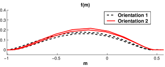
(a) Double well potential, ${\epsilon}=1.0$

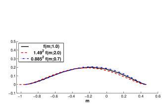
(b) Orientation 2, different $\epsilon$

Figure 19:
(a) The computed double well potentials from both simulation O1 and O2 using ${m}_{\mathrm{av}}$ shown in Figure 8 and the corresponding ${k_{\mathrm{B}}}{T}\frac{\partial^{2}}{\partial x_{1}^{2}}{m}_{\mathrm{av}}(x_{1})$.
(b) The computed double well potentials from one of the interfaces in O2, using three different values of the smoothing parameter $\epsilon$ in the mollifier. Since the interface width varies with $\epsilon$ the height of the potential barriers vary with $\epsilon$. Here double-wells have been rescaled with factors obtained in the analysis of the $\epsilon$-dependence in Figure 27 to compare the shape of the curves.

3.3 The averaged diffusion matrix $\overline{B}$ and the coarse-grained diffusion coefficients ${\overline{b}}_{j}$.

The final component to extract in the coarse-grained model is the diffusion in the stochastic differential equation for $m_{\mathrm{cg}}^{t}$. Using ${\epsilon}=1.0$ and the same 1775 configurations that were used in the computation of the averaged phase-field and drift for simulation O2, the averaged diffusion matrix $\overline{B}$, has been computed, with the result shown in Figure 20(a). As described in Section 2.2, the square root of $\overline{B}$is computed by an eigenvector decomposition where all negative eigenvalues are set to zero; the result is shown in Figure 20(b). The negative eigenvalues are very small in absolute value, compared to the dominating positive ones, so the error made by neglecting them is insignificant when ${B}{{B}^{\mathrm{T}}}$ is compared to $\overline{B}$. By choosing the diffusion coefficients ${\overline{b}}_{j}$ in the coarse-grained stochastic differential equation as the columns of $B$, they become localised in space; see Figure 20(c). With ${\epsilon}=1.0$ the observed difference between the diffusion in the solid part and the liquid part is small, as shown in Figure 21.

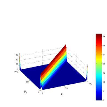
(a) $\overline{B}$

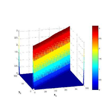
(b) ${B}$

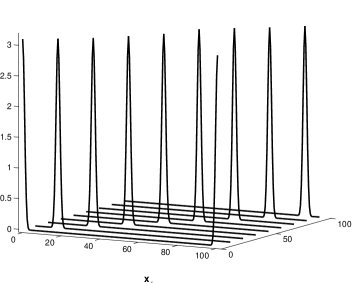
(c) Some ${\overline{b}}_{j}$:s

Figure 20: The computed average diffusion matrix $\overline{B}$, for ${\epsilon}=1.0$, using the same configurations from simulation O2 as in Figure 8(d) and Figure 17(d), is shown in (a). The square root $B$ of $\overline{B}$, as defined in (20) is shown in (b). The individual columns in $B$ are the diffusion coefficient functions, ${\overline{b}}_{j}$, in the stochastic differential equation for the coarse-grained phase-field $m^{t}$. Some of these column vectors have been plotted as functions of the space variable $x_{1}$ in (c). The support of each ${\overline{b}}_{j}$ is centred around the grid point $x_{1}^{j}$.

\begin{picture}(50.0,180.0)(0.0,0.0)\put(0.0,0.0){\makebox(0.0,0.0)[]{}} \end{picture}

(a) FCC, $\epsilon$=2.0

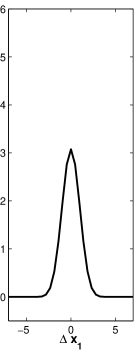
(b) FCC, $\epsilon$=1.0

(c) FCC, $\epsilon$=0.55

\begin{picture}(50.0,180.0)(0.0,0.0)\put(0.0,0.0){\makebox(0.0,0.0)[]{}} \end{picture}

\begin{picture}(50.0,180.0)(0.0,0.0)\put(0.0,0.0){\makebox(0.0,0.0)[]{}} \end{picture}

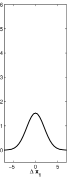
(d) Liquid, $\epsilon$=2.0

(e) Liquid, $\epsilon$=1.0

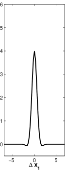
(f) Liquid, $\epsilon$=0.55

\begin{picture}(50.0,180.0)(0.0,0.0)\put(0.0,0.0){\makebox(0.0,0.0)[]{}} \end{picture}

Figure 21: The average diffusion coefficient functions, $\tilde{{\overline{b}}}(\Delta x_{1})=\mathrm{mean}\left\{{\overline{b}}_{j}(x_{1}^{j}+\Delta x_{1})\right\}$ have been computed for different values of $\epsilon$, with the mean taken over points $x_{1}^{j}$ in the interior of the solid and the liquid domains, respectively. The configurations used are the same as in Figure 20. The difference between the solid and liquid parts is small.

3.4 Dependence on the smoothing parameter

The mollifier $\eta$ includes a parameter, $\epsilon$, determining the scale on which the local average is taken. This is in itself an ad hoc variable in the micro model and it is important to analyse its effects on the computed quantities.

A lower limit on $\epsilon$ is set by the demand that the phase-field be approximately constant in the solid in spite of the periodic structure. If the solid structure is aligned with the computational domain in such a way that the global spatial averages are taken parallel to atomic layers, then the parameter $\epsilon$ controlling the width of the average in the orthogonal direction must be large enough to smooth the gaps between the atomic layers. In the numerical simulations the orientations of the FCC lattice with respect to the solid–liquid interface, and hence the planes of averaging, are precisely such that averages are computed parallel to atomic planes, as illustrated in Figure 22.

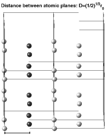
(a) Orientation 1

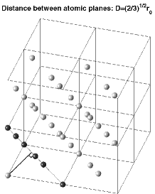
(b) Orientation 2

Figure 22: The distance between two adjacent atom layers in a perfect FCC lattice is $\sqrt{1/2}\,r_{0}$ in orientation 1 and $\sqrt{2/3}\,r_{0}$ in orientation 2, where $r_{0}$ is the nearest neighbour distance.

In the present case the distance to the nearest neighbours in the FCC-lattice is around 1.02; with $\eta$ on the form (16) the parameter $\epsilon$ must be taken greater than $0.43$ to ensure that $\eta$ decreases with at most a factor $1/2$ in half the distance to the nearest neighbour, which seems a reasonable demand. Figure 23, presenting computed phase-fields based on local averages of the density and the potential energy using ${\epsilon}=0.45$, shows that the smoothing parameter has to be larger than this to avoid oscillations in the solid part. The phase-fields based on ${\epsilon}=0.70$ in Figure 24 do not show these oscillations on the length scale smaller than the distance between atom layers.

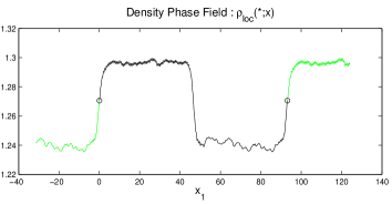
(a) Orientation 1

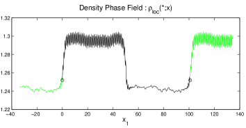
(b) Orientation 2

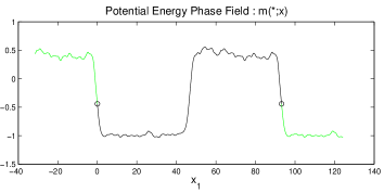
(c) Orientation 1

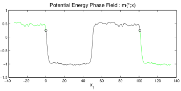
(d) Orientation 2

Figure 23: Computed density, ${\rho}_{loc}$, and potential energy phase fields for simulations O1 and O2 using ${\epsilon}=0.45$.

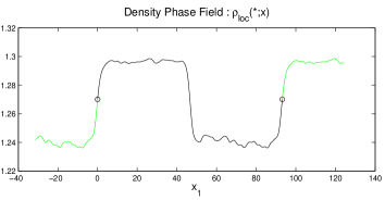
(a) Orientation 1

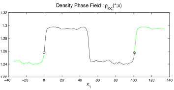
(b) Orientation 2

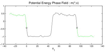
(c) Orientation 1

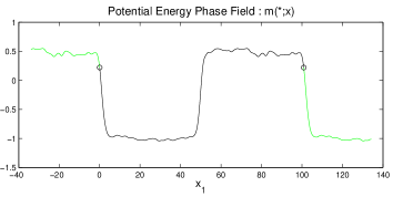
(d) Orientation 2

Figure 24: Computed density, ${\rho}_{loc}$, and potential energy phase fields for simulations O1 and O2 using ${\epsilon}=0.70$.

For the method to be reasonable, the lower bound on $\epsilon$ must not hide an interface width in the phase-field that is sharp even on the atomic scale. In addition to the computations with ${\epsilon}=1.0$, the phase field has been computed for ${\epsilon}=0.45,\,0.70,\,\mbox{and}\,2.0$. The computed phase-fields in the regions around the interfaces, for both orientation 1 and 2, are shown in Figure 25. The comparison shows that the interface width varies with the smoothing parameter. It would not, however, become infinitely sharp in the limit when $\epsilon$ goes to zero, even if the lower bound on $\epsilon$ were disregarded. This is clear from the results presented in Figure 26 where, in addition to the values of $\epsilon$ above, a phase-field obtained with ${\epsilon}=0.05$, violating the lower bound, is shown around one of the interfaces in O1. This value of the smoothing parameter, and the corresponding mollifier cutoff, $R_{c}=6\cdot 0.05=0.3$, is so small that the contribution to the phase-field of an individual atom in the FCC lattice is restricted to an interval extending less than half way to the next atom layer in either direction. Still the change in the phase-field, from strong oscillations in the solid to decaying oscillations around the average in the pure liquid, occurs gradually on a length scale corresponding to at least several atom layers and thus several times the artificial smoothing introduced by $\epsilon$. Figure 26 also shows that the interface region of the phase-field obtained with ${\epsilon}=0.45,\,0.70,\,\mbox{and}\,1.0$ is wider than the transition region of a step function, representing an infinitely sharp interface, smoothed by a convolution with the mollifier using the corresponding $\epsilon$. For ${\epsilon}=2.0$ the interface is very close to that of a mollified step function in both width and profile. The interface width of the smoothed step function is proportional to $\epsilon$ and it is expected that the same will hold for the phase-field, $m$, if the smoothing parameter is increased beyond the present range.

\begin{picture}(100.0,120.0)(0.0,0.0)\put(0.0,0.0){\makebox(0.0,0.0)[]{}} \end{picture}

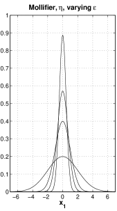
(a) Mollifier, $\eta$

\begin{picture}(100.0,120.0)(0.0,0.0)\put(0.0,0.0){\makebox(0.0,0.0)[]{}} \end{picture}

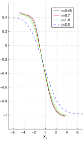
(b) Orientation 1

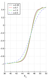
(c) Orientation 1

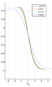
(d) Orientation 2

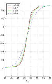
(e) Orientation 2

Figure 25: The mollifier, ${\eta}$, in the definition of the phase field, $m$, depends on the model parameter $\epsilon$. The width of the averaging is proportional to $\epsilon$, as illustrated in (a) which shows $\eta$ for ${\epsilon}=0.45,\,0.7,\,1.0,\,2.0$.
The phase field, $m$, in the interface regions has been computed from 174 configurations with the four $\epsilon$-values listed above. In (b) and (c) the configurations are taken from simulation O1, and in (d) and (e) from simulation O2. In each case the time interval between two successive configurations is $2.5\cdot 10^{-3}$, corresponding to $5\cdot 10^{3}$ time steps. Though the interface width in the computed phase-fields varies with $\epsilon$, it is not proportional to $\epsilon$ in this range.

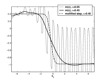
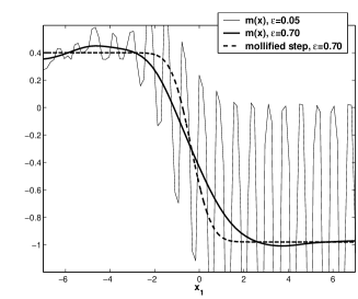
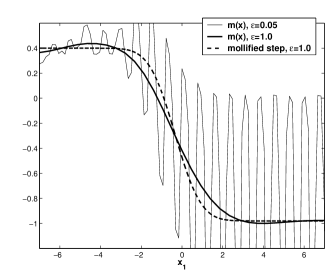
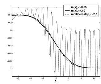
Figure 26: For the phase field based on local contributions to the potential energy the transition from solid to liquid occurs on a length scale of at least several nearest neighbour distances for any choice of the smoothing parameter $\epsilon$.
The four subfigures are based on the same configurations from simulation O1 as were Figure 25(b)–25(c). The oscillating curve present in all subfigures is the computed phase-field, $m$, using ${\epsilon}=0.05$ with a cutoff of $\eta$ at $0.3$. The nearest neighbour distance is approximately 1 and, for the present orientation of the FCC structure with respect to the $x_{1}$-axis, the $x_{1}$-distance between the atomic layers becomes approximately $1/\sqrt{2}$. Since the cutoff is less than half the distance between the atomic layers the phase-field would be exactly zero at the middle distance if the crystal were perfect and it is very close to zero here. The transition from the stable oscillation pattern in the solid to diminishing oscillations around the mean in the liquid is extended over a distance corresponding to at least four or five atomic layers in the solid.
The phase-field, $m$, for ${\epsilon}=0.45,\,0.70,\,1.0,\,\mathrm{and}\,2.0$ is shown as the heavy solid curve in subfigures (a)–(d). For reference the convolutions $\int_{-\infty}^{\infty}f(y){\eta}(x-y)\;dy$ of a sharp interface, given by the step function $f(y)=m_{\mathrm{liq}}{\mathbf{1}_{{\mathbb{R}^{-}}}}(y)-m_{\mathrm{FCC}}{\mathbf{1}_{{\mathbb{R}^{+}}}}(y)$, and the mollifier using the respective $\epsilon$-value is included as the heavy dashed curve. For the smaller $\epsilon$-values the mollified step function is significantly sharper than the corresponding phase-field.

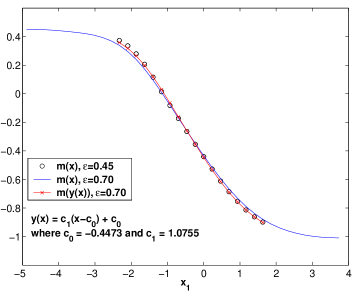
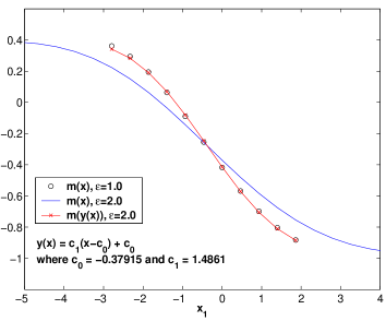
		approximating $\epsilon$
		0.70	1.0	2.0
	0.45	1.09 (1.56)	1.23 (2.22)	1.82 (4.44)
reference $\epsilon$	0.70		1.13 (1.43)	1.68 (2.86)
	1.0			1.49 (2.00)

(a) Rescaling factors – the accuracy is approximately $\pm 0.05$.

Figure 27: For an interface given by the convolution of a sharp step function and the mollifier, as in Figure 26, the interface width is directly proportional to $\epsilon$, since interface profiles corresponding to different $\epsilon$ are identical up to affine coordinate transformations around the interface, $x_{\mathrm{if}}$, that is: ${\phi}_{{\epsilon}_{2}}(\frac{{\epsilon}_{2}}{{\epsilon}_{1}}(x-x_{\mathrm{if}})+x_{\mathrm{if}})={\phi}_{{\epsilon}_{1}}(x)$. On a sufficiently large scale the same scaling of the interface width can be expected from the phase-field $m$ obtained from MD simulations. This is not the case when $\epsilon$ is of the order of the nearest neighbour distance; then the interface width grows more slowly than $\epsilon$. One way to quantify this statement is to consider the tabulated phase-field, ${m}_{{\epsilon}_{1}}$, using the parameter value ${\epsilon}_{1}$, as given data to be approximated by the phase-field, ${m}_{{\epsilon}_{2}}$, based on the parameter value ${\epsilon}_{2}$; the allowed approximations use affine coordinate transformations $y(x)=c_{1}(x-c_{0})+c_{0}$ of the independent coordinate. The data points $((x_{k}),{m}_{{\epsilon}_{1}}(x_{k}))$ are taken from the interior of an interface, ${m}_{\mathrm{solid}}<m_{0}\leq{m}_{{\epsilon}_{1}}(x_{k})\leq m_{1}<{m}_{\mathrm{liquid}}$, and the function ${m}_{{\epsilon}_{2}}$ is defined by linear interpolation between tabulated values. A least squares approximation of the overdetermined system ${m}_{{\epsilon}_{2}}(y(x_{k}))={m}_{{\epsilon}_{1}}(x_{k})$ for $c_{0}$ and $c_{1}$ gives a value of the scaling factor $c_{1}$ to be compared to ${\epsilon}_{2}/{\epsilon}_{1}$.
Subfigures (a) and (b) show two examples for the interface in Figure 25(b). The circles, $\circ$, denote the reference data points, the solid line shows the linear interpolation of the tabulated values for the approximating phase-field, and the line marked with crosses, $\times$, is the least square approximation.
The table (c) shows the scaling constants obtained after averaging over all four interfaces in Figure 25(b)–25(e). The corresponding quotients $\frac{{\epsilon}_{2}}{{\epsilon}_{1}}$ are included in parenthesis for reference.

Appendix A Explicit Calculation of Drift and Diffusion Functions

Let the total potential energy be

$${U}({X_{{\mbox{}}}^{t}}) ={\sum_{i=1}^{N}}{m_{i}}({{X_{{\mbox{}}}^{{\mbox{}}}}}),$$

where

$${m_{i}}({{X_{{\mbox{}}}^{{\mbox{}}}}}) =\frac{1}{2}{\sum_{k\neq i,k=1}^{N}}{\Phi}(||{X_{i}^{{\mbox{}}}}-{X_{k}^{{\mbox{}}}}||).$$

For the phase-field

$${m}(x;{{X_{{\mbox{}}}^{{\mbox{}}}}}) ={\sum_{i=1}^{N}}{m_{i}}({{X_{{\mbox{}}}^{{\mbox{}}}}}){\eta}(x-{X_{i}^{{\mbox{}}}}),$$

where the particle positions $${{X_{{\mbox{}}}^{{\mbox{}}}}}\in\mathbb{R}^{3{N}}$$ solve the Itô stochastic differential equation

$$d{X_{{\mbox{}}}^{t}} =-\nabla_{{{X_{{\mbox{}}}^{{\mbox{}}}}}}{U}({X_{{\mbox{}}}^{t}})\;dt+\sqrt{2{k_{\mathrm{B}}}{T}}\;dW^{t},$$

Itô’s formula gives

$$d{m}(x;{X_{{\mbox{}}}^{t}}) ={\sum_{j=1}^{N}}{\alpha}_{j}(x;{X_{{\mbox{}}}^{t}})\,dt+{\sum_{j=1}^{N}}\sum_{k=1}^{3}{\beta}_{j,k}(x;{X_{{\mbox{}}}^{t}})\,dW_{j,k}^{t},$$

with

$${\alpha}_{j}(x;{{X_{{\mbox{}}}^{{\mbox{}}}}}) =-\nabla_{X_{j}}{m}(x;{{X_{{\mbox{}}}^{{\mbox{}}}}})\cdot\nabla_{X_{j}}{U}({{X_{{\mbox{}}}^{{\mbox{}}}}})+{k_{\mathrm{B}}}{T}\nabla_{X_{j}}\!\cdot\!\nabla_{X_{j}}{m}(x;{{X_{{\mbox{}}}^{{\mbox{}}}}})$$ (26)

and

$${\beta}_{j,\cdot}(x;{{X_{{\mbox{}}}^{{\mbox{}}}}}) =\sqrt{2{k_{\mathrm{B}}}{T}}\nabla_{X_{j}}{m}(x;{{X_{{\mbox{}}}^{{\mbox{}}}}}).$$ (27)

Introducing the total force, $${F}_{j} j {f}_{ij}$$, acting on particle , and the contributions from individual pairs, ,

$${F}_{j}({{X_{{\mbox{}}}^{{\mbox{}}}}}) =-\nabla_{X_{j}}{U}({{X_{{\mbox{}}}^{{\mbox{}}}}})={\sum_{i\neq j,i=1}^{N}}{f}_{ij}({{X_{{\mbox{}}}^{{\mbox{}}}}}),$$

$${f}_{ij}({{X_{{\mbox{}}}^{{\mbox{}}}}}) ={\Phi}^{\prime}(||{X_{i}^{{\mbox{}}}}-{X_{j}^{{\mbox{}}}}||)\frac{{X_{i}^{{\mbox{}}}}-{X_{j}^{{\mbox{}}}}}{||{X_{i}^{{\mbox{}}}}-{X_{j}^{{\mbox{}}}}||},$$

the gradient of ${m_{i}}$ with respect to the position of particle $j$ is

$$\nabla_{X_{j}}{m_{i}}({{X_{{\mbox{}}}^{{\mbox{}}}}}) =\frac{1}{2}{\sum_{k\neq i,k=1}^{N}}\nabla_{X_{j}}{\Phi}(||{X_{i}^{{\mbox{}}}}-{X_{k}^{{\mbox{}}}}||)$$

$$=\delta_{ij}\frac{1}{2}{\sum_{k\neq j,k=1}^{N}}\nabla_{X_{j}}{\Phi}(||{X_{j}^{{\mbox{}}}}-{X_{k}^{{\mbox{}}}}||)+(1-\delta_{ij})\frac{1}{2}\nabla_{X_{j}}{\Phi}(||{X_{i}^{{\mbox{}}}}-{X_{j}^{{\mbox{}}}}||)$$

$$=-\delta_{ij}\frac{1}{2}{F}_{j}({{X_{{\mbox{}}}^{{\mbox{}}}}})-(1-\delta_{ij})\frac{1}{2}{f}_{ij}({{X_{{\mbox{}}}^{{\mbox{}}}}}),$$

where $\delta_{ij}$ is the Kronecker delta: $\delta_{ij}=1,\text{if $i=j$},\delta_{ij}=0,\text{if $i\neq j$}$. The gradient of the phase-field variable with respect to the position of particle $j$ is

$$\nabla_{X_{j}}{m}(x;{{X_{{\mbox{}}}^{{\mbox{}}}}}) ={m_{j}}({{X_{{\mbox{}}}^{{\mbox{}}}}})\nabla_{X_{j}}{\eta}(x-{X_{j}^{{\mbox{}}}})+{\sum_{i=1}^{N}}\nabla_{X_{j}}{m_{i}}({{X_{{\mbox{}}}^{{\mbox{}}}}}){\eta}(x-{X_{i}^{{\mbox{}}}})$$

$$=-{m_{j}}({{X_{{\mbox{}}}^{{\mbox{}}}}})\nabla_{x}{\eta}(x-{X_{j}^{{\mbox{}}}})$$

$$\quad-\frac{1}{2}{\sum_{i=1}^{N}}\delta_{ij}{F}_{j}({{X_{{\mbox{}}}^{{\mbox{}}}}}){\eta}(x-{X_{i}^{{\mbox{}}}})-\frac{1}{2}{\sum_{i=1}^{N}}(1-\delta_{ij}){f}_{ij}({{X_{{\mbox{}}}^{{\mbox{}}}}}){\eta}(x-{X_{i}^{{\mbox{}}}})$$

$$=-\nabla_{x}({m_{j}}({{X_{{\mbox{}}}^{{\mbox{}}}}}){\eta}(x-{X_{j}^{{\mbox{}}}}))$$

$$\quad-\frac{1}{2}{F}_{j}({{X_{{\mbox{}}}^{{\mbox{}}}}}){\eta}(x-{X_{j}^{{\mbox{}}}})-\frac{1}{2}{\sum_{i\neq j,i=1}^{N}}{f}_{ij}({{X_{{\mbox{}}}^{{\mbox{}}}}}){\eta}(x-{X_{i}^{{\mbox{}}}}).$$

Introducing the notation $-{G}_{j}$ for the divergence of the force ${F}_{j}$ with respect to ${X_{j}^{{\mbox{}}}}$ and the notation ${g}_{ij}$ for the individual contributions,

$${G}_{j}({{X_{{\mbox{}}}^{{\mbox{}}}}}) =-\nabla_{X_{j}}\cdot{F}_{j}({{X_{{\mbox{}}}^{{\mbox{}}}}})=-{\sum_{i\neq j,i=1}^{N}}\nabla_{X_{j}}\cdot{f}_{ij}({{X_{{\mbox{}}}^{{\mbox{}}}}})={\sum_{i\neq j,i=1}^{N}}{g}_{ij}({{X_{{\mbox{}}}^{{\mbox{}}}}}),$$

$${g}_{ij}({{X_{{\mbox{}}}^{{\mbox{}}}}}) ={\Phi}^{\prime\prime}(||{X_{i}^{{\mbox{}}}}-{X_{j}^{{\mbox{}}}}||)+{\Phi}^{\prime}(||{X_{i}^{{\mbox{}}}}-{X_{j}^{{\mbox{}}}}||)\frac{2}{||{X_{i}^{{\mbox{}}}}-{X_{j}^{{\mbox{}}}}||},$$

the divergence of gradient of phase field variable with respect to the position of particle $j$ becomes

$$\nabla_{X_{j}}\!\cdot\!\nabla_{X_{j}}{m}(x;{{X_{{\mbox{}}}^{{\mbox{}}}}}) =-\nabla_{X_{j}}\cdot\left({m_{j}}({{X_{{\mbox{}}}^{{\mbox{}}}}})\nabla_{x}{\eta}(x-{X_{j}^{{\mbox{}}}})\right)$$

$$\quad-\frac{1}{2}\nabla_{X_{j}}\cdot\left({F}_{j}({{X_{{\mbox{}}}^{{\mbox{}}}}}){\eta}(x-{X_{j}^{{\mbox{}}}})\right)-\frac{1}{2}{\sum_{i\neq j,i=1}^{N}}\nabla_{X_{j}}\cdot\left({f}_{ij}({{X_{{\mbox{}}}^{{\mbox{}}}}}){\eta}(x-{X_{i}^{{\mbox{}}}})\right)$$

$$=-\nabla_{X_{j}}{m_{j}}({{X_{{\mbox{}}}^{{\mbox{}}}}})\cdot\nabla_{x}{\eta}(x-{X_{j}^{{\mbox{}}}})-{m_{j}}({{X_{{\mbox{}}}^{{\mbox{}}}}})\nabla_{X_{j}}\cdot\nabla_{x}{\eta}(x-{X_{j}^{{\mbox{}}}})$$

$$\quad-\frac{1}{2}\nabla_{X_{j}}\cdot{F}_{j}({{X_{{\mbox{}}}^{{\mbox{}}}}}){\eta}(x-{X_{j}^{{\mbox{}}}})-\frac{1}{2}{F}_{j}({{X_{{\mbox{}}}^{{\mbox{}}}}})\cdot\nabla_{X_{j}}{\eta}(x-{X_{j}^{{\mbox{}}}})$$

$$\quad-\frac{1}{2}{\sum_{i\neq j,i=1}^{N}}\nabla_{X_{j}}\cdot{f}_{ij}({{X_{{\mbox{}}}^{{\mbox{}}}}}){\eta}(x-{X_{i}^{{\mbox{}}}})$$

$$=\frac{1}{2}{F}_{j}({{X_{{\mbox{}}}^{{\mbox{}}}}})\cdot\nabla_{x}{\eta}(x-{X_{j}^{{\mbox{}}}})+{m_{j}}({{X_{{\mbox{}}}^{{\mbox{}}}}})\nabla_{x}\cdot\nabla_{x}{\eta}(x-{X_{j}^{{\mbox{}}}})$$

$$\quad+\frac{1}{2}{G}_{j}({{X_{{\mbox{}}}^{{\mbox{}}}}}){\eta}(x-{X_{j}^{{\mbox{}}}})+\frac{1}{2}{F}_{j}({{X_{{\mbox{}}}^{{\mbox{}}}}})\cdot\nabla_{x}{\eta}(x-{X_{j}^{{\mbox{}}}})$$

$$\quad+\frac{1}{2}{\sum_{i\neq j,i=1}^{N}}{g}_{ij}({{X_{{\mbox{}}}^{{\mbox{}}}}}){\eta}(x-{X_{i}^{{\mbox{}}}})$$

$$=\nabla_{x}\!\cdot\!\nabla_{x}\left({m_{j}}({{X_{{\mbox{}}}^{{\mbox{}}}}}){\eta}(x-{X_{j}^{{\mbox{}}}})\right)+\nabla_{x}\cdot\left({F}_{j}({{X_{{\mbox{}}}^{{\mbox{}}}}}){\eta}(x-{X_{j}^{{\mbox{}}}})\right)$$

$$\quad+\frac{1}{2}{G}_{j}({{X_{{\mbox{}}}^{{\mbox{}}}}}){\eta}(x-{X_{j}^{{\mbox{}}}})+\frac{1}{2}{\sum_{i\neq j,i=1}^{N}}{g}_{ij}({{X_{{\mbox{}}}^{{\mbox{}}}}}){\eta}(x-{X_{i}^{{\mbox{}}}}).$$

Using the explicit expressions for $\nabla_{X_{j}}{m}(x;{{X_{{\mbox{}}}^{{\mbox{}}}}})$ and $\nabla_{X_{j}}\!\cdot\!\nabla_{X_{j}}{m}(x;{{X_{{\mbox{}}}^{{\mbox{}}}}})$, the components (26) of the drift become

$${\alpha}_{j}(x;{{X_{{\mbox{}}}^{{\mbox{}}}}}) =\nabla_{x}({m_{j}}({{X_{{\mbox{}}}^{{\mbox{}}}}}){\eta}(x-{X_{j}^{{\mbox{}}}}))\cdot(-{F}_{j}({{X_{{\mbox{}}}^{{\mbox{}}}}}))+\frac{1}{2}{F}_{j}({{X_{{\mbox{}}}^{{\mbox{}}}}}){\eta}(x-{X_{j}^{{\mbox{}}}})\cdot(-{F}_{j}({{X_{{\mbox{}}}^{{\mbox{}}}}}))$$

$$\quad+\frac{1}{2}{\sum_{i\neq j,i=1}^{N}}{f}_{ij}({{X_{{\mbox{}}}^{{\mbox{}}}}}){\eta}(x-{X_{i}^{{\mbox{}}}})\cdot(-{F}_{j}({{X_{{\mbox{}}}^{{\mbox{}}}}}))$$

$$\quad+{k_{\mathrm{B}}}{T}\nabla_{X_{j}}\!\cdot\!\nabla_{X_{j}}{m}(x;{{X_{{\mbox{}}}^{{\mbox{}}}}})$$

$$=-\nabla_{x}\cdot({m_{j}}({{X_{{\mbox{}}}^{{\mbox{}}}}}){F}_{j}({{X_{{\mbox{}}}^{{\mbox{}}}}}){\eta}(x-{X_{j}^{{\mbox{}}}}))-\frac{1}{2}||{F}_{j}({{X_{{\mbox{}}}^{{\mbox{}}}}})||^{2}{\eta}(x-{X_{j}^{{\mbox{}}}})$$

$$\quad-\frac{1}{2}{\sum_{i\neq j,i=1}^{N}}{f}_{ij}({{X_{{\mbox{}}}^{{\mbox{}}}}})\cdot{F}_{j}({{X_{{\mbox{}}}^{{\mbox{}}}}}){\eta}(x-{X_{i}^{{\mbox{}}}})$$

$$\quad+{k_{\mathrm{B}}}{T}\nabla_{x}\!\cdot\!\nabla_{x}\left({m_{j}}({{X_{{\mbox{}}}^{{\mbox{}}}}}){\eta}(x-{X_{j}^{{\mbox{}}}})\right)+{k_{\mathrm{B}}}{T}\nabla_{x}\cdot\left({F}_{j}({{X_{{\mbox{}}}^{{\mbox{}}}}}){\eta}(x-{X_{j}^{{\mbox{}}}})\right)$$

$$\quad+{k_{\mathrm{B}}}{T}\frac{1}{2}{G}_{j}({{X_{{\mbox{}}}^{{\mbox{}}}}}){\eta}(x-{X_{j}^{{\mbox{}}}})+{k_{\mathrm{B}}}{T}\frac{1}{2}{\sum_{i\neq j,i=1}^{N}}{g}_{ij}({{X_{{\mbox{}}}^{{\mbox{}}}}}){\eta}(x-{X_{i}^{{\mbox{}}}}).$$

$$={k_{\mathrm{B}}}{T}\nabla_{x}\!\cdot\!\nabla_{x}\bigl{(}{m_{j}}({{X_{{\mbox{}}}^{{\mbox{}}}}}){\eta}(x-{X_{j}^{{\mbox{}}}})\bigr{)}$$

$$\quad+\nabla_{x}\cdot\biggl{(}({k_{\mathrm{B}}}{T}-{m_{j}}({{X_{{\mbox{}}}^{{\mbox{}}}}})){F}_{j}({{X_{{\mbox{}}}^{{\mbox{}}}}}){\eta}(x-{X_{j}^{{\mbox{}}}})\biggr{)}$$

$$\quad+\frac{1}{2}\bigl{(}{k_{\mathrm{B}}}{T}{G}_{j}({{X_{{\mbox{}}}^{{\mbox{}}}}})-||{F}_{j}({{X_{{\mbox{}}}^{{\mbox{}}}}})||^{2}\bigr{)}{\eta}(x-{X_{j}^{{\mbox{}}}})$$

$$\quad+\frac{1}{2}{\sum_{i\neq j,i=1}^{N}}\bigl{(}{k_{\mathrm{B}}}{T}{g}_{ij}({{X_{{\mbox{}}}^{{\mbox{}}}}})-{f}_{ij}({{X_{{\mbox{}}}^{{\mbox{}}}}})\cdot{F}_{j}({{X_{{\mbox{}}}^{{\mbox{}}}}})\bigr{)}{\eta}(x-{X_{i}^{{\mbox{}}}})$$

so that, after summing over $j$,

$${\alpha}(x;{{X_{{\mbox{}}}^{{\mbox{}}}}}) ={k_{\mathrm{B}}}{T}\nabla_{x}\!\cdot\!\nabla_{x}{m}(x;{{X_{{\mbox{}}}^{{\mbox{}}}}})+\nabla_{x}\cdot\widetilde{a_{1}}(x;{{X_{{\mbox{}}}^{{\mbox{}}}}})+{a_{0}}(x;{{X_{{\mbox{}}}^{{\mbox{}}}}})$$

with

$$\widetilde{a_{1}}(x;{{X_{{\mbox{}}}^{{\mbox{}}}}}) ={\sum_{j=1}^{N}}({k_{\mathrm{B}}}{T}-{m_{j}}({{X_{{\mbox{}}}^{{\mbox{}}}}})){F}_{j}({{X_{{\mbox{}}}^{{\mbox{}}}}}){\eta}(x-{X_{j}^{{\mbox{}}}})$$

and

$${a_{0}}(x;{{X_{{\mbox{}}}^{{\mbox{}}}}}) ={\sum_{j=1}^{N}}\left({k_{\mathrm{B}}}{T}{G}_{j}({{X_{{\mbox{}}}^{{\mbox{}}}}})-\frac{1}{2}||{F}_{j}({{X_{{\mbox{}}}^{{\mbox{}}}}})||^{2}\right){\eta}(x-{X_{j}^{{\mbox{}}}})$$

$$\quad-\frac{1}{2}{\sum_{j=1}^{N}}{\sum_{i\neq j,i=1}^{N}}{f}_{ij}({{X_{{\mbox{}}}^{{\mbox{}}}}})\cdot{F}_{j}({{X_{{\mbox{}}}^{{\mbox{}}}}}){\eta}(x-{X_{i}^{{\mbox{}}}}).$$

Using the one-dimensional mollifier

$${\eta}(x) ={\eta}(x_{1})=\text{constant}\cdot\exp{\left(-\frac{1}{2}\left(\frac{x_{1}}{\epsilon}\right)^{2}\right)},$$ (28)

that only varies in the $x_{1}$-direction, the expression for the drift reduces to

$${\alpha}(x;{{X_{{\mbox{}}}^{{\mbox{}}}}}) ={k_{\mathrm{B}}}{T}\frac{\partial^{2}}{\partial x_{1}^{2}}{m}(x;{{X_{{\mbox{}}}^{{\mbox{}}}}})+\frac{\partial}{\partial x_{1}}{a_{1}}(x;{{X_{{\mbox{}}}^{{\mbox{}}}}})+{a_{0}}(x;{{X_{{\mbox{}}}^{{\mbox{}}}}})$$

with

$${a_{1}}(x;{{X_{{\mbox{}}}^{{\mbox{}}}}}) ={\sum_{j=1}^{N}}({k_{\mathrm{B}}}{T}-{m_{j}}({{X_{{\mbox{}}}^{{\mbox{}}}}}))[{F}_{j}({{X_{{\mbox{}}}^{{\mbox{}}}}})]_{1}{\eta}(x-{X_{j}^{{\mbox{}}}}),$$

where $[{F}_{j}({{X_{{\mbox{}}}^{{\mbox{}}}}})]_{1}$ is the $x_{1}$ component of ${F}_{j}({{X_{{\mbox{}}}^{{\mbox{}}}}})$.

For the purpose of computing an approximation of

$$\frac{1}{{\mathcal{T}}}{\mathrm{E}}\left[\int_{1}^{\mathcal{T}}{\sum_{j=1}^{N}}\sum_{k=1}^{3}{\beta}_{j,k}\otimes{\beta}_{j,k}\right]$$

it is not practical to postpone the differentiation of the mollifier with respect to the space varible. Using the choice (28), the gradient of the mollifier can be expressed in terms of the mollifier itself as

$$\nabla_{x}{\eta}(x-{X_{j}^{{\mbox{}}}}) =\frac{-1}{\epsilon^{2}}{\eta}(x-{X_{j}^{{\mbox{}}}})\left(\left[x-{X_{j}^{{\mbox{}}}}\right]_{1},0,0\right)^{T}.$$

Then the expression for $\nabla_{X_{j}}{m}(x;{{X_{{\mbox{}}}^{{\mbox{}}}}})$ becomes

$$\nabla_{X_{j}}{m}(x;{{X_{{\mbox{}}}^{{\mbox{}}}}}) =\left(\frac{{m_{j}}({{X_{{\mbox{}}}^{{\mbox{}}}}})}{\epsilon^{2}}\left(\left[x-{X_{j}^{{\mbox{}}}}\right]_{1},0,0\right)^{T}-\frac{1}{2}{F}_{j}({{X_{{\mbox{}}}^{{\mbox{}}}}})\right){\eta}(x-{X_{j}^{{\mbox{}}}})$$

$$\quad-\frac{1}{2}{\sum_{i\neq j,i=1}^{N}}{f}_{ij}({{X_{{\mbox{}}}^{{\mbox{}}}}}){\eta}(x-{X_{i}^{{\mbox{}}}})$$

and, using the diffusion component (27),

$$\sum_{k=1}^{3}{\beta}_{j,k}(x;{{X_{{\mbox{}}}^{{\mbox{}}}}}){\beta}_{j,k}(y;{{X_{{\mbox{}}}^{{\mbox{}}}}}) =2{k_{\mathrm{B}}}{T}\biggl{(}p_{j}(x,y;{{X_{{\mbox{}}}^{{\mbox{}}}}})+q_{j}(x,y;{{X_{{\mbox{}}}^{{\mbox{}}}}})\biggr{)},$$

where

$$p_{j}(x,y;{{X_{{\mbox{}}}^{{\mbox{}}}}}) =\left(\frac{{m_{j}}({{X_{{\mbox{}}}^{{\mbox{}}}}})}{\epsilon^{2}}\right)^{2}\left[x-{X_{j}^{{\mbox{}}}}\right]_{1}\left[y-{X_{j}^{{\mbox{}}}}\right]_{1}{\eta}(x-{X_{j}^{{\mbox{}}}}){\eta}(y-{X_{j}^{{\mbox{}}}})$$

$$\quad-\frac{{m_{j}}({{X_{{\mbox{}}}^{{\mbox{}}}}})}{2\epsilon^{2}}[x-{X_{j}^{{\mbox{}}}}]_{1}{\eta}(x-{X_{j}^{{\mbox{}}}})\biggl{(}[{F}_{j}({{X_{{\mbox{}}}^{{\mbox{}}}}})]_{1}{\eta}(y-{X_{j}^{{\mbox{}}}})+\!\!{\sum_{i\neq j,i=1}^{N}}[{f}_{ij}({{X_{{\mbox{}}}^{{\mbox{}}}}})]_{1}{\eta}(y-{X_{i}^{{\mbox{}}}})\biggr{)}$$

$$\quad-\frac{{m_{j}}({{X_{{\mbox{}}}^{{\mbox{}}}}})}{2\epsilon^{2}}[y-{X_{j}^{{\mbox{}}}}]_{1}{\eta}(y-{X_{j}^{{\mbox{}}}})\biggl{(}[{F}_{j}({{X_{{\mbox{}}}^{{\mbox{}}}}})]_{1}{\eta}(x-{X_{j}^{{\mbox{}}}})+\!\!{\sum_{i\neq j,i=1}^{N}}[{f}_{ij}({{X_{{\mbox{}}}^{{\mbox{}}}}})]_{1}{\eta}(x-{X_{i}^{{\mbox{}}}})\biggr{)}$$

and

$$q_{j}(x,y;{{X_{{\mbox{}}}^{{\mbox{}}}}}) =\frac{1}{4}\biggl{(}{F}_{j}({{X_{{\mbox{}}}^{{\mbox{}}}}}){\eta}(x-{X_{j}^{{\mbox{}}}})+{\sum_{i\neq j,i=1}^{N}}{f}_{ij}({{X_{{\mbox{}}}^{{\mbox{}}}}}){\eta}(x-{X_{i}^{{\mbox{}}}})\biggr{)}$$

$$\quad\quad\cdot\biggl{(}{F}_{j}({{X_{{\mbox{}}}^{{\mbox{}}}}}){\eta}(y-{X_{j}^{{\mbox{}}}})+{\sum_{i\neq j,i=1}^{N}}{f}_{ij}({{X_{{\mbox{}}}^{{\mbox{}}}}}){\eta}(y-{X_{i}^{{\mbox{}}}})\biggr{)}.$$

References

- [1] A. B. Belonoshko, O. LeBacq, R. Ahuja, and B. Johansson, Molecular dynamics study of phase transitions in Xe, J. Chem. Phys. 117 (2002), no. 15, 7233–7244.
- [2] W. J. Boettinger, J. A. Warren, C. Beckermann, and A. Karma, Phase-Field Simulation of Solidification, Annu. Rev. Mater. Res. 32 (2002), 163–194.
- [3] E. Cancès, F. Legoll, and G. Stoltz, Theoretical and Numerical Comparison of Some Sampling Methods for Molecular Dynamics, Preprint IMA 2040 (2005).
- [4] M. Dzugutov, mik@pdc.kth.se
- [5] A. J. Majda and P. R. Kramer, Stochastic Mode Reduction for Particle-Based Simulation Methods for Complex Microfluid Systems, SIAM Journal on Applied Mathematics, 64 (2004), no. 2, 401–422.
- [6] G. Marsaglia and W. W. Tsang, The ziggurat method for generating random variables, J. Statist. Software, 5 (2000), no. 8, 1–7.
- [7] Netlib is a collection of mathematical software, papers, and databases. The Netlib collection of pseudo random number generators is accessible from http://www.netlib.org/random/.
- [8] S. Osher and R. Fedkiw, Level Set Methods and Dynamic Implicit Surfaces, Applied Mathematical Sciences 153, Springer–Verlag, New York, 2003.
- [9] K. Refson, Moldy: a portable molecular dynamics simulation program for serial and parallel computers, Comput. Phys. Commun., 126 (2000), no. 3, 310–329.
- [10] K. Refson, MOLDY, Release 2.16, 2004, a general-purpose molecular dynamics code. Available free at http://www.ccp5.ac.uk/librar.shtml
- [11] M. Ross, The repulsive forces in dense argon J. Chem. Phys. 73 (1980), no. 9, 4445–4450.
- [12] J. A. Sethian, Level Set Methods and Fast Marching Methods: Evolving Interfaces in Computational Geometry, Fluid Mechanics, Computer Vision, and Material Science, Cambridge University Press, Cambridge, 1999.
- [13] S. I. Simdyankin and M. Dzugutov, Case Study: Computational Physics – The Molecular Dynamics Method, Technical Report, TRITA-PDC-2003:1, ISSN 1401-2731, Royal Institute of Technology, Stockholm, 2003.
- [14] A. Szepessy, Atomistic and Continuum Models for Phase Change Dynamics, pp. 1563–1582 in Proceedings of the International Congress of Mathematicians Madrid, August 22–30, 2006, Volume III, 2007, EMS Ph.
- [15] K. V. Tretiakov and S. Scandolo, Thermal conductivity of solid argon at high pressure and high temperature: A molecular dynamics study, J. Chem. Phys. 121 (2004), no. 22, 11177–11182.