The nature of pulsar radio emission

Abstract

High-quality averaged radio profiles of some pulsars exhibit double, highly symmetric features both in emission and absorption. It is shown that both types of features are produced by a split-fan beam of extraordinary-mode curvature radiation (CR) that is emitted/absorbed by radially-extended streams of magnetospheric plasma. With no emissivity in the plane of the stream, such a beam produces bifurcated emission components (BFCs) when our line of sight passes through the plane. A distinct example of double component created in that way is present in averaged profile of a 5 ms pulsar J1012$+$5307. We show that the component can indeed be very well fitted by the textbook formula for the non-coherent beam of curvature radiation in the polarisation state that is orthogonal to the plane of electron trajectory. The observed width of the BFC decreases with increasing frequency at the rate that confirms the curvature origin. Likewise, the double absorption features (double notches) are produced by the same beam of the extraordinary-mode CR, when it is eclipsed by thin plasma streams. The intrinsic property of CR to create bifurcated fan beams explains the double features in terms of very natural geometry and implies the curvature origin of pulsar radio emission. Similarly, “double conal” profiles of class D are due to a cut through a wider stream with finite extent in magnetic azimuth. Therefore, their width reacts very slowly to changes of viewing geometry due to the geodetic precession. The stream-cut interpretation implies highly nonorthodox origin of both the famous S-swing of polarisation angle, and the low-frequency pulse broadening in D profiles. Azimuthal structure of polarisation modes in the CR beam allows us to understand the polarised ‘multiple imaging’ and the edge depolarisation of pulsar profiles.

1 Introduction

Double ‘absorption’ features in radio-pulse profiles were first identified in radio data independently by Rankin & Rathnasree (1997; B1929$+$10) and Navarro, Manchester, Sandhu, et al. (1997; J0437$-$4715). McLaughlin & Rankin (2004) discovered the double notches in the leading wing of the main pulse of B0950$+$08.

Navarro et al. have noticed that the feature must be ‘intrinsic to the emission mechanism’ because it becomes narrower at larger observation frequency $\nu_{\rm obs}$. However, the initial interpretive efforts of theorists did not follow that suggestion. Wright (2004) interpreted the features in terms of altitude-dependent special-relativistic effects, but was forced to assume unlikely emission geometry and postulated an opaque absorber of unknown origin that corotates at/near the light-cylinder. This work, however, pioneered the important idea that a single entity must be responsible for both notches. Dyks, Fra̧ckowiak, Słowikowska, et al. (2005) considered the neutron star itself (embedded in an opaque plasma cloud) as the absorber/eclipser and their emission region neatly followed the geometry of magnetic field lines. However, to make this far more natural geometry really work, the radio emission had to be directed inward, toward the neutron star. The model has achieved some agreement with the data, but the symmetry of double notches, as well as their frequency evolution remained unsolved.

Considerable progress in the ability to interpret the data was done by Dyks, Rudak & Rankin (2007; hereafter DRR), who interpreted the notches as a direct imprint of the hollow beam intrinsic to the radiation emitted by electrons accelerated parallel to their velocity. This work was the first to interpret the double features in terms of microphysical beam intrinsic to a specific radiation mechanism. The model managed to ensure symmetric and double shape of the notches whenever they were not washed out by spatial extent of the emitter/absorber. The separation $\Delta_{n}$ of the notches (as observed at that time) was consistent with the inverse-Compton-like version of the parallel acceleration maser: $\nu_{\rm obs}\sim\gamma^{2}\nu_{\rm pl}\propto\Delta_{n}^{-2}$. Since the mechanism is intrinsically broad-band, one could naturally understood the lack of radius-to-frequency mapping in J0437$-$4715 (Fig. 1).

Figure 1: Pulse profiles of PSR J0437$-$4715 at three frequencies. The double features at $\phi\simeq 51^{\circ}$ and $70^{\circ}$ make it possible to align the profiles in absolute way. Note the lack of “radius-to-frequency” mapping. Zero levels and flux units are arbitrary and different for each profile. Data courtesy: R. Manchester.

DRR noticed that double notches of J0437$-$4715 are located in a trailing wing of a bifurcated emission component (BFC), visible at $\phi\simeq 51^{\circ}$ in Fig. 1. This component was interpreted in terms of the same elementary emission beam that produces the double notches. Throughout this paper we maintain this view that the apparently unrelated bifurcated emission components and double notches have common origin. The notches are regarded as a negative image of the elementary emission beam of the same radiative process that produces the bifurcated components.

In spite of the overall success of DRR’s model, the parallel acceleration beam was unable to explain the observed large depth of double notches. To produce the notches, a small part of the emitter had to be radio silent or a localised absorber of unknown origin was needed. Neither it was possible to decipher the real macroscopic geometry of the emitter/absorber system.

In this paper we solve these problems and we identify both the topology of the elementary emission beam as well as the general geometry of the eclipsing phenomenon. This is done by making physical fits to a bifurcated emission component in the averaged profile of PSR J1012$+$5307 (Section 3.2), as well as by 3D simulations of double notches (Section 4). Uncovering of the nature of double features is equivalent to the identification of the long-sought radio emission mechanism of pulsars, and results in important consequences for several problems of radio pulsar astronomy (Section 6).

Figure 2: Pulse profiles of J1012$+$5307 at two frequencies. They are phase-aligned to match the pronounced bifurcated component (BFC) near $\phi\simeq 71^{\circ}$. This also aligns the central minimum and the trailingmost component of the main pulse (MP). Note the other weak BFC located $\sim$$50^{\circ}$ ahead of the MP in the $0.82$ GHz profile (around $\phi\sim 245^{\circ}$).

2 The bifurcated component of J1012$+$5307

The $5.25$-ms pulsar J1012$+$5307 was discovered by Nicastro et al. (1995). Its polarisation properties were studied by Xilouris et al. (1998) and Stairs et al. (1999). Kramer et al. (1999) investigated the behaviour of this pulsar across the radio frequency spectrum, and it was the high-quality $1.4$-GHz profile presented in that paper that has drawn our attention to this object.

Fig. 2 presents the averaged pulse profiles of J1012$+$5307 observed with the Green Bank Telescope at $0.82$ (bottom) and $1.4$ GHz (top). The bandwidth was 64 MHz at both frequencies. The total integration time of $\sim$$15$ hours ($\sim$$10^{7}$ single pulses) was accumulated in the period between July 2004 and March 2007. A pronounced, highly symmetric BFC can be seen near the phase $\phi=70^{\circ}$ ($\sim$$50^{\circ}$ ahead of the interpulse). Another bifurcated component (a weak one) is present some $50^{\circ}$ ahead of the main pulse.

The outstanding signal-to-noise ratio of the data, and the strength of the bright double component make it possible to test quality of various empirical or physical fits. In Fig. 3 we present the traditional decomposition of the BFC into a sum of two gaussians. The phase interval of the fit was limited to the central part between the vertical dashed lines. One can see that modelling of double features with gaussians is not a good idea. The problem is that any sum of two symmetrical functions tends to have the inner wings less steep than the outer wings, which is just opposite to what is observed.

Figure 3: A best fit of a sum of gaussians to the BFC of J1012$+$5307  at $0.82$ GHz. The vertical dashed lines (also in the next figures) mark the phase interval in which the fit was performed. In this interval $\chi^{2}/{\rm dof}\simeq 14$.

3 Physical fits to a radio pulse component

Because of astonishing degeneracy of Nature the BFC component can be fairly well fitted with two different physical models. To expose the deceiving character of the problem, we intentionally start the analysis with the incorrect, parallel-acceleration model (hereafter PAC model).

3.1 The wrong idea: parallel acceleration beam

At $0.82$ GHz, the central minimum in the BFC component of J1012$+$5307 reaches a large depth of nearly $70\%$, which in the PAC scenario could only be interpreted as emission from a very localised region. It is therefore assumed that the BFC is free from any spatial convolution effects and we model it directly with the hollow parallel-acceleration beam.

We use the textbook dipolar radiation pattern for non-coherent radiation emitted by relativistic charges accelerated parallel to their velocity (eg. Rybicki & Lightman 1979). The shape of the beam (frequency-integrated power per unit solid angle) is

$$P_{\parallel}=\frac{q^{2}}{4\pi c^{3}}\ a_{\parallel}^{2}\ \frac{\sin^{2}\theta}{\left(1-\beta\cos\theta\right)^{5}},$$ (1)

where $\theta$ is the angle between the beam axis (electron velocity) and the line of sight, $\beta=(1-1/\gamma^{2})^{1/2}$ is the electron velocity in units of the speed of light $c$, whereas $q$ and $a_{\parallel}$ are the charge and acceleration of the electron.

This beam is inclined at some angle $\alpha_{b}$ with respect to the rotation axis and our line of sight passes through it at some ‘beam impact angle’ $\beta_{b}=\zeta-\alpha_{b}$. The beam intensity (1) is related to the observed pulse longitude (phase) through the cosine rule for sides of the spherical triangle $(\vec{\Omega},\vec{v},\vec{n})$:

$$\cos\theta=\cos(\phi-\phi_{0})\sin\alpha_{b}\sin\zeta+\cos\alpha_{b}\cos\zeta,$$ (2)

where $\phi_{0}$ is the phase of the central minimum in the bifurcated component, $\vec{\Omega}$ is the angular rotation velocity of the pulsar, $\vec{v}$ is the velocity of the emitting electron(s), and $\vec{n}$ is the unit vector of our line of sight.

The zero-flux level is blindly fixed at the lowest place in the profile. Since the inclination of the beam axis merely rescales the feature by a factor $1/\sin\alpha_{b}$ we assume $\alpha_{b}=90^{\circ}$. Thus, the fitted function $F(\phi)=CP_{\parallel}(\cos\theta(\phi))$ has 4 parameters: the normalisation constant $C$, the phase location $\phi_{0}$ of the double component, the viewing angle $\zeta$ (or the beam impact angle $\beta_{b}$), and the electron Lorentz factor $\gamma$. The fitting was done with the Levenberg-Marquardt method. To make sure that the best fit corresponds to the global minimum, the fitting was repeated for many sets of initial parameters. These were sampled quasi-randomly from wide intervals, using the maximum-avoidance algorithm of Sobol’, Antonov, and Saleev (Press, et al. 1992).

Figure 4: Best fit solution for the off-axis cut through the frequency-integrated parallel-acceleration beam (eq. 1). Within the marked phase interval $\chi^{2}/{\rm dof}=2.2$.

The best-fit solution for the $0.82$ GHz profile is shown in Fig. 4. The fit was performed for the phase interval which is marked with the vertical dashed lines and has a width of $\Delta\phi=1.8\Delta_{\rm bfc}$, where $\Delta_{\rm bfc}$ is the separation of maxima of BFC. Within this interval $\chi^{2}/{\rm dof}$ stays close to unity, and it is equal to $2.2$ for the specific case shown in Fig. 4. The beam impact angle is $\beta_{b}=1.546\pm 0.010^{\circ}$, and the electron Lorentz factor $\gamma=6.364\pm 0.012$. For a non-orthogonal $\alpha_{b}\neq 90^{\circ}$ this translates to a somewhat larger value of $\gamma\simeq 6.4/\sin\alpha_{b}$. The maxima are separated by the phase interval $\Delta_{\rm bfc}=8.54\pm 0.020^{\circ}$ and the opening angle of the hollow cone is $2\theta_{\rm max}=9.08\pm 0.030^{\circ}$ (or $9^{\circ}/\sin\alpha_{b}$ in the case of $\alpha_{b}\neq 0$). The errors include only the statistical $1\sigma$ uncertainty and are underestimated due to the unknown zero-flux level. The zero-level is likely to be wrong by few percent of the flux observed at the maxima of the BFC component ($I_{\rm max}^{\rm bfc}$). This is suggested by the flux difference of $\sim$$0.01I_{\rm max}^{\rm bfc}$ observed at two lowest locations in the $1.4$-GHz profile (at $\phi\sim 30^{\circ}$ and $200^{\circ}$ in Fig. 2). The corresponding systematic errors were estimated by repeating the fit for various levels of the zero flux. A shift by $5\%$ percent of $I_{\rm max}^{\rm bfc}$ typically changed the values of $\gamma$, $\theta_{\rm max}$ and $\Delta_{\rm bfc}$ by $1-2\%$. The beam impact angle $\beta_{b}$ (and the normalisation constant $C$) were more sensitive and varied by roughly the same factor ($5\%$). The actual errors of the parameters are therefore dominated by the systematic effects of unknown zero level and have the magnitude of few percent. Below, the fitted parameters will be given without errors.

Figure 5: Best fit ($\chi^{2}/{\rm dof}\simeq 12$, thin line) of the parallel acceleration beam to the BFC at $1.4$ GHz. The asymmetric thick line presents a composition of two separate fits to the left- and right-hand part of the BFC. In this composed case $\chi^{2}/{\rm dof}\sim 1$.

In the central parts of the BFC, where bulk of the emission is received, the parallel acceleration beam reproduces the data with very high accuracy. This is astonishing, because the fitted function ignores all spatial and spectral convolution effects (note that frequency-integrated emissivity is fitted to a component observed with fairly narrow bandwidth of $64/820\ {\rm MHz}=8\%$). The fitted curve also ignores all deformations that could possibly arise in the amplification process.

This apparent coincidence is very deceiving and can easily mislead one to believe in the parallel-acceleration scenario. However, it merely tells us that the component can be well modelled with the function of type $\theta^{2}/(1-\beta\cos\theta)^{g}$, with the exponent $g$ weakly constrained, because it mostly determines the shape of the outer wings. The PAC is not the only mechanism described by such function. So the result does not prove the parallel acceleration origin. It rather suggests that the amplification process preserves the shape of the non-coherent radiation beam.

The fit is worse at $1.4$ GHz (thin line in Fig. 5), where the BFC is more asymmetric. However, if the left- and right-hand half of the BFC is fitted separately (thick line), the fit quality is similar ($\chi^{2}/{\rm dof}\sim 1$ again within $\Delta\phi\simeq 1.8\Delta_{\rm bfc}$). The parameters obtained with the single-step fit are: $\beta_{b}=1.7^{\circ}$, $\gamma=7.48$, $2\theta_{\rm max}=7.7^{\circ}$, $\Delta_{\rm bfc}=6.9^{\circ}$. The result again looks misleadingly encouraging: the beam impact angle is, within the few percent errors, the same as at $0.82$ GHz. Thus, using the parameters obtained from the fit at $0.82$-GHz, it is enough to change only a single parameter (the Lorentz factor $\gamma$) to reproduce both the relative depth of the central minimum and the separation of maxima at $1.4$ GHz. However, the ratio of $\gamma_{1.4}/\gamma_{0.82}=1.17$, that is required to achieve this, is smaller than expected for the inverse-Compton-like process: the inverse-Compton relation $\nu_{\rm obs}\propto\gamma^{2}$ implies $\gamma_{1.4}/\gamma_{0.82}=1.3$. In other words, the inverse-Compton scenario requires that the beam size should decrease with increasing frequency as $\theta_{\rm max}\propto\nu_{\rm obs}^{-0.5}$ whereas the inferred rate is $\theta_{\rm max}\propto\nu_{\rm obs}^{-0.31}$. Thus, with the inverse-Compton-implied ratio of $\gamma_{1.4}/\gamma_{0.82}=1.3$, one cannot fit the data simultaneously at two frequencies. Instead, the separation of maxima in the BFC follows the relation $\Delta_{\rm bfc}\propto\nu_{\rm obs}^{-0.35}$ (see Fig. 6) which is fully consistent with the low-frequency curvature emission for which the opening angle is $\psi_{\rm max}\propto\nu_{\rm obs}^{-1/3}$ (eg. Jackson 1975).

A much more serious problem with the PAC model is that the intrinsic topology of the beam (axially-symmetric hollow cone) makes it extremely difficult to obtain double notches with the observed depth of $\ga$$20\%$ (Perry & Lyne 1985; see also fig. 2c in DRR).

Figure 6: Merging-rate index $a$ in the relations: $\Delta_{\rm bfc}\propto\nu_{\rm obs}^{-a}$ and $\Delta_{n}\propto\nu_{\rm obs}^{-a}$, where $\Delta_{\rm bfc}$ is the separation of maxima in bifurcated components (BFC), whereas $\Delta_{n}$ is the separation of minima of double notches (DN). The vertical lines mark the values of $a$ for the curvature radiation (dotted) and inverse-Compton-like emission due to the parallel acceleration (dashed). The errors are statistical $1\sigma$ only. Note that the only well-resolved and well-modelled case is the BFC of J1012$+$5307.

3.2 The curvature radiation

3.2.1 The classical radiation beam

Figure 7: a) Transverse crossection through the fan beam of low-frequency curvature radiation (eq. 4). The angle $\psi$ is measured from the plane $\psi=0$ of electron trajectory (the beam does not have axial symmetry). The total emissivity $\eta$ (thin solid) consists of the $\parallel$-mode radiation that peaks in the trajectory plane (thin dot-dashed line) and the two-planar $\perp$-mode which has the double-peaked crossection shown with the thick solid line. The thick dot-dashed lines (marked $\parallel$A, $\parallel$B, and $\parallel$C) show possible profiles of partially-attenuated $\parallel$-mode radiation. b) The polarisation degree $L/I$ and the ratio $\eta_{\perp}/\eta_{\parallel}$ for the case with no attenuation of the $\parallel$-mode. Note the intrinsic decrease of $L/I$ in the outer wings of the fan beam (see discussion in Sections 5 and 6.2).

In the case of curvature radiation, the energy emitted per unit frequency and unit solid angle is given by:

$$\eta_{\rm crv} = \eta_{\parallel}+\eta_{\perp}=$$ (3)

$$= \frac{q^{2}\omega^{2}}{3\pi^{2}c}\left(\frac{\rho}{c}\right)^{2}\left[\xi^{2}K^{2}_{\frac{2}{3}}(y)+\xi\ K^{2}_{\frac{1}{3}}(y)\sin^{2}\psi\right],$$ (4)

where

$$\xi=1/\gamma^{2}+\psi^{2},\ \ {\rm and}$$ (5)

$$y=\frac{\omega\rho}{3c}\xi^{3/2}$$ (6)

(eg. Jackson 1975). The symbol $\rho$ denotes the radius of curvature of electron trajectory in our reference frame, $\omega=2\pi\nu_{\rm obs}$, $c$ is the speed of light, and $K$’s are modified Bessel functions. The angle $\psi$ is measured between our line of sight and the plane of electron trajectory. The “well-known” shape of the beam is shown in Fig. 7. The beam can be decomposed into two, orthogonally polarised sub-parts: the one which is polarised parallel to the projection of electron trajectory on the sky ($\eta_{\parallel}$) and the other one ($\eta_{\perp}$), with the polarisation orthogonal to the plane of the electron trajectory (hereafter ET plane).

As shown in Fig. 7 all the radiation in the plane of electron trajectory ($\psi=0$) is polarised parallel to the observed projection of the $B$-field line and is therefore likely to have problems with leaving the magnetospheric plasma. As can be seen in eq. (4), the remaining part of the beam (the orthogonal mode, hereafter $\perp$-mode) has the central minimum of exactly the same shape (as a function of $\psi$) as the PAC beam has as a function of $\theta$ (near the $B$-field line we have $P_{\parallel}\propto\sin^{2}\theta$ for the PAC model, and $\eta_{\perp}\propto\sin^{2}\psi$ for the $\perp$-mode curvature radiation). The double shape of the orthogonal-mode beam makes it a suitable tool to model the bifurcated components.

3.2.2 Fitting the curvature beam

We assume that the emitter has a form of a thin and elongated plasma stream that emits the curvature radiation mainly in the extraordinary (orthogonal) mode. At each altitude within some finite but non-negligible range of $\Delta r$, a broad range of frequencies is emitted. Therefore, the beam observed at a fixed frequency has a fan-like shape and subtends a range of magnetic colatitudes $\theta_{m}$. Since there is no $\perp$-mode emission in the plane of the stream, the BFC component is naturally produced when our line of sight passes through the plane of the stream.

We proceed with the fitting as in the parallel acceleration case, ie. we use the frequency-integrated power emitted per steradian. Integrating eq. (4), and dividing by $2\pi\rho/(c\beta)$ one obtains:

$$I_{\rm crv} = I_{{\rm crv,}\parallel}+I_{{\rm crv,}\perp}=$$

$$= \frac{7q^{2}c}{256\pi\rho^{2}}\left(\frac{2\beta^{7}}{\cos\psi}\right)^{1/2}\times$$

$$\times (1-\beta\cos\psi)^{-5/2}\left(h(\psi)+\frac{5}{14}\frac{\beta\cos\psi\sin^{2}\psi}{1-\beta\cos\psi}\right),$$ (8)

(eg. Konopinski 1981). The function $h(\psi)$ describes the unknown contribution of the ordinary (parallel) mode and is equal to $1$ in the absence of absorption. For a pure orthogonal mode, ie. for $I_{\rm crv}=I_{{\rm crv,}\perp}$, we have $h(\psi)=0$.

To record the bifurcated component, the line of sight must pass through the plane of electron trajectory. In the case of the pure orthogonal mode this implies zero flux at the center of BFC. In reality, however, there are several factors that are likely to raise the central minimum. These include a small (but non-zero) thickness of the plasma stream, partial admixture of the $\parallel$-mode, and non-planarity of the trajectory. To be able to fit the central part of the BFC we artificially raise the level of the central minimum in two ways: 1) $h(\psi)$ is considered as a $\psi$-independent normalisation parameter for the parallel mode ($h(\psi)=h_{0}<1$); 2) we redefine the meaning of the angle $\psi$.

For numerical simplicity, we assume that the plane of the stream is meridional, and the general geometry of the problem is quasi-orthogonal: $\alpha_{b}=90^{\circ}$, $\zeta\sim 90^{\circ}$. In such a case $\psi$ simply becomes

$$\psi\simeq\phi-\phi_{0},$$ (9)

where $\phi$ is the observed pulse phase and $\phi_{0}$ is the phase at which the center of the BFC is observed. So the situation is different than in the case of eq. (2). However, it is convenient to mimic the non zero flux at the center of the profile by assuming $\cos\psi\simeq\cos\theta$ as given by eq. (2). This equation reduces to eq. (9) whenever $\alpha_{b}-\zeta\ll\phi-\phi_{0}$, ie. everywhere except near the central minimum, since in our case $\alpha_{b}-\zeta\simeq 1.65^{\circ}$. The value of $\zeta$ fitted in that way has no physical or geometrical meaning. It is an arbitrary parameter that allows to mimic the unknown contribution of the ordinary-mode radiation (or other effects).

Thus, the fitted function was either given by eq. (8) with $\psi=\phi-\phi_{0}$, or by the following formula:

$$I_{{\rm crv,}\perp}=A\ \frac{\cos^{1/2}\psi\ \sin^{2}\psi}{(1-\beta\cos\psi)^{7/2}}$$ (10)

with $\cos\psi=\cos\theta$ given by eq. (2). Both methods gave similar parameter values and had comparable $\chi^{2}/{\rm dof}$, with eq. (10) doing only slightly better than (8).

Figure 8: Best fit of the frequency-integrated and $\perp$-mode-dominated curvature beam (eq. 10) to the $0.82$-GHz BFC of J1012$+$5307. Note the much wider interval of the fit, in which $\chi^{2}/{\rm dof}\simeq 3.6$.

Fig. (8) shows the fit of eq. (10) to the $0.82$ MHz profile. The agreement is only slightly worse than in the case of the parallel acceleration beam ($\chi^{2}/{\rm dof}=3.6$) but holds within a much larger interval of phase (marked with the vertical dashed lines). A fit at $1.4$ GHz (Fig. 9) is worse due to the BFC’s asymmetry and likely due to increased contribution of the $\parallel$-mode.

Figure 9: The curvature-radiation fit at $1.4$ GHz.

The extraordinary curvature beam works better in the outer wings because of the much smaller exponent ($g=7/2$) in the denominator of eq. (10) (cf. eq. 1 in which $g=5$). [Note: Because in the outer wings we have $1-\beta\cos\psi\simeq\psi^{2}/2$, the wings have the same shape of $(1-\beta\cos\psi)^{-5/2}$ for both the parallel and orthogonal polarisation state (see eq. 8). Therefore, we propose that single pulse components be fitted with the function of type:

$$I(\phi) = A(1-\beta\cos(\phi-\phi_{0}))^{-5/2}\simeq$$ (11)

$$\simeq A^{\prime}\left(\frac{1}{\gamma^{2}}+(\phi-\phi_{0})^{2}\right)^{-5/2},$$ (12)

where $\beta=(1-1/\gamma^{2})^{1/2}$, and $\gamma$, $A$, and $\phi_{0}$ are the parameters of the fit. The value of $\gamma$, which determines the steepness of wings should be different for the leading and trailing half of an asymmetric component. Such function is very successful in reproducing the wings of profiles and allows to avoid the false components that usually come out in the procedure of gaussian fitting (see fig. 2 in Weltevrede & Johnston 2008a and the comments therein).]

However, the agreement visible in Fig. 8 is not ideal and the fitted function again ignores the issue of limited bandwidth as well as all possible convolution effects. Therefore, the quality of the fits shown in Figs. 4 and 8, if considered alone, does not allow us to firmly discriminate between the PAC maser and the curvature radiation. What indicates the curvature origin of the beam, is that the fitted separation of peaks ($8.30^{\circ}$ and $6.87^{\circ}$ at $0.82$ and $1.4$ GHz) is consistent with the relation $\Delta_{\rm bfc}\propto\nu_{\rm obs}^{-1/3}$. Such relation is expected if the observed frequency is smaller than, or equal to the characteristic frequency $\nu_{\rm crv}$ of the curvature spectrum:

$$\nu_{\rm crv}=\frac{3c}{4\pi}\frac{\gamma^{3}}{\rho}=7\negthinspace\cdot\negthinspace 10^{9}\thinspace{\rm Hz}\frac{\gamma^{3}}{\rho/(1\thinspace{\rm cm})}=0.7\thinspace{\rm MHz}\frac{(\gamma/10)^{3}}{\rho/(10^{7}\thinspace{\rm cm})}.$$ (13)

In both these cases ($\nu_{\rm obs}\ll\nu_{\rm crv}$, or $\nu_{\rm obs}\simeq\nu_{\rm crv}$) the opening angle of the beam is $\psi_{\rm max}\sim[3c/(2\pi\rho\nu_{\rm obs})]^{1/3}$, which follows directly from the properties of the fixed-frequency radiation pattern (eq. 4, eg. Jackson 1975). The exponent of $1/3$ matches the behaviour of the BFC of J1012$+$5307: the observed $\Delta_{\rm bfc}$ can be well-fitted simultaneously at two frequencies, with the ratio of $\gamma_{1.4}/\gamma_{0.82}$ fixed at the predicted value of $(1400/820)^{1/3}=1.195$. However, the exponent of $1/3$ is not ubiquitous among pulsars (see Fig. 6). An additional criterion is evidently needed to discriminate the models.

4 Depth of notches as The Decisive Discriminator

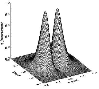
Figure 10: Instantaneous beam of $\perp$-mode curvature radiation (power per unit frequency per unit solid angle) as a function of the angle $\psi$, measured from the plane of a $B$-field line, and the angle $\mu$ measured in the orthogonal way. The vector of electron velocity (not shown) is anchored at the origin of the reference frame and points vertically upward, along the local magnetic field. There is no radiation in the plane of the electron trajectory, which is the plane of $\psi=0$.

As shown in DRR the PAC maser is unable to naturally produce double notches with the observed depth of $\ga 20\%$ (Perry & Lyne 1985). This is because the PAC beam has the hollow cone shape, and is axially symmetric around the local electron velocity (around the local $\vec{B}$). Therefore, a ring-shaped part of the emitter contributes to the flux that is observed at the minima of notches and makes them very shallow. For a two-dimensional emitter that extends laterally at a fixed altitude, this ‘light-polluting’ ring has the crossection which is marked with letters ‘b’ in fig. 3 of DRR.

In the case of the $\perp$-mode curvature radiation, the beam has the mirror symmetry with respect to the plane of the local $B$-field line, and there is no (or little) emission within the entire plane (see Figs. 10 and 11). Each point of emission region is therefore mostly emitting in only two directions, which make small angles $\psi_{\rm max}$ with respect to the plane of the $B$-field line (note that in the case of the low-frequency curvature radiation $\psi_{\rm max}\gg 1/\gamma$). Therefore, instead of the ‘polluting ring’, there are only two spots in the emission region (on both sides of the absorber) that contribute to the flux observed at the minima of double notches. The minima are therefore much less contaminated by the nearby parts of the emitter than in the PAC case. Moreover, the eclipsing object does not longer need to be compact. Overlying opaque streams (Fig. 12), or elongated disruptions in the emitter, can produce deep notches without affecting the flux at the center of the notches. In the curvature scenario deep double notches are therefore produced easily and naturally.

Fig. 11 schematically shows how the split-fan beam due to a thin stream is created: when electrons move along the curved magnetic field lines they carry-along the two-directional pattern of Fig. 10. The resulting beam has therefore completely different structure (split fan) than the parallel-acceleration beam (hollow cone). It is precisely this topological property that really makes the crucial difference, and allows us to recognize which mechanism is the correct one.

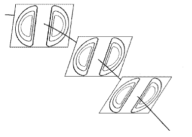
Figure 11: The beam of the previous figure is carried by the electron along a magnetic field line, which produces the two-planar, split-fan beam. The fixed-intensity contours of the instantaneous beam are shown at three locations on a magnetic field line.

The ease with which the $\perp$-mode curvature beam produces deep double notches, was verified with a 3D numerical simulation. The code assumes that the emitter has the shape of a surface formed by magnetic field lines with fixed footprint parameter $s$. The footprint parameter is arbitrarily fixed at $s=1$ (last open field lines). To produce the omnipresent ‘pedestal’ emission, the curvature radiation continues up to a quite high altitude of $(2/3)R_{\rm lc}$.

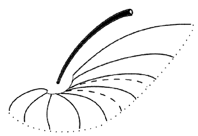
Figure 12: Natural geometry that produces deep double notches. An opaque stream (black arc) is located above a two-dimensional emission region. The solid lines present magnetic field lines. Two dashed lines trace the eclipsed parts of the emitter.

The most natural way to generate the notches is shown in Fig. 12 and involves a thin opaque stream of plasma above our emission region. We call it most natural because we know that such streams exist and produce the BFC. Note that because the notches are observed in averaged profiles, the obscuring stream has to be fairly permanent to be present in the same pulses as the emission which is absorbed. However, to simplify the calculations we preferred to model an elongated fissure in the emitter, instead of the obscuring stream. Thus, we assumed that a narrow part of the emitter (a wedge with a fixed angular width of $\Delta\phi_{m}=4.1^{\circ}$ in the magnetic azimuth) is not emitting. This is a safe assumption, since the ability to produce deep notches does not depend on whether they are produced by an absorber above, or the hole within the emission region (DRR).

The simulations have confirmed that deep double notches appear naturally for the $\perp$-mode curvature beam. A sample result for three different viewing angles is shown in Fig. 13. It also becomes clear now why the notches can only be observed in very highly polarised pedestal emission: when the $\parallel$-mode is present, it fills-in the central minimum of the double $\perp$-mode beam and the notches cannot appear.

Based on Sections 3 and 4 we learn that in the case of curvature radiation, both the double absorption features (double notches) of several pulsars as well as the bifurcated emission components of J1012$+$5307 and J0437$-$4715 can be understood in terms of natural geometry that involves the absorption/emission by plasma streams in pulsar magnetic field. We conclude that it is the curvature radiation, not the radiation due to the parallel-acceleration, that is observed as the coherent radio emission from pulsars.

Figure 13: Deep double notches simulated with a 3D numerical code. The background (pedestal) emission was created by the surface of last open field lines. A wedge-shaped part of the surface was not emitting to produce the notches. The wedge was centered at the magnetic meridian $\phi_{m}=-20^{\circ}$, and had the azimuthal width of $\Delta\phi_{m}=4.11^{\circ}$. The curves correspond to $\zeta=64.3^{\circ}$, $51.5^{\circ}$, and $38.6^{\circ}$ (top to bottom). The magnetic dipolar field was tilted at the angle $\alpha=90^{\circ}$.

5 Polarisation structure of the curvature beam

To consider some implications of our findings, we first discuss the polarisation structure of the two-modal curvature beam.

It is convenient to imagine the ‘elementary’ beam as the fan beam due to the passage of an electron along a magnetic field line (or due to a thin stream flowing along a narrow bunch of $B$-field lines). Based on the fits of Section 3 it is reasonable to assume that the $\perp$-mode beam is amplified isotropically and preserves the original (non-coherent shape). The $\parallel$-mode beam is likely to be attenuated in the central parts (near $\psi\sim 0$), where the radiation propagates through the largest plasma density. The outer parts of the $\parallel$-beam are emitted from the outer boundary of the stream into the low-density region surrounding the stream. Guided by the observed edge depolarisation of profiles (see Section 6.2) we assume that in the outer wings of the beam, the $\parallel$-mode radiation is amplified with the same efficiency as the $\perp$-mode and is not attenuated.

The polarisation-structure of such a toy beam is shown in Fig. 7a with thick lines (solid for $\perp$-mode, dot-dashed for $\parallel$-mode). Three cases of $\parallel$-mode attenuation are shown, marked with $\parallel$A, $\parallel$B, and $\parallel$C. Since the $\perp$-mode has zero emissivity in the ET plane, even a small contribution of $\parallel$-mode (shown as the case $\parallel$B) can dominate the central parts of the total beam. It is also possible to have the $\parallel$-mode fully absorbed in the beam center (case $\parallel$C). Such half-phenomenological curvature-radiation beam has several intrinsic properties that make it notably successful in interpreting enigmatic pulsar phenomena.

6 Application to selected pulsar problems

6.1 Polarised multiple imaging

The inferred polar carousel of many pulsars exhibits interesting structure in magnetic azimuth $\phi_{m}$: subbeams of opposite orthogonal polarisation are distributed alternatingly along the polar ring of emission. This pattern produces several enigmatic phenomena, such as 1) the “modal parity at the outside edges of polar beam” (Rankin & Ramachandran 2003), 2) two orthogonally-polarised, out-of-phase drift patterns, 3) jumps in drift phase (Edwards 2004). The latter two effects were described by Edwards, Stappers & van Leeuwen (2003) as ‘multiple imaging’ possibly caused by refraction, birefringence or aberration/retardation effects.

Without intending to model the phenomena in detail, we want to show that the low-frequency curvature radiation beam has several intrinsic properties that are consistent with the observations. First, the multiple imaging is automatically implied by the non-zero angular width of the low-frequency beam of curvature radiation:

$$\psi_{\rm max}\simeq 0.62\left(\frac{3c}{2\pi\rho\nu_{\rm obs}}\right)^{1/3}=0.40^{\circ}(\rho_{7}\nu_{9})^{-1/3},$$ (14)

where $\rho_{7}=\rho/(10^{7}$ cm), and $\nu_{9}=\nu_{\rm obs}/(1\ {\rm GHz})$. One can see that for the typical radius of curvature of $10^{7}$ cm, the intrinsic width effects become important/noticeable right in the lower part of the standard frequency band of radio astronomy ($\nu_{\rm obs}<1$ GHz). Any intrinsic broadening of components that is smaller than $\sim$$1^{\circ}$ would be hard to notice in pulse profiles. Thus, by transiting from sub-GHz to super-GHz radio band one goes from profiles dominated by intrinsic shape of the curvature-radiation beam (with the radiation emitted at noticeable angles with respect to $\vec{B}$) to profiles dominated by the spatial distribution of emission region (with the emission tightly bound to the direction of $\vec{B}$). At fixed $\nu_{\rm obs}$ the intrinsic broadening depends only on the curvature radius $\rho$ and the dependence is rather weak ($\propto\rho^{1/3}$). This explains why the scale of double features is so similar in so different objects like the millisecond pulsars (MSPs) and normal pulsars. On the other hand, $\rho$ is a bit smaller in MSPs and the strongly flaring $B$-field lines make it possible to observe the double emission components well-isolated from the main pulse. Therefore, the double emission features are most easily noticed in MSPs. The scale of double absorption features (notches) additionally depends on the eclipsing geometry and will be analysed elsewhere. We conclude that the multiple imaging effect is naturally guaranteed by the non-zero width of the curvature beam at low $\nu_{\rm obs}$. No refraction, birefringence etc. is needed in the zeroth-order approach to understand the multiple imaging.

6.1.1 A method to determine the curvature of electron trajectory in the emission region

At a fixed and low observation frequency ($\nu_{\rm obs}\leq\nu_{\rm crv}$), the opening angle $\psi_{\rm max}$ of curvature emission depends only on the curvature radius of electron trajectory in our (observer’s) reference frame. This opens a way to calculate the curvature radius $\rho$ in the emission region from eq. (14). However, this can only be achieved when full information on the global geometry of the system is available. Since the viewing angle $\zeta$ can be different than $90^{\circ}$, the observed separation of maxima in the BFC can be rescaled (increased) by the factor $1/\sin\zeta$ due to the well-known ‘not-a-great-circle’ effect. Moreover, if the plane of the electron trajectory is inclined at an angle $\delta_{\rm mdn}$ with respect to the local meridional plane the value of $\Delta_{\rm bfc}$ is increased by additional factor $1/\cos\delta_{\rm mdn}$. One can also use the factor $1/\sin\delta_{\rm cut}$, where $\delta_{\rm cut}=90^{\circ}-\delta_{\rm mdn}$ is the angle at which we cut the ET plane. The observed $\Delta_{\rm bfc}$ is therefore related to $\psi_{\rm max}$ through the global geometry parameters:

$$\Delta_{\rm bfc}\simeq\frac{2\psi_{\rm max}}{\sin\zeta\cos\delta_{\rm mdn}}=\frac{0.8^{\circ}}{\sin\zeta\sin\delta_{\rm cut}(\rho_{7}\nu_{9})^{1/3}}.$$ (15)

Therefore:

$$\rho_{6}=\left(\frac{1.72^{\circ}}{\Delta_{\rm bfc}}\frac{1}{\sin\zeta\sin\delta_{\rm cut}}\right)^{3}\nu_{9}^{-1},$$ (16)

where $\rho_{6}=\rho/(10^{6}\ {\rm cm})$. For J1012$+$5307 we have $\Delta_{\rm bfc}=8.61^{\circ}$ and $7.1^{\circ}$ at $0.82$ and $1.4$ GHz respectively, which implies $\rho\sin^{3}\zeta\sin^{3}\delta_{\rm cut}\simeq 0.011\cdot 10^{6}$ cm at both frequencies. To make $\rho$ equal to $10^{6}$ cm, either $\zeta$ or $\delta_{\rm cut}$ of $\sim$$13^{\circ}$ is required. For moderate values of $\zeta=\delta_{\rm cut}\simeq 45^{\circ}$, the value of $\rho$ is increased by a factor of $8$ up to $\sim$$0.1\cdot 10^{6}$ cm.

Note that the small value of $\rho\sin^{3}\zeta\sin^{3}\delta_{\rm cut}$ does not have to necessarily imply sub-stellar curvature radius. The main pulse of J1012$+$5307 has the width that corresponds exactly to the opening angle of low-altitude polar tube, and the interpulse is present. This suggests orthogonal viewing geometry ($\zeta\sim\alpha\sim 90^{\circ}$). However, this kind of geometry simultaneously necessitates small cut angles ($\delta_{\rm cut}\sim 0^{\circ}$) for components observed well ahead of main profile features (main pulse and interpulse).

In the case of J0437$-$4715, we have $\Delta_{\rm bfc}=3.76^{\circ}$, $2.89^{\circ}$, and $1.7^{\circ}$ at $0.438$, $0.66$ and $1.512$ GHz, respectively. This gives $\rho\sin^{3}\zeta\sin^{3}\delta_{\rm cut}=0.22$, $0.3$, and $0.7\cdot 10^{6}$ cm, respectively. The results for J0437$-$4715 are closer to what we expect for dipolar magnetic field lines. The actual $\rho$ is probably larger, because $\zeta\la 45^{\circ}$ is likely. On the other hand, the BFC of J0437$-$4715 has a very shallow central minimum due to some convolution effects (eg. due to the $\vec{E}\times\vec{B}$ drift of the stream). This can make $\Delta_{\rm bfc}$ appear slightly smaller.

It is worth to digress here into the phase location of BFCs in pulse profiles. The precursor location of both BFCs observed in J1012$+$5307 (at $\phi\simeq 71^{\circ}$ and $245^{\circ}$ in Fig. 2) is reasonable, because for fast-rotating pulsars with large dipole inclination, radiation emitted from any altitude cannot be detected far on the trailing side of the main pulse. Because of the effects of aberration and retardation, the latest-possible phase of detection is equal to the caustic phase of $16^{\circ}s^{2}/\sin^{2}\alpha+\phi_{f}$, where $s$ is the footprint parameter of $B$-field lines and $\phi_{f}$ is the absolute fiducial phase (Dyks, Wright & Demorest 2009, in preparation). J0437$-$4715 does not obey this ‘precursor rule’, probably because of much smaller dipole inclination ($\alpha\ll 90^{\circ}$, $\zeta\ll 90^{\circ}$).

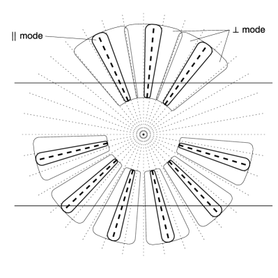
Figure 14: In the case of the curvature radiation with partially-absorbed $\parallel$-mode, the carousel of electron streams (thick dashed) naturally produces polarisation pattern in which the two orthogonal modes dominate alternatingly in magnetic azimuth. The thick contours present the $\parallel$-mode, the thin contours are for the $\perp$-mode, and the $B$-field lines are dotted. The two horizontal lines mark two different ways in which our line of sight can leave the beam: in the case shown at the top the sightline cuts through the fixed-azimuth outer boundary of an azimuthally-limited emitter.

6.1.2 Azimuthal separation of orthogonal modes

The plane of $\psi=0$, (orthogonal to the page in Fig. 7a), is the plane of symmetry of the curvature beam. Such fan beam has therefore intrinsic mirror symmetry with respect to the plane of $B$-field lines. In the case of the partial contribution of the $\parallel$-mode (case $\parallel$B in Fig. 7), the two orthogonal polarisation modes are naturally separated in magnetic azimuth: the $\parallel$-mode dominates in the plane of the $B$-field lines, whereas the $\perp$-mode dominates on both sides of the parallel mode. This provides a very natural way to obtain the azimuthally-structured polarised carousels observed by Rankin et al. (2006) and Edwards et al. (2003).

Let us assume the usual picture in which the polar region is populated with thin plasma streams that are separated in magnetic azimuth and are anchored to the sparking spots (the carousel of Ruderman & Sutherland 1975). In such a case, the geometry of the curvature beam contaminated by the $\parallel$-mode assumes the shape shown in Fig. 14. The thin plasma streams (actually only their fragments that emit detectable radio waves) are marked with thick dashed lines. The $\parallel$-mode emission (dominating within, but not constrained to, the planes of the streams) is delineated with thick solid contours. The $\perp$-mode emission flanks the sides of the $\parallel$-mode beam (thin contours). The pattern naturally results from the intrinsic properties of the curvature beam with not-fully-absorbed $\parallel$-mode. Thus, the azimuthal separation of modes can appear even with no refraction nor birefringence involved.

Note that Fig. 14 presents the instantaneous geometry of emitting streams, and refers to single pulse data after they have been deconvolved into the image of polar carousel. In the averaged pulse profile, the structure of Fig. 14 is likely to become smeared out by plasma drift effects. The exact outcome of such averaging depends on the relative speed of drift motion and pulsar rotation.

6.2 Edge depolarisation of profiles

Rankin & Ramachandran (2003) emphasized the significant observation that the outer edges of pulsar profiles are almost totally depolarised. Thus, some high-level conspiracy between the modes seems to be required. The curvature radiation is an extremely likely cause of this conspiracy, because it intrinsically emits equal amounts of the orthogonal polarisation states in the outer edges of the curvature beam. For $\psi\gg\psi_{\rm max}$, we have $\xi=1/\gamma^{2}+\psi^{2}\simeq\psi^{2}$, and $K_{\frac{2}{3}}(y)\simeq K_{\frac{1}{3}}(y)$, so the eq. (4) implies:

$$\eta_{\perp}/\eta_{\parallel}=1.$$ (17)

This ratio, as well as the polarisation degree $L/I$, are shown as a function of $\psi$ in Fig. 7b. The decrease of $L/I$ with the angular distance from the symmetry plane (increasing $|\psi|$) is readily apparent.

The well-known problem is that the emitted curvature radiation is polarised elliptically. It is not only limited to the two orthogonal modes. So some mechanism is needed to filter out the purely-orthogonal modes. Whatever mechanism actually does it, a seemingly natural way to have equal amounts of two strictly-orthogonal modes, is to filter them proportionally out of a beam that already (intrinsically) includes equal amounts of radiation in the two orthogonal polarisation states. The curvature emission is then an ideal candidate, because in the outer wings of the elementary beam, it intrinsically produces equal amounts of radiation in the appropriate polarisation states. We therefore claim that the observed edge depolarisation has its origin in the intrinsically equal emissivity in both polarisation states. Our line of sight can pass through the pulsar beam shown in Fig. 14 in two ways, marked with the horizontal lines. In the bottom case (grazing the edge of the carousel) it is probably a bit difficult to guess the averaged polarisation degree without numerical simulation. In the top case, however, the polarisation degree at the edge of the profile will decrease, because our line of sight moves away from the fixed-azimuth plane of the last-seen emitter ($|\psi|$ in Fig. 7b increases).

6.3 The origin of double conal profiles

An interesting question is what happens when the stream has noticeable azimuthal width, that is comparable to (or larger than) the opening angle $\psi_{\rm max}$. We argue that a cut through such stream produces the double conal profiles (type D in the classification scheme of Rankin 1983). A geometry of such a cut is presented in the bottom right corner of Fig. 18. The brightening of the edges of the profile is caused by the increased contribution of $\parallel$-mode. The near-absence of the $\parallel$-mode in the inner parts of the profile leads to the smaller flux and large polarisation degree. The presence of the $\parallel$-mode at the flanks of the profile also produces the depolarisation. In some cases, when sufficiently large amount of the $\parallel$-mode gets through, orthogonal jumps of averaged polarisation degree are observed in the outer wings of a pulse (eg. B1133$+$16, B2020$+$28, B2053$+$21, Hankins & Rankin 2008, hereafter HR08).

The nearly-complete depolarisation of profile’s edges is ensured by the fact that our line of sight passes through a region with limited magnetic azimuth (as can be seen in Fig. 18 the sightline enters/exits the fixed-azimuth sides of the elongated wedge). It is not passing through a conal ring centered at the dipole axis. The brightest parts of the emission region (and the peaks of a profile) correspond to the fixed value of $\phi_{m}=\phi_{m}^{\rm le}$ on the leading edge and to $\phi_{m}=\phi_{m}^{\rm te}$ on the trailing edge of the wedge-shaped stream. When our line of sight departures from the fixed-$\phi_{m}$ edge, it moves away from the center of the curvature beam shown in Fig. 7a. The polarisation degree is therefore decreasing as shown in Fig. 7b.

6.3.1 The origin of the radius-to-frequency mapping

The interpretation here implies that the observed pulse width $W$, as measured between the profile peaks is fixed by the extent of the emitter/stream in the magnetic azimuth: $\Delta\phi_{m}=\phi_{m}^{\rm te}-\phi_{m}^{\rm le}$. In the zeroth-order consideration this implies the lack of pulse broadening at low frequencies. Some of the D-type pulsars indeed exhibit no widening within a huge frequency range (eg. B0834$+$06 between $\sim 25$ and $2370$ MHz, see Fig. 4 in HR08), but some definitely do (eg. B0301$+$19).

However, on a closer inspection the widening (mis-interpreted as RFM) can appear at low frequencies, since the plasma density in the stream falls off with the transverse distance from the stream center/axis. So we assume that the basic principle of the broadening is the same as usual: low-$\nu_{\rm obs}$ radiation emerges from regions with lower density. However, the lower density regions in our scenario are simply the more extreme outskirts of the stream, ie. the lower-density region located further away from the stream axis. Thus, we replace the ‘radius-to-frequency’ mapping with the ‘stream-diameter-to-frequency’ mapping. This interpretation implies that all radio frequencies come from the same (or similar) range of altitudes.

6.3.2 The origin of the S-swing of polarisation angle

Figure 15: a) Decomposition of a D-class profile into elementary beams emitted from different locations in the plasma stream. The $\perp$-mode-dominated beam (thick line) is emitted from the center, and the $\parallel$-mode-contaminated, asymmetric beams from the outside edges (thin lines). In the phase-interval C the variations of polarisation angle are determined by the intrinsic properties of the elementary beam (see text for more details). b) Plasma density distribution sampled by our line of sight. The short bars mark the emission points for the curves in panel a.

The small width $\Delta\phi_{m}$ of the emitter in the magnetic azimuth implies that the projected direction of magnetic field does not change much within the pulse window. Thus, our scenario implies almost no change of polarisation angle (PA) due to the effect predicted by the rotating-vector-model (RVM) of Radhakrishnan & Cooke (1969). The PA curve is predicted to stay flat only if it is dominated by the RVM effect, ie. if the observed PA is determined by the projection of $\vec{B}$ on the sky. If the PA is governed by non-RVM factors, then behaviour that is in general different from the RVM curve is expected.

The non-RVM behaviour is indeed observed in several pulsars with double peaks. For example, this is the case for B0834$+$26, B1919$+$21 (HR08), as well as for the geodetically-precessing pulsar B1913$+$16 (see fig. 7 in Weisberg & Taylor 2002). However, the non-RVM origin seems to be plain inconsistent with the paramount examples of the RVM exhibited by two well-known representatives of the D-class: B0301$+$19 and B0525$+$21. They are widely believed to present textbook cases of the RVM-generated PA curve.

We claim that here again we become victims of maliciously deceiving degeneration of Nature. The RVM model is really what the name says: a curve determined by the sky-projection of a vector that rotates under our line of sight. The projection of the circumpolar $B$-field lines is just one example of such a vector. The other examples, not even slightly less natural than the projected $\vec{B}$, are the vectors of electric field in the radiation pattern surrounding the instantaneous velocity of a relativistic particle. We argue that the famous S-swing of PA in the B0525$+$21 (and other D pulsars) is mostly caused by intrinsic effects. It is due to the cut of our sightline through the elementary (microscopic) $\perp$-mode curvature beam.

A rather complicated code would be needed to prove it numerically. Instead of that, we choose to delinate the mechanism qualitatively. In Fig. 15a the observed pulse profile of a D-class pulsar is decomposed into the elementary beams, emitted from three locations in the stream. The thick curve presents the bifurcated $\perp$-mode-dominated beam emitted from the center of the stream. The thin lines on the left- and right-hand side present the beams emitted from the outside left and right edge of the beam, respectively. The edge beams have their outside parts brightened by the presence of the $\parallel$-mode. Within the phase interval marked with the letter ‘A’, the polarisation properties are determined by relative proportions of the two modes. If the segregation of the modes is not efficient in 100%, a substantial elliptical polarisation appears there (as is often observed). In the phase interval ‘B’ the flux observed at each phase always corresponds to the maximum of different elementary beams, emitted at different locations in the stream. The changes of PA within the interval ‘B’ are therefore dominated by the changes of the $\vec{B}$ field direction. Thus, it is in the phase interval B, where the emission from different elementary beams is averaged out and can reveal the underlying geometry of magnetic field. In this interval the observed average PA curve can follow the RVM model. This can only happen if the width of the phase interval B is noticeably large (the width is determined by the relative width of the stream and the opening angle $\psi_{\rm max}$ of the $\perp$-mode beam). The corresponding parts of the PA curve of B0525$+$21 are indeed very flat (and highly polarised because of the domination of the $\perp$-mode).

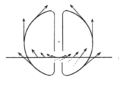
Figure 16: The origin of the PA swing in D-type radio pulsars. A head-on view of the $\perp$-mode curvature beam with the orientation of polarisation vectors marked at selected places. The passage of observer’s line of sight (horizontal line) leads to identical PA swing as in the case of the RVM model.

In the phase interval ‘C’ the situation changes completely: for $\phi<0$ the flux at each phase is now dominated by radiation from a single elementary beam. Our line of sight does not sample different beams emitted from different locations in the stream. The sightline moves through the inner parts of the elementary beam, and the changes of PA are determined by the changes of polarisation direction intrinsic to the $\perp$-mode beam (note that in this phase interval the received radiation is associated with a fixed direction of $\vec{B}$). For $\phi>0$ (still in the C interval), the line of sight again samples a single elementary beam. Therefore, in the innermost parts of the double conal profiles, the PA is determined by the intrinsic polarisation properties of the $\perp$-mode curvature beam. As shown in Fig. 16, the orientation of the polarisation vectors (vectors of the electric field $\vec{E}_{w}$ of the emitted wave) in the instantaneous $\perp$-mode-beam ensures the same variations of the PA as the projected magnetic field in the RVM model. This interpretation is based on the intrinsic properties of the emitted radiation and assumes that they are not affected by any adiabatic walking below the polarisation-limiting radius (eg. Cheng & Ruderman 1979; Melrose 1979; Lyubarsky 2002).

We thereby disclose a perverse situation, in which the central parts of the observed PA curve, that resemble the RVM shape so closely, have the origin that has nothing to do with the RVM idea. On the contrary, the outer flat parts of the observed PA curve (interval B) are more likely to reflect the underlying orientation of $\vec{B}$ and to comply with the RVM origin. Had this been the case, the difference of PA measured in the outer wings of the profile $\Delta(\rm PA)$ would provide information about the azimuthal width of the stream: $\Delta\phi_{m}\sim\Delta(\rm PA)$ (provided the PA observed in the A and B region is not biased/dominated by intrinsic effects).

The same conclusion can be reached in a different way, by considering the case of an infinitely-thin stream, and noting that the observed PA curve should change continously for small increase of the stream width. Specifically, for a stream of electrons flowing only along a single $B$-field line, the observed PA curve definitely has to be determined fully by the intrinsic swing shown in Fig. 16. This is because the spatial extent of the emitter is a delta function and there is no variation of the underlying direction of $\vec{B}$. A small increase of the diameter of the stream must, by continuity, produce only small changes of the initial PA curve. The increasing spread of $\vec{B}$ within the stream of increasing thickness will therefore produce only a gradual change in the observed PA curve. We therefore conclude that in general the observed PA curves of pulsars are a convolution of intrinsic PA and $B$-field projection.

Since the opening angle of the $\perp$-modecurvature beam decreases with increasing frequency, the PA curve is expected to depend on $\nu_{\rm obs}$, which is indeed the case for B0525$+$21 (and other objects). Because the $\perp$-mode-radiation has a minimum in the profile center (Fig. 15), any remnants of the $\parallel$-mode emission can produce a minimum of polarisation degree there. Even such detail is also observed in B0525$+$21 (eg. fig. 1 in HR08). In a more general case (than the primitive picture of Fig. 15), a large variety of PA curves is expected, depending on the 3D distribution of plasma density in the stream, on the geometry of passage of our sightline through the beam, on the ratio of both orthogonal modes, and on the size of the elementary curvature beam. For realistic density distribution the phase intervals B and C can overlap in phase, in which case the PA recorded at a given phase can be partly determined by the intrinsic PA and partly by the projection of $\vec{B}$. The subject deserves numerical study.

Interesting examples of intrinsic variations of PA curve have also been observed under core components, where the polarisation has been found to depend on the subpulse brightness (B1237$+$25, Srostlik & Rankin 2005; B0329$+$54, Mitra, Rankin & Gupta 2007). The core emission has been found to be polarised orthogonally with respect to the outer components (Srostlik & Rankin 2005) which suggests $\parallel$-mode origin of the core (Gil & Snakowski 1990).

We conclude that the observed PA curve (at least for D-type pulsars) is strongly influenced by the intrinsic polarisation properties of the $\perp$-mode-beam. Even in the most RVM-like looking fragments it does not have the RVM orgin. Though this interpretation invalidates the determination of the general geometric parameters ($\alpha$, $\zeta$) from the PA curves, it opens a way to interpret their ubiquitous distortions from the RVM-shape.

6.3.3 Profile width and the geodetic precession

Precessing pulsars give us the unique opportunity to view their emission beams in two dimensions. Especially precious are the pulsars in relativistic binary systems, such as J0737$-$3039A/B, B1913$+$16, J1141$-$6545, B1534$+$12, or J1906$+$0746. They should exhibit the geodetic precession, the rate of which is well determined by the general relativity. For the traditional, axially-symmetric pulsar beams, such precession should generally produce clear changes of profile width. Several detailed studies of the phenomenon (Kramer 1998; Clifton & Weisberg 2008; Lorimer et al. 2006; Burgay et al. 2005) have reported that the profiles refuse to change at the expected rate. This suspicious observation can be explained in several ways, eg. by near-alignment of the spin axis and orbital angular momentum, or by the accidental approximate co-planarity of the rotation axis, orbital momentum, and line of sight (see Clifton & Weisberg 2008). However, none of the explanations seems natural or likely, especially in view of the increasing ubiquity of the problem.

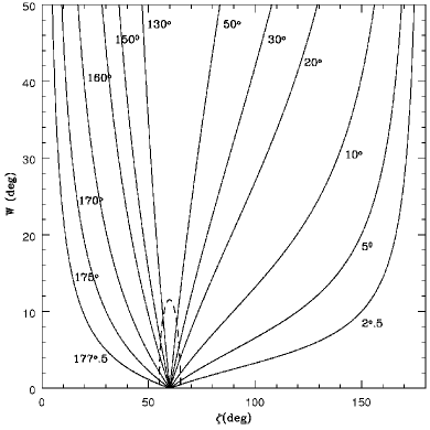
Figure 17: Variations of pulse width $W$ as a function of the viewing angle $\zeta$ in the stream model (solid lines; numbers give the value of $\phi_{m}=\Delta\phi_{m}/2$). The outermost two curves present the thinnest streams of width $\Delta\phi_{m}=5^{\circ}$ and $10^{\circ}$ in the magnetic azimuth. The streams are centered at the main meridian and $\alpha=60^{\circ}$. Dashed line presents the standard case of a conal beam with the opening angle $2\theta_{m}=10^{\circ}$.

We argue that the real reason for the profile stability is the completely different topology of pulsar beams: our sightline is cutting through the split/structured fan beams generated by elongated plasma streams, not through the narrow cones. The pulse profile of B1913$+$16 indeed has the D-class shape and exhibits strongly distorted (non-RVM) PA curve (fig. 7 in Weisberg & Taylor 2002). However, our fan-beam interpretation is likely to hold not only for the D-class profiles. The pulsar J1906$+$0746 (Lorimer et al. 2006) belongs to a single-component class (S type), and exhibits interesting profile evolution: despite its interpulse clearly appearing within a few-years-long observation time, the width of the main pulse does not vary considerably. A cut through fan-beams explains such behaviour naturally.

In the traditional conal model the observed pulse width $W=2\phi$ is modelled by assuming the fixed opening angle $\theta_{m}$ of the conal beam in the equation:

$$\cos\phi=\frac{\cos\theta_{m}-\cos\alpha\cos\zeta}{\sin\alpha\sin\zeta}.$$ (18)

In the fan beam scenario it is the azimuth $\phi_{m}$ of a wedge-shaped stream that needs to be fixed, whereas $\theta_{m}$ in the above formula changes with time, complying with the equation:

$$\cos\zeta=\cos(\pi-\phi_{m})\sin\alpha\sin\theta_{m}+\cos\alpha\cos\theta_{m}.$$ (19)

The assumption of $W=2\phi$ is only correct for a stream that is symmetric with respect to the main meridian (containing the rotation and magnetic axes). In general, $\phi_{m}^{\rm le}\neq\phi_{m}^{\rm te}$ and the width is equal to $W=\phi(\phi_{m}^{\rm te})-\phi(\phi_{m}^{\rm le})$, with $\phi$ given by eq. (18). The instantaneous value of $\cos\theta_{m}$ needs to be calculated from the quadratic equation (19) and used in (18). This leads to the much slower variations of $W$ with $\zeta$, as can be seen in Fig. 17 in which the solid lines show $W$ for streams of various azimuthal width $\delta\phi_{m}=2\phi_{m}$ and $\alpha=60^{\circ}$. The quasi-linear changes of $W$, characteristic for the observations of geodetically-precessing pulsars, are readily apparent for narrow streams (outermost lines; see the values of $\phi_{m}$ marked at each line). The changes of $W$ for a conal beam with $\theta_{m}=10^{\circ}$ are shown for comparison with the dashed line.

Therefore, because of the geodetic precession we have already traversed a long way through the beam of B1913$+$16. The profile has not evolved much because we cut through a fan-shaped beam. We argue that the stability of profile in both components of the double pulsar J0737$-$3039A/B has the same origin, despite the profile classification for the A star is far from clear.

6.4 Sketch of a new classification scheme

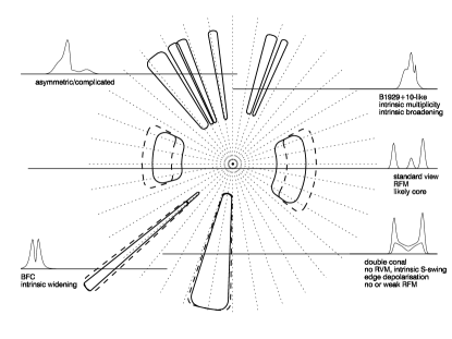
Figure 18: A head-on view down the magnetic pole, presenting the geometry of possible emission regions. Some of them are plotted at two frequencies: a lower one (dashed contours) and a higher one (solid contours). The standard conal view of profile generation (middle sightline) is contrasted with the stream origin that we advance in this paper (bottom sightlines). The stream-cut origin is likely not restricted to the D-class pulsars, as suggested in the upper part of the figure.

6.4.1 Neither conal nor patchy: spoke-like, wedge-like, and stream-like

We have come to the conclusion that bifurcated components in radio-pulsar profiles are produced by sightline cuts through fan-beams of radiation from elongated streams. There need to be stream-like emitters in the pulsar magnetosphere, as shown in the bottom-left corner of Fig. 18. An important question is what is the length of the streams and what is the range of magnetic colatitudes that the fan beams subtend. At least in some cases the fan-beams must extend quite far from the dipole axis, to explain the large separation of bifurcated components from the main parts of the profile (main pulse, interpulse). The large extent could also explain the abundance of pulsars with interpulses (eg. Weltevrede & Johnston 2008b). If the streams are not exactly centered at the main meridian, the main-pulse-interpulse separation can differ from $180^{\circ}$ as it sometimes happens to be observed (eg. in B1055$-$52, Weltevrede & Wright 2009).

The components of the BFC class are observed at frequency-independent location in pulse profiles and widen with increasing $\nu_{\rm obs}$ roughly according to $\Delta_{\rm bfc}\propto\nu_{\rm obs}^{-1/3}$.

For the price of rejecting the RVM wisdom, we have also come to the conclusion, that the double conal profiles (class D) are also created by a cut through azimuthally-limited emitter, that is a bit broader than in the BFC case (right bottom corner of Fig. 18). The width of such profiles is mostly determined by the fixed width of the stream. Any low-frequency widening (of non-RFM nature) can result from density gradient in the outskirts of the stream. The intrinsic $\nu_{\rm obs}^{-1/3}$ widening can also contribute to the apparent effect.

The fan-beam origin of pulse profiles is probably not limited to the D class. The profile of B1929$+$10 is likely created by a cut through a structured stream, or through a few nearby streams. At 430 MHz, its profile has a pronounced emission component on the trailing side of the maximum, which separates from the maximum at a rate roughly consistent with $\nu_{\rm obs}^{-1/3}$. Moreover, in the minimum between the component and the central maximum, noticeable amount of orthogonal polarisation mode appears (Rankin & Rathnasree 1997). This kind of corellation (appearance of another polarisation mode at a minimum in total flux) could in principle be produced by any process that removes the dominating mode. However, here we find again that the $\perp$-mode-dominated curvature beam (case $\parallel$B in Fig. 7a) has the appropriate intrinsic property to produce the phenomenon (domination of the $\parallel$-mode at the minimum of the $\perp$-mode). We therefore suggest that the ‘multiple’ appearance of the profile of B1929$+$10 is partially caused by the intrinsic doubleness of the curvature beam, and the real number of underlying streams is smaller than the number of observed components. If the radiation in the pedestal emission is averaged out to reveal the RVM polarisation angle, then this pedestal PA curve should be discordant with the PA curve observed under the main pulse (because the latter is dominated by intrinsic effects). This likely explains the difficulty in fitting the full-period interval with a single PA curve (Rankin & Rathnasree 1997; Everett & Weisberg 2001). B0950$+$08 may belong to the same, B1929$+$10-like class: its profile tends to bifurcate at low $\nu_{\rm obs}$. The extended leading-bridge of this profile is likely caused by a stream that extends roughly tangentially to the trajectory made by our line of sight. The bridge culminates in an interpulse which again reveals doubleness (McLaughlin & Rankin 2004).

A paramount example of stream-cut-generated profile is provided by J0437$-$4715 in which the tendency to ‘look double’ is revealed both in the complicated central parts and in the conal components. Whereas the core can be produced in the usual way (a cut through the dipole-axis-centered rings) it may also be created by streams flowing near the main meridian. The outer “conal” components are definitely produced by streams with large $\phi_{m}$. Deconvolution of this (and other) profiles into the underlying emitting structures (streams) can only be done if the bifurcated nature of the elementary curvature beam is taken into account.

7 Summary

The bifurcated component of J1012$+$5307 can be comparably-well fitted with both the parallel-acceleration emission and the curvature radiation. However, only the curvature radiation can match the data simultaneously at two frequencies. The two-planar topology of the $\perp$-mode-dominated curvature beam makes it very easy to reproduce the observed large depth of double notches. It also explains the origin of bifurcated components in terms of very natural geometry (sightline cuts through plasma streams). This leads us to the firm conclusion that the observed coherent radio emission from pulsars is the curvature radiation.

Components in radio pulsar profiles become wider, and finally bifurcate at low-frequencies because of the intrinsic behaviour of the curvature beam. The scale of the bifurcation makes it possible to determine the radius of curvature of electron trajectory in the emission region, provided global geometry parameters are known.

Double “conal” profiles (D class) are not conal in the usual sense. They are produced by the sightline cut through slightly broader streams.

The PA curves of such profiles are not determined by the projection of the $\vec{B}$-field on the sky plane. Even when they resemble the RVM shape (which they do rarely), the PA curves are mostly determined by the microphysical polarisation structure of the $\perp$-mode curvature pattern. The S-swing created by a cut through such single pattern is exactly the same as in the RVM case. Angular/spatial convolution of more patterns leads to a variety of observed PA curves.

The low-frequency broadening of D-type profiles results from plasma density gradient at the outer surface of the stream, and from the intrinsic broadening of the curvature beam. It does not reflect the emission radius (it does not have the RFM origin).

The narrow-stream geometry of the emitter implies fan-like shapes of pulsar emission beams. This naturally explains the extremely slow changes of pulse width due to the geodetic precession.

The existence of fan-shaped beams increases the likelihood of observing an interpulse. It also implies that the number of pulsars in the Galaxy may be smaller than estimated with the conal beams.

The results of this paper invalidate the traditional methods of determination of the radio emission altitude at least for D-class pulsars. This refers both to the geometrical method, and the one based on the relativistic-shift of PA curve.

The curvature-radiation beam with the partially-attenuated $\parallel$-mode has several features that are qualitatively consistent with many observed properties of pulsars. The features include the non-zero width of the curvature beam, the mirror symmetry with respect to the B-field line plane, the ‘striped’ (aziumuthally-separated) polarisation structure, and the intrinsic 1:1 ratio of the orthogonal polarisation modes at the beam edge. They enable us to roughly comprehend the multiple imaging, azimuthal separation of modes, edge depolarisation, and the polarisation structure of D-type profiles.

The stream origin is likely for other types of pulsar profiles. In attempts to decipher specific cases, it may be more efficient to think in terms of spoke-like, or wedge-like emitter, not in terms of ‘conal or patchy’.

8 Discussion

Several coherency mechanisms for the amplification of the curvature radiation had been proposed. They are usually divided into the bunching processes, and the maser processes, and both are reportedly problematic (Melrose 2006).

The elementary beam of the coherent curvature radiation, that we have invoked from the fits of Section 3 and from the pulsar properties of Section 6 suggests that the coherency is not due to the curvature-drift-driven maser (Zheleznyakov & Shaposhnikov 1979; Luo & Melrose 1992, hereafter LM92) nor due to the maser induced by the field-line torsion (Luo & Melrose 1995). It is true that the first model predicts the required two-planar topology of the beam and the correct frequency dependence of $\Delta_{\rm bfc}$. However, the maser implies intrinsically asymmetric beam which does not seem to be consistent with the wonderful symmetry of the double features. This can be seen in fig. 1 of LM92. The amplified parts of the non-coherent beam (determined by the negative absorption coefficient $\Gamma$ in the bottom-right panel) are located asymmetrically with respect to the plane of electron trajectory (at the angles marked $\theta_{1}$ and $\theta_{2}$ in the figure of LM92). The maser operating thanks to the $B$-field line torsion (Luo & Melrose 1995) amplifies the radiation at extremely small angles with respect to $\vec{B}$. The bunching-induced coherency (eg. due to the two-stream instability, Ruderman & Sutherland 1975) seems to have less problems with the quasi-isotropic amplification of the non-coherent beam. Recently this idea was studied by Gil, Lyubarsky & Melikidze (2004) in their version of ‘soliton bunching’. In their figure 3 they present elementary beams of the $\perp$-mode radiation that are fairly similar to the BFC of J1012$+$5307. It is less clear if their mechanism can amplify comparable amounts of the $\parallel$-mode in the outer parts of the beam.

The idea of “fan” beams appeared from time to time in pulsar literature. Eg. Narayan & Vivekanand (1983) considered an elongated beam to model the notorious profile of B0950$+$08. However, the beam elongation in their model (Fig. 2 therein) was still caused by a deformation (squeezing) of a conal beam and did not have the stream-like topology.
It is peculiar that in the past the fan-beam origin of profile components has not been emphasized sufficiently enough to spark development of a spoke-like model of pulsar beams. The intrinsic fan-beam topology of the curvature radiation has been known from the early days of synchrotron radiation theory, and the tendency of curvature radiation to produce double components has even been incidentally illustrated in the literature (eg. figs. 2 and 3 in Ahmadi & Gangadhara 2002).

We conclude that the long-sought Rosetta Stone needed to decipher the nature of pulsar radio emission has finally been identified as the double features in averaged pulse profiles.

References

- (1) Ahmadi P., Gangadhara R.T., 2002, ApJ, 566, 365
- (2) Burgay M., Possenti A., Manchester R.N., Kramer M., McLaughlin M.A., et al. 2005, ApJ, 624, L113
- (3) Cheng, A. F., & Ruderman, M. 1979, ApJ, 229, 348
- (4) Clifton T., & Weisberg J.M., 2008, ApJ, 679, 687
- (5) Dyks J., Fra̧ckowiak M., Słowikowska A., Rudak B., & Zhang B., 2005, ApJ 633, 1101
- (6) Dyks J., Rudak B., & Rankin J. M., 2007, A&A, 465, 981 (DRR)
- (7) Edwards R.T., 2004, A&A, 426, 677
- (8) Edwards R.T., & Stappers, B.W., 2004, A&A, 421, 681
- (9) Edwards, R.T., Stappers, B.W., & van Leeuwen, A.G.J. 2003, A&A, 402, 321
- (10) Everett J.E., & Weisberg J.M., 2001, ApJ 553, 341
- (11) Gil J., & Snakowski J.K., 1990, A&A, 234, 237
- (12) Gil J., Lyubarsky Y., & Melikidze G.I., 2004, ApJ, 600, 872
- (13) Hankins, T.H., & Rankin, J.M., 2006, preprint (astro-ph//0802.1202v1)
- (14) Jackson J.D., 1975, “Classical Electrodynamics”, John Wiley & Sons Inc, New York
- (15) Konopinski E.J., 1981, “Electromagnetic fields and relativistic particles”, McGraw-Hill Book Company, New York
- (16) Kramer M., 1998, ApJ, 509, 856
- (17) Kramer M., Lange C., Lorimer D., Backer D.C., Xilouris K. M., et al., 1999, ApJ, 526, 957
- (18) Lorimer D.R., Stairs I.H., Freire P.C., Cordes J.M., Camilo F., et al., 2006, ApJ, 640, 428
- (19) Luo, Q., & Melrose, D. B. 1992, MNRAS, 258, 616
- (20) Luo, Q., & Melrose, D. B. 1995, MNRAS, 276, 372
- (21) Lyubarsky Y.E., 2002, in Becker W., Lesch H., Trümper J., eds., MPE Report 278 Proc. 270th WE-Heraeus Seminar, Max-Planck-Institut für extraterrestrische Physik, Garching bei München, p. 230
- (22) McLaughlin M. A., & Rankin J. M., 2004, MNRAS, 351, 808
- (23) Melrose D.B., 2006, Chin. J. Astron. Astrophys., Vol. 6, Suppl. 2, 74
- (24) Melrose, D.B. 1979, Austr. J. Phys., 32, 61
- (25) Mitra D., Rankin J.M., & Gupta Y., 2007, MNRAS, 379, 932
- (26) Mitra D., Sarala S., & Rankin J. M., 2004, preprint
- (27) Narayan R., & Vivekanand M., 1983, ApJ, 274, 771
- (28) Navarro J., Manchester R. N., Sandhu J. S., Kulkarni S.R., Bailes M., 1997, ApJ, 486, 1019
- (29) Nicastro L., Lyne A.G., Lorimer D.R., et al., 1995, MNRAS, 273, L68
- (30) Perry, T.E., & Lyne, A. G. 1985, MNRAS, 212, 489 (PL85)
- (31) Press W.H., Teukolsky S.A., Vetterling W.T., & Flannery B.P., 1992, “Numerical Recipes in Fortran”, Cambridge University Press, Cambridge
- (32) Radhakrishnan V., & Cooke D.J. 1969, Astrophys. Lett., 3, 225 (RC69)
- (33) Rankin J.M., 1983, ApJ, 274, 333
- (34) Rankin J.M., & Ramachandran R., 2003, ApJ, 590, 411
- (35) Rankin J.M., & Rathnasree N., 1997, J. Astrophys. Astron., 18, 91
- (36) Rankin J.M., Ramachandran R., van Leeuwen J., & Suleymanova S.A., 2006, A&A, 455, 215
- (37) Ruderman M.A., Sutherland P.G. 1975, ApJ 196, 51
- (38) Rybicki G.P., Lightman A.P., 1979, “Radiative processes in Astrophysics”, Wiley-Interscience, New York
- (39) Srostlik Z., & Rankin J.M., 2006, MNRAS, 362, 1121
- (40) Stairs I.H., Thorsett S.E., Camilo F., 1999, ApJSS, 123, 627
- (41) Weisberg J.M., & Taylor J.H., 2002, ApJ, 576, 942
- (42) Weltevrede P., & Johnston S., 2008a, MNRAS, 391, 1210
- (43) Weltevrede P., & Johnston S., 2008b, MNRAS, 387, 1755
- (44) Weltevrede P., & Wright G.A.E., 2009, MNRAS, 395, 2117
- (45) Wright, G. A. E., 2004, MNRAS, 351, 813
- (46) Xilouris K. M., Kramer M., Jessner A., von Hoensbroech A., Lorimer D., et al., 1998, ApJ, 501, 286
- (47) Zheleznyakov, V. V., & Shaposhnikov, V.E. 1979, Aust. J. Phys., 32, 49