Switching and growth for microbial populations in catastrophic responsive environments

Abstract

Phase variation, or stochastic switching between alternative states of gene expression, is common among microbes, and may be important in coping with changing environments. We use a theoretical model to assess whether such switching is a good strategy for growth in environments with occasional catastrophic events. We find that switching can be advantageous, but only when the environment is responsive to the microbial population. In our model, microbes switch randomly between two phenotypic states, with different growth rates. The environment undergoes sudden “catastrophes”, the probability of which depends on the composition of the population. We derive a simple analytical result for the population growth rate. For a responsive environment, two alternative strategies emerge. In the “no switching” strategy, the population maximises its instantaneous growth rate, regardless of catastrophes. In the “switching” strategy, the microbial switching rate is tuned to minimise the environmental response. Which of these strategies is most favourable depends on the parameters of the model. Previous studies have shown that microbial switching can be favourable when the environment changes in an unresponsive fashion between several states. Here, we demonstrate an alternative role for phase variation in allowing microbes to maximise their growth in catastrophic responsive environments.

I Introduction

Microbial cells often exhibit reversible stochastic switching between alternative phenotypic states, resulting in a heterogeneous population. This is known as phase variation [1, 2, 3]. A variety of molecular mechanisms can lead to phase variation, including DNA inversion, DNA methylation and slipped strand mispairing [1, 2]. These are generally two-state systems without any underlying multistability [4, 5]; however, bistable genetic regulatory networks can also lead to stochastic phenotypic switching [6, 7, 8, 9]. The biological function of phase variation remains unclear, but it has been suggested that it can allow microbes to evade host immune responses, or access a wider range of host cell receptors [3, 10]. Theoretical work has focused on phase variation as a mechanism for coping with environmental changes. According to this hypothesis, a fraction of the population is maintained in a state which is currently less favourable, but which acts as an “insurance policy” against future environmental changes [11].

In this paper, we present a theoretical model for switching cells growing in an environment which occasionally makes sudden attacks on the microbial population. Viewing the situation from the perspective of the microbes, we term these catastrophes. These catastrophes affect only one phenotypic state. Importantly, the environment is responsive: the catastrophe rate depends on the microbial population. By solving the model analytically, we find that there are two favoured tactics for microbial populations in environments with a given “feedback function”: keep all the population in the fast growing state, regardless of the environmental response, or alternatively, use switching to maintain a population balance that reduces the likelihood of an environmental response. Which of these strategies is optimal depends on the parameters of the model. In the absence of any feedback between the population and environment, phase variation is always unfavourable. However, as the environment becomes more responsive switching can be advantageous.

Previous theoretical studies have considered models in which the environment flips randomly or periodically between several different states, each favouring a particular phenotype. The case of two environmental states and two phenotypes has been well-studied [12, 13, 14, 15, 16, 17]. This work has shown that the total growth rate of the population can be enhanced by phenotypic switching (compared to no switching), for some parameter regimes, and that the optimum switching rate is tuned to the environmental flipping rate. Several studies have also compared random switching to a strategy where cells detect and respond to environmental changes. Wolf et al. [17] used simulations to show that in this case the advantage of random switching depends on the accuracy of environmental sensing, while in a theoretical study Kussell and Leibler [18] showed that the advantages of random switching depend on the cost of environmental sensing for a model with $n$ phenotypic states and $n$ different environments. The predictions of the “two environment, two phenotypic state” model have recently been verified experimentally with a tunable genetic switch in the yeast Saccharomyces cerevisiae [19].

Here, we consider a different scenario to the above-mentioned body of work. Rather than considering multiple environmental states, our model has a single environment, which undergoes occasional, sudden and instantaneous catastrophes. We assume that the more slowly-growing microbial phenotypic state is resistant to these catastrophes. Catastrophic events are likely to be a common feature of microbial population dynamics in nature. For example, microbes infecting an animal host may be subject to sudden “flushing” due to diarrhoea or urination, to which they may be resistant if they are able to attach to the wall of the host’s intestinal or urinary tract. Another example of a catastrophe might be sudden exposure of a population to antibiotics: here, cells that are in the non-growing “persister” state survive, while others are killed [20, 21]. We do not, however, aim to model a specific biological case, but rather to construct a generic model leading to general conclusions.

Importantly, and in contrast to previous models, we include in our model feedback between the microbial population and the environment: the probability of a catastrophe depends on the state of the population. Although our model is very general, many examples exist in nature in which environmental responses are triggered by characteristics of a growing microbial population, the most obvious perhaps being a host immune response [22]. Our work leads us to propose an alternative possible role for phase variation, to our knowledge not considered in previous theoretical work: we find that in responsive catastrophic environments, switching can allow the population to maximise its growth rate while minimising the environmental response.

The paper is organised as follows. In section II, we present our model. We derive an analytical result for the steady-state statistics of the model in Section III, and we use this to predict the optimal strategies for microbial growth, as a function of the model parameters, in Section IV. Finally, we present our conclusions in Section V.

II Model

We consider two microbial sub-populations $A$ and $B$, representing two different phenotypic states. Between catastrophes, microbes in these sub-populations grow exponentially at rates $\gamma_{A}$ and $\gamma_{B}$, and switch between states with rates $k_{A}$ and $k_{B}$ ($A$ to $B$ and $B$ to $A$ respectively). However, this growing regime can be ended suddenly by a catastrophe, which consists of a sharp decrease in the size of the $A$ sub-population. After the catastrophe, the population dynamics restarts.

Between catastrophes the dynamics of the numbers of microbes $n_{A}$ and $n_{B}$ in the two sub-populations are defined by the following system of differential equations

$$\frac{dn_{A}}{dt}=\gamma_{A}n_{A}+k_{B}n_{B}-k_{A}n_{A}\,\,,$$ (1a)

$$\frac{dn_{B}}{dt}=\gamma_{B}n_{B}+k_{A}n_{A}-k_{B}n_{B}\,\,.$$ (1b)

This description assumes that the population sizes $n_{A}$ and $n_{B}$ are large enough to be considered as continuous variables. We assume that $\gamma_{A}>\gamma_{B}$, which means that the $A$ sub-population proliferates faster than the $B$ sub-population.

Whenever a catastrophe takes place, the population size $n_{A}$ drops instantaneously to some new value $n_{A}^{\prime}<n_{A}$, with a probability $\nu(n_{A}^{\prime}|n_{A})$. The rate at which catastrophes happen depends on the population size through an environmental response function $\beta(n_{A},n_{B})$. This function characterises the rate at which the environment responds to the growing population. The two functions $\beta$ and $\nu$ are discussed in detail in Section II.2. A typical trajectory for the sizes of the $A$ and $B$ sub-populations, for a particular choice of $\beta$ and $\nu$, is shown in the top panel of Fig.1.

II.1 Fitness

As shown in [14], the two-variable system defined by Eqs. (1) can be replaced by a non-linear dynamical equation for a single variable. This variable, $f$, is the fraction of the total population in the $A$ state:

$$f(t)=\frac{n_{A}}{n_{A}+n_{B}}\,\,.$$ (2)

If we consider the dynamics of the total population $n(t)=n_{A}(t)+n_{B}(t)$, then, from (1) it follows that [14]:

$$\frac{dn(t)}{dt}=\gamma_{A}n_{A}+\gamma_{B}n_{B}=(\gamma_{B}+\Delta\gamma f)n(t)\,\,,$$ (3)

where $\Delta\gamma=\gamma_{A}-\gamma_{B}>0$. The above equation shows that $f$ is linearly related to the instantaneous growth rate of the population (which is given by $\gamma_{B}+\Delta\gamma f$). For this reason, and following [14], we refer to $f$ as the population fitness.

The dynamical equation for the population fitness can be determined from Eqs.(1) and corresponds to:

$$\frac{df}{dt}=v(f)=-\Delta\gamma(f-f_{+})(f-f_{-})\,\,,$$ (4)

where we define $v(f)$ as the time evolution function for the fitness, and $f_{\pm}$ are the two roots of the quadratic equation:

$$f^{2}-\left(1-\frac{k_{A}+k_{B}}{\Delta\gamma}\right)f-\frac{k_{B}}{\Delta\gamma}=0\,\,.$$ (5)

One can check that the smaller root takes values $f_{-}<0$, while the larger root takes values $0<f_{+}\leq 1$. Hence, the population fitness increases towards a plateau value $f_{+}$, until a catastrophe happens, upon which it is reset to a lower value. A typical time trajectory for the population fitness is plotted in the bottom panel of Fig.1. The time evolution of $f$ is deterministic except at some specific time points (catastrophes) where it undergoes random jumps. This model can therefore be considered to be a Piecewise Deterministic Markov Process [23, 24].

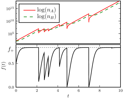
Figure 1: Typical trajectory of the system. Top: time evolution of the populations $n_{A}$ and $n_{B}$ (semi-log scale). Bottom: Corresponding time evolution of the fitness $f(t)$ (the fraction of cells in the $A$ state). Parameters are: $(\gamma_{A},\gamma_{B},k_{A},k_{B},f^{*},\beta_{0},\alpha)=(6,1,1,1,0.25,1,-0.75)$.

II.2 Catastrophes

The catastrophes in our model have two characteristics: the rate at which they happen and their strength (i.e. how many microbes are killed). The rate at which catastrophes occur, or their probability per unit time, is defined by a feedback function $\beta(f)$, which we take to depend only on the fitness of the population and not on the absolute population size (we shall return to this assumption in the Discussion). The function $\beta(f)$ characterises the response of the environment to the growth of the population. When $\beta=0$, there are no catastrophes and the fitness will reach the plateau value $f_{+}$ and stay there for ever. Nonzero constant values of $\beta$ correspond to a non-responsive environment in which the catastrophes follow Poisson statistics. We shall consider the case of a responsive environment characterised by a response function $\beta(f)$ which depends on the population fitness. In particular, we consider a nonlinear response function that has a sigmoid shape. Thus, the probability per unit time of a catastrophe is very low when the population fitness is low, but increases significantly if the fitness exceeds some threshold value. This scenario might correspond to a detection threshold in the environment’s sensitivity to population growth.

The precise environmental response function that we consider is the following:

$$\beta_{\lambda}(f)=\frac{\xi}{2}\left(1+\frac{f-f^{*}}{\sqrt{\lambda^{2}+(f-f^{*})^{2}}}\right)\,\,.$$ (6)

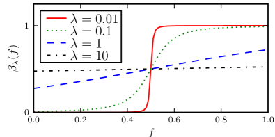
Figure 2: The response function $\beta_{\lambda}(f)$, plotted for different values of $\lambda$, with $\xi=1$ and $f^{*}=1/2$.

Although this function is defined for all $-\infty<f<\infty$, the relevant interval for the fitness is $0<f<1$. Typical shapes for this function are shown in Fig.2. The parameter $\xi$ is the asymptotic value of $\beta_{\lambda}$ when $f$ is large, and we refer to $\xi$ as the saturated catastrophe rate. As the population fitness $f$ increases, $\beta_{\lambda}$ increases from 0 to $\xi$ around the threshold value $f^{*}$ at which $\beta_{\lambda}=\xi/2$. Finally, the parameter $\lambda$ determines the sharpness of the threshold. For small values of $\lambda$ the function $\beta_{\lambda}(f)$ approaches a step function

$$\beta_{0}(f)=\xi\Theta(f-f^{*})\,\,.$$ (7)

As $\lambda$ increases, the function broadens and becomes linear over a range of $f$ near $f^{*}$:

$$\beta_{\lambda}\simeq\frac{\xi}{2}\left(1+\frac{(f-f^{*})}{\lambda}+{\mathcal{O}}\left(\frac{1}{\lambda^{2}}\right)\right)\,\,.$$ (8)

while when the parameter $\lambda$ becomes very large ($\lambda\to\infty$), $\beta_{\lambda}(f)$ becomes constant (independent of $f$) so that the catastrophes become a standard Poisson process with parameter $\xi/2$:

$$\beta_{\infty}(f)=\xi/2\,\,.$$ (9)

We emphasise that we have chosen this particular sigmoid function (6) as the $\lambda$ parameter allows a convenient tuning of its shape and thus the degree of environmental responsiveness. However, our conclusions are not affected by the particular choice of sigmoid function.

We now turn to the function describing the catastrophe strength, $\nu(n_{A}^{\prime}|n_{A})$. This is the probability that, given that $n_{A}$ cells of type $A$ are present before the catastrophe, $n_{A}^{\prime}$ will remain after the catastrophe. In order to retain our description of the model in terms of the population fitness, we shall consider that $\nu$ only depends on $n_{A}^{\prime}$ only through the ratio $n_{A}^{\prime}/n_{A}$. Then the normalisation of $\nu$ implies that

$$\nu(n_{A}^{\prime}|n_{A})=\frac{1}{n_{A}}{\mathcal{F}}(n_{A}^{\prime}/n_{A})$$ (10)

where $\int_{0}^{1}dx{\mathcal{F}}(x)=1$. When a catastrophe happens, the population size is reduced by a random factor sampled from the distribution ${\mathcal{F}}$ [i.e. the new size $n_{A}^{\prime}=n_{A}\times u$ where $n_{A}$ is the size before the catastrophe, and $u$ is a random number ($0\leq u<1$) sampled from the distribution ${\mathcal{F}}$]. This allows us to associate to each jump $n_{A}\to n_{A}^{\prime}$ a fitness jump $f\to f^{\prime}$, where $f^{\prime}=n_{A}^{\prime}/(n_{A}^{\prime}+n_{B})$. The size of these jumps will be distributed according to:

$$\mu(f^{\prime}|f)=\Theta\left(f-f^{\prime}\right){\mathcal{F}}\left(\frac{f^{\prime}(1-f)}{f(1-f^{\prime})}\right)\frac{1-f}{(1-f^{\prime})^{2}f}\,\,.$$ (11)

Eq.(11) can be obtained by rewriting expression (10) for $\nu(n_{A}^{\prime}|n_{A})$ as a function of $f$ and $f^{\prime}$ and including the Jacobian of the transformation.

In this paper, we shall consider the simple case where ${\mathcal{F}}(x)=(\alpha+1)x^{\alpha}$, with $\alpha>-1$. The explicit expression for $\nu(n^{\prime}|n)$ thus reads:

$$\nu(n^{\prime}|n)=\frac{(\alpha+1)}{n}\left(\frac{n^{\prime}}{n}\right)^{\alpha}\,\,,\qquad\qquad\alpha>-1\,\,.$$ (12)

This choice is made primarily in order to allow us to solve the model analytically: the choice implies that $\mu(f^{\prime}|f)$ factorises (see (13)) which then allows the integral equation for the probability flux balance (15) to be solved. Moreover, the choice of a power law distribution for $\nu(n_{A}^{\prime}|n_{A})$ is general in that allows for increasing, decreasing or flat functional forms. The function $\nu(n_{A}^{\prime}|n_{A})$ is plotted in Fig.3 for various values of $\alpha$. For negative $\alpha$ values, the distribution is biased towards far-reaching catastrophes that reduce fitness significantly. The case $\alpha=0$ corresponds to jumps sampled from a uniform distribution, whereas positive values give a distribution biased towards weaker catastrophes. The parameter $\alpha$ can therefore be used to tune the strength of the catastrophes (although in this work we shall always consider negative $\alpha$ values, corresponding to strong catastrophes).

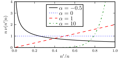
Figure 3: The jump distribution $\nu(n_{A}^{\prime}|n_{A})$, plotted for various values of $\alpha$.

We note here that with our choice for ${\mathcal{F}}(x)$ the jump distribution can be expressed as

$$\mu(f^{\prime}|f)=\Theta(f-f^{\prime})\frac{d}{df^{\prime}}\frac{m(f^{\prime})}{m(f)}\,\,.$$ (13)

where $m(0)=0$, $\int df^{\prime}\mu(f^{\prime}|f)=1$, and with,

$$m(f)=\left(\frac{f}{1-f}\right)^{1+\alpha}\,\,.$$ (14)

III Steady–state statistics

We now derive the steady-state probability distribution for the population fitness, $p(f)$. The distribution $p(f)$ must satisfy a condition of balance for the probability flux. This condition reads:

$$v(f)p(f)=\int_{f}^{f_{+}}df^{\prime}\int_{0}^{f}df^{\prime\prime}\beta(f^{\prime})p(f^{\prime})\mu(f^{\prime\prime}|f^{\prime})\,\,.$$ (15)

The left-hand side of the above equation corresponds to the deterministic probability flux due to population growth as defined in Eq.(4) [$f(t)$ increases in time as the population grows, as shown in Figure 1]. The right-hand side describes the probability flux arising from catastrophes. In this model, catastrophes always reduce the population fitness. The probability flux due to catastrophes therefore contains contributions from all possible jumps that start at some $f^{\prime}>f$ and end at some $f^{\prime\prime}<f$. These contributions must be weighted by $\beta(f^{\prime})p(f^{\prime})$: the probability of having fitness $f^{\prime}$ and undergoing a catastrophe. This balance between the fluxes due to growth and catastrophes is illustrated schematically in Figure 4.

Figure 4: Illustration of the flux balance condition. The positive probability flux due to population growth must be balanced by the negative flux due to catastrophes.

Inserting the form (13) of $\mu(f^{\prime}|f)$ in Eq.(15), the zero flux condition becomes:

$$v(f)p(f)=\int_{f}^{f_{+}}df^{\prime}\beta(f^{\prime})p(f^{\prime})\frac{m(f)}{m(f^{\prime})}\,\,.$$ (16)

We now divide the above equation by $m(f)$ and take the first derivative with respect to $f$. This yields, in terms of the function $G=vp/m$:

$$\frac{dG}{df}=-\frac{\beta G}{v}\,\,.$$ (17)

The above differential equation is then easily solved for $G$. The result for $p(f)$, using the form Eq.(14) of $m(f)$ , is finally

$$p(f)=\frac{C}{v(f)}\left(\frac{f}{1-f}\right)^{1+\alpha}\exp\left(-\int\,df\,\frac{\beta(f)}{v(f)}\right)\,\,,$$ (18)

where $C$ is a normalisation constant. The integral in Eq.(18) can be performed analytically for the model defined in the previous section. The result, which is rather cumbersome, is given in the Appendix.

We present in Fig.5 (top panel) some resulting shapes for the probability distribution $p(f)$ in the case $\lambda=0$, corresponding to a step function for the environmental response. We consider two different values of $\Delta\gamma$, in each case for $k_{A}=0$ (no switching) and a non-zero switching rate $k_{A}=k_{A}*$ defined such that $f_{+}=f^{*}$ (see section IV). In these plots we see that singularities in $p(f)$ can arise at $f=0,f^{*}$ or $f_{+}$ in different cases. In particular, the $k_{A}=0$ case produces a cusp at $f=f^{*}$ (due to the singular nature of the step function $\beta(f)$ at $f^{*}$) for small $\Delta\gamma$, and/or a divergence at $f=f_{+}$ for large $\Delta\gamma$. On the other hand $k_{A}=k_{A}*$ produces a divergence at $f_{+}=f^{*}$ in both cases.

Fig.5 (bottom panel) plots trajectories of the fitness corresponding to the parameter values of Fig.5. These trajectories reveal the interplay between two timescales: the time to relax to the plateau value $f^{*}$ in the absence of catastophes and the typical time between catastrophes. The former decreases with $\Delta\gamma$ and the latter is given by $1/\xi$ where $\xi$ is the plateau value of the response function $\beta$. A divergence of $p(f)$ at $f=f_{+}$ arises when the plateau value is typically reached before a catastrophe occurs.

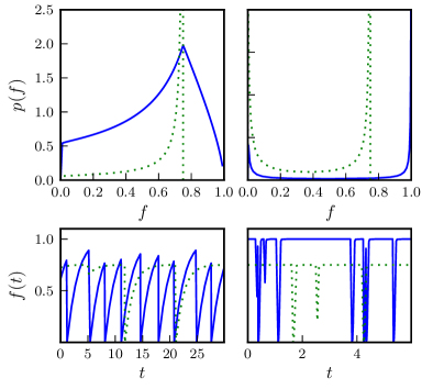
Figure 5: Top panel: Examples of steady-state fitness distribution $p(f)$ for parameter values $\Delta\gamma$= 0.1 (left) and 100 (right); other parameters are $\lambda=0$, $k_{B}=0.5$, $\xi=1$, $\alpha=-0.99$ and $f^{*}=0.75$. In each plot, the solid line corresponds to a value of $k_{A}=0$ (no switching), while the dashed plot is for $k_{A}=k_{A}^{*}$ (switching rate given by Equation 19). Bottom panel: Examples of fitness trajectories corresponding to the parameter values of the top panel.

IV Optimal strategies: to switch or not to switch?

The key question to be addressed in this work is whether random switching is advantageous to the microbial population in our model. To answer this question, we take advantage of the analytical solution (18) to investigate how the time-averaged population fitness depends on the rate $k_{A}$ of switching from the fast-growing state $A$ to the slow-growing state $B$. We are particularly interested in the effect of the parameter $\lambda$, which controls the sharpness of the environment’s response to the population.

In Fig.6 we plot the average population fitness against $k_{A}$ for several values of $\lambda$. For a non responsive environment [i.e. in the limit of large $\lambda$, where the catastrophe rate takes the constant non-zero value $\xi/2$ (9)], the population fitness has only one (boundary) maximum for switching rate $k_{A}\to 0$. This means that the optimal rate of population growth is achieved when the bacteria do not switch away from the fittest state $A$. It should be noted that we consider the limit $k_{A}\to 0$, so that the population always contains some small residual fraction in the unfit $B$ state, which becomes a finite fraction of the population after a catastrophe. Subsequently, in between the catastrophes, the $A$ subpopulation grows quickly to dominate the population and the fitness evolves towards the value $f_{+}=1$, which follows from Eq.(5) when $k_{A}=0$.

In contrast, as the environment is made responsive by decreasing the parameter $\lambda$, a local maximum appears in the population fitness, for nonzero switching rate $k_{A}$. This implies that for responsive environments, switching into the slow-growing state represents an optimal strategy for the microbes. The height of the peak at $k_{A}\neq 0$ can surpass that of the peak at $k_{A}=0$, showing that random switching can be advantageous compared to keeping the whole population in the fast-growing state, if the environment is responsive. Thus the two maxima correspond to two alternative strategies which we term switching for the peak at $k_{A}=k_{A}^{*}$ and non-switching for the peak at $k_{A}=0$.

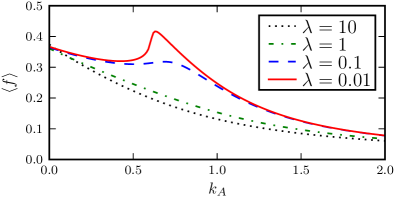
Figure 6: Average population fitness $\left\langle f\right\rangle$ as a function of the $A\to B$ switching rate $k_{A}$, for several values of parameter $\lambda$. For large values of $\lambda$ the average fitness peaks for zero switching, $k_{A}=0$. However, as $\lambda$ decreases, a second peak arise at non zero $k_{A}$, indicating that random switching can be a favourable strategy when the environment is responsive. Parameters values are: $k_{B}=0.1$, $\Delta\gamma=1$, $\alpha=-0.99$, $\xi=1$ and $f^{*}=0.5$.

To gain further insight into the meaning of these two strategies, and to determine which circumstances favour one strategy over the other, we focus on the limiting case $\lambda=0$, where the response function is a step function with its threshold at $f=f^{*}$. We assume that the environmental threshold $f^{*}$ is less than the maximum population fitness $f_{+}$. (If this is not the case, the unrealistic situation arises where the population never has a high enough fraction of $A$ cells to trigger any catastrophes.) Since $f_{+}$ depends on the switching rate $k_{A}$ via Eq.(5), this condition $f^{*}<f_{+}$ implies a maximum value $k_{A}^{*}$ for $k_{A}$:

$$k_{A}^{*}=\frac{(1-f^{*})(\Delta\gamma\,f^{*}+k_{B})}{f^{*}}\,\,.$$ (19)

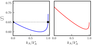
Figure 7: Average population fitness $\left\langle f\right\rangle$ as a function of $k_{A}$ for a threshold response function. The left plot is an instance where the maximal fitness occurs at non-zero $k_{A}$, while the right plot shows an example where the maximum fitness occurs at $k_{A}=0$. In both plots parameters are $\alpha=-0.99$, $f^{*}=0.75$, $\beta_{0}=1$ and $k_{B}=0.8$; $\Delta\gamma=1$ (left) and $\Delta\gamma=4$ (right).

Fig.7 shows two examples of how the average fitness $\left\langle f\right\rangle$ depends on $k_{A}$ in the range 0 to $k_{A}^{*}$. One can see that there are always two boundary maxima located at $k_{A}=0$ and at $k_{A}=k_{A}^{*}$; these correspond to the non-switching and switching strategies.

We plot in Fig.8 typical trajectories of the population fitness for the two cases corresponding to the black circles in Fig.7 (left panel). These trajectories have the same time-averaged population fitness, but they show very different dynamical behaviour. The non-switching strategy ($k_{A}=0$) is characterised by a fast evolution of the fitness towards its maximum $f_{+}=1$. However this triggers frequent catastrophes which cause sudden decreases in fitness. In contrast, for the switching strategy ($k_{A}\to k_{A}^{*}$), the fitness has a slower growth towards a plateau value at the detection threshold $f^{*}$. In this way, the population reduces the frequency of catastrophes by maintaining itself in a heterogeneous state with a non-zero fraction of slower-growing cells which do not trigger catastrophes.

We next consider how the parameters of our model affect the balance between the switching and non-switching strategies. To this end, we plot “phase diagrams” showing which of these two strategies achieves a higher population growth rate for a given set of parameters. Figure 9 considers the parameters describing the microbial population: the difference $\Delta\gamma$ in growth rate between the $A$ and $B$ states and the switching rate $k_{B}$ from the slow-growing $B$ state to the fast-growing $A$ state. This diagram shows that the switching strategy is only favourable when the $B$ state does not carry too high a cost in terms of growth rate ($\Delta\gamma$ not too large) and when switching to the $B$ state is unlikely to be immediately followed by a reverse switch back into the $A$ state ($k_{B}$ not too large). In Fig.10 we consider instead the parameters describing the environmental response: the detection threshold $f^{*}$ and the saturated catastrophe rate $\xi$. Here, we see that the switching strategy (i.e. attempting to avoid catastrophes) is favoured when the saturated catastrophe rate $\xi$ is high or when the threshold value $f^{*}$ is high (since for high thresholds the population does not have to pay a very high price in terms of $B$ cells to avoid triggering catastrophes). For very low detection thresholds $f^{*}$, lower than typical values of the fitness, the environmental response will almost always “detect” the population, and the environmental behaviour will thus be similar to the situation of a non–responsive environment, which corresponds to the limiting case where $f^{*}=0$. In this case, as discussed earlier, non-switching is the optimal strategy. Figure 10 also demonstrates the effect of changing the catastrophe strength parameter $\alpha$ (dashed and dotted lines). The switching strategy is favoured by strong catastrophes (negative $\alpha$), while the non-switching strategy is more likely to be optimal for weak catastrophes (i.e. larger positive $\alpha$). All this points to the conclusion that in general, switching tends to be an advantageous strategy when the characteristics of the catastrophic environment are particularly adverse (large $\xi$ and negative $\alpha$) and when the detection threshold is not too low.

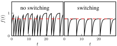
Figure 8: Two typical trajectories illustrating the two possible strategies: in the left panel, the switching rate $k_{A}=0$, the fitness evolves towards its maximal value $f=1$ but many catastrophes are induced; in the right panel $k_{A}$ is set to a value smaller but very close to $k_{A}^{*}$ ($k_{A}=0.6155=0.997k_{A}^{*}$), the fitness evolves to just above the threshold value with relatively few catastrophes induced. These strategies correspond to the two black points in the top left plot of Fig.7. The value of $f^{*}$ is 0.75, as indicated by the red dashed line, and the average fitness is the same in both plots ($\left\langle f\right\rangle=0.652585$).

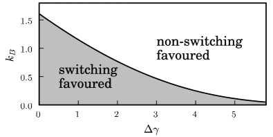
Figure 9: “Phase diagram” showing the optimal strategy as a function of the parameters $k_{B}$ and $\Delta\gamma$ which describe the microbial population. In the shaded area switching is the optimal strategy, while in the unshaded area, the non-switching strategy leads to a larger average population fitness. The other parameters are: $\alpha=-0.99$, $f^{*}=0.75$, $\xi=1$.

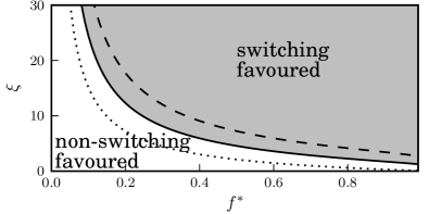
Figure 10: “Phase diagram” showing the optimal strategy as a function of the parameters $\xi$ and $f^{*}$ which describe the environmental response. In the shaded area switching is the optimal strategy, while in the unshaded area, the non-switching strategy leads to a larger average population fitness. The other parameters are $\Delta\gamma=1$ and $k_{B}=1$. The black solid line shows the “phase boundary” for $\alpha=-0.5$, while the dotted and dashed line correspond to $\alpha=-0.99$ and $\alpha=0$.

V Discussion and further directions

In this work we have considered the possible advantages of phase variation (random switching between phenotypic states) for a microbial population in a catastrophic responsive environment. To this end, we solved analytically for the steady-state statistics of a model which includes two microbial sub-populations that grow and switch, and a single environment which occasionally mounts catastrophic attacks on the microbial population. Importantly, the model includes feedback between the state of the population and the frequency of catastrophic events via an environment response function which depends on the population through its fitness i.e. the instantaneous rate of growth. Our results show that, when the environment is responsive to the population, switching can increase the average fitness (i.e. growth rate) of the population. A general picture emerges from our work of two competing strategies for dealing with a catastrophic responsive environment: not switching and thus maximising the instantaneous growth rate regardless of catastrophes versus using switching to tune the population to reduce the likelihood of catastrophes.

An important feature of this work is the fact that we are able to solve the model analytically, leading to an explicit formula for the population fitness as a function of the model parameters. To achieve this analytical result, we make a number of assumptions, the most important being that the environmental feedback depends on the instantaneous growth rate rather than on the population size. Although this is a rather idealized assumption, microbe-host interactions are in reality likely to be sensitive to microbial growth rate [25], since several intracellular small molecules and proteins, including ppGpp, cAMP and H-NS, whose concentrations are growth-rate dependent [26, 27], have been shown to regulate microbial virulence factors [28, 29, 30].

The main conclusion of our work is that phase variation can provide a mechanism by which a microbial population can tune its composition so as to minimize the likely environmental response, thus increasing its average growth rate (or average fitness). The model thus provides an alternative scenario for the role of phase variation to those proposed in other theoretical studies, which we now take the opportunity to review briefly.

Various works have considered models in which the environment flips randomly or periodically between several different states, each favouring a particular cell phenotype. These models do not include feedback between the population and the environmental flipping rate. For the case of two environmental states and two cellular phenotypes, Lachmann and Jablonka [12] considered a discrete time model with a periodic environment, while Ishii et al [13] addressed a similar problem but explicitly looked for the evolutionary stable state. Thattai and Van Oudenaarden [14] also considered the two-environment, two-phenotype case, using a continuous time model with Poissonian switching of the environment, while a detailed analytical treatment of this case was presented by Gander et al. [15] and a simulation study was carried out by Ribeiro [16] with a more detailed model of the phenotypic switching mechanism, while Wolf et al. [17] simulated a model that also included environmental sensing. These studies showed that the total growth rate of the population can be enhanced by phenotypic switching (compared to no switching), for some parameter regimes, and that the optimum switching rate is tuned to the environmental flipping rate. A similar model, but aimed specifically at the case of the persister phenotype, in which cells grow very slowly but are resistant to antibiotics [20], was considered by Kussell et al. for a periodic environment [21]. In this model, the growth rate of the non-persister phenotype is negative (signifying population decrease) in the “antibiotic” environment.

Several other studies have considered random switching from a different context: as a means to avoid the need for sensing and responding to environmental changes, in the case that environmental sensing is inaccurate, faulty or expensive. In this context, Kussell and Leibler [18] considered theoretically a model with many environments and many cellular states, where a cost is attached to sensing environmental changes, while Wolf et al. [17] simulated a two state-two environment model where sensing was subject to a variety of possible defects. Both these studies concluded that random switching can be a good strategy to overcome disadvantages associated with environmental sensing.

In a somewhat different approach, Wolf et al. [31] used simulations to study a two state-two environment model in which the growth rate of the $A$ and $B$ states is frequency dependent—i.e. a given microbial sub-population grows faster when its abundance is low. Such “frequency-dependent selection” is well known to promote population heterogeneity; however, Wolf et al. did not find any advantages for reversible switching as a means to generate this heterogeneity as opposed to terminal cellular differentiation. In a sense, the model presented in this paper also incorporates frequency dependent selection, since catastrophes are less likely when the $A$ sub-population is small. However, in contrast to Wolf et al., we find that reversible switching does play an important role. If switching in our model were not reversible, there would be no way for the fast-growing $A$ subpopulation to regenerate from the surviving $B$ cells after a catastrophe.

Although the majority of theoretical work in this area, including that presented in this paper, has focused on the interplay between cellular switching and environmental changes, this is not the only perspective from which the role of phase variation can be viewed. For example, an alternative scenario, which does not require a changing environment, was recently presented by Ackermann et al. [32]. These authors showed that random switching into a “self-sacrificing” phenotypic state can be evolutionarily favoured if the individuals in that state have on average greater access to some beneficial resource. This idea raises a number of interesting questions which we hope to pursue in future research.

Finally we note that the theoretical framework developed in the present work, although applied here to the case of detrimental and instantaneous catastrophes, could also be used to model environmental changes more generally. For example, in the symmetric two state-two environment model considered by Thattai and van Oudenaarden [14], the environment flips randomly between two states and these flips are accompanied by a change in fitness from $f$ to $1-f$. This could be incorporated in our theoretical framework by setting the $\beta(f)$ to a constant value and the jump distribution $\mu(f|f^{\prime})$ to:

$$\mu(f^{\prime}|f)=\delta\left(f^{\prime}-(1-f)\right)\,\,.$$ (20)

However, such a choice of $\mu(f|f^{\prime})$ would result in fundamentally different conclusions to those of the present study, because the fitness in the Thattai-van Oudenaarden model (and in other similar models) is not necessarily decreased when the environment changes. In fact, if a large fraction of the cells are in the slow-growing state before the environment flips so that $f<1/2$, then the environmental change will actually increase the fitness of the population. In contrast, in the present work, all catastrophes are detrimental and the advantage of switching lies in avoiding the triggering of an environmental response.

The present study suggests a number of avenues for further work. First, it would be useful to check the robustness of the results to changes in the choice of catastrophe distributions. Here we have adopted the power law (12) which allows the exact solution of the model and generates a broad range of catastrophes sizes. Such a distribution could be justified in the context of an ‘antibiotic’ environment, as representing the dose-response variability of antimicrobes [33] and variability in the dosage. One could also explore other distributions such as exponentially distributed catastrophes or those centred about some particular catastrophe fraction $f^{\prime}=af$ with $a<1$. It remains to be determined which choice is most biologically relevant in different contexts.

Another point which also deserves investigation in future work is the relation between the choice of switching strategy and the variability in the population fitness. For example in Fig.5 one can see that the different strategies give very different widths for the fitness distribution $p(f)$. In this work we defined the optimal strategy as that which gives the maximal average growth of the population. However, it might also be relevant to include fitness fluctuations in the criteria for optimality.

It is also important to consider the case where the environmental response depends on the absolute size of a particular subpopulation. Here, we expect that the population size may reach a steady state governed by the balance between growth and catastrophes. The total population size could then be maximised either by maximising the growth rate, regardless of catastrophes, or by tuning the population composition to avoid triggering catastrophes. We thus expect that the two strategies identified in the present work will prove to be relevant to a variety of models. Moreover, we note that the distinction between models based on growth rate and those based on population size may vanish for scenarios with constant population size such as chemostat cultures [34]. Equally interesting are the prospects for including spatial effects, such as adhesion to host surfaces, or transfer between different environmental compartments, in the model, and for generalising the model to include many different microbial states, in which case the same theoretical framework could perhaps be used to describe genetic evolution of microbial populations in catastrophic responsive environments.

Appendix A Explicit form of $p(f)$

Below we give the explicit form for the integral appearing in (18) when $\beta(f)$ is given by (6):

$$\int df\,\frac{\beta(f)}{v(f)}=\frac{\xi}{2\Delta\gamma\Delta f}\log\left\{\frac{(f-f_{-})}{(f_{+}-f)}\left[\frac{2\Delta f((f^{*}-f)(f^{*}-f_{-})+\lambda^{2}+g(f,f^{*})g(f_{-},f^{*}))}{(f-f_{-})(f^{*}-f_{-})g(f_{-},f^{*})}\right]^{\frac{(f^{*}-f_{-})}{g(f_{-},f^{*})}}\right.\\ \times\left.\left[\frac{2\Delta f((f-f^{*})(f_{+}-f^{*})+\lambda^{2}+g(f,f^{*})g(f_{+},f^{*})}{(f_{+}-f)(f_{+}-f^{*})g(f_{+},f^{*})}\right]^{\frac{(f_{+}-f^{*})}{g(f_{+},f^{*})}}\right\}\,\,,$$ (21)

where

$$g(a,b)=\sqrt{(a-b)^{2}+\lambda^{2}}\,\,.$$ (22)

From this result, the explicit expression for the fitness distribution function $p(f)$ can be easily derived.

References

- [1] M. W. van der Woude and A. Bäumler, Clin. Microbiol. Reviews 17, 581 (2004).
- [2] M. W. van der Woude, FEMS Microbiol. Lett. 254, 190 (2006).
- [3] I. R. Henderson, P. Owen, and J. P. Nataro, Mol. Microbiol. 33, 919 (1999).
- [4] P. Visco, R. J. Allen, and M. R. Evans, Phys. Rev. Lett. 101, 118104 (2008).
- [5] P. Visco, R. J. Allen, and M. R. Evans, Phys. Rev. E 79, 031923 (2009).
- [6] M. Ptashne, A Genetic Switch, Phage and Higher Organisms, 2nd ed. (Blackwell, Cambridge, USA, 1992).
- [7] A. Novick and M. Weiner, Proc. Natl. Acad. Sci. U. S. A. 43, 553 (1957).
- [8] T. A. Carrier and J. D. Keasling, J. Theor. Biol. 201, 25 (1999).
- [9] P. B. Warren and P. R. ten Wolde, J. Phys. Chem. B 109, 6812 (2005).
- [10] B. Hallet, Curr. Opin. Microbiol. 4, 570 (2001).
- [11] J. Seger and H. Brockman, What is bet-hedging?, in Oxford Surveys in Evolutionary Biology, Oxford University Press, 1987.
- [12] M. Lachman and E. Jablonka, J. Theor. Biol. 181, 1 (1996).
- [13] K. Ishii, H. Matsuda, Y. Iwasa, and A. Sasaki, Genetics 121, 163 (1989).
- [14] M. Thattai and A. van Oudenaarden, Genetics 167, 523 (2004).
- [15] M. J. Gander, C. Mazza, and H. Rummler, J. Math. Biol. 55, 259 (2007).
- [16] A. S. Ribeiro, Phys. Rev. E 78, 061902 (2008).
- [17] D. M. Wolf, V. V. Vazirani, and A. P. Arkin, J. Theor. Biol. 234, 227 (2005).
- [18] E. Kussell and S. Leibler, Science 309, 2075 (2005).
- [19] M. Acar, J. T. Mettetal, and A. van Oudenaarden, Nature Genetics 40, 471 (2008).
- [20] N. Q. Balaban, J. Merrin, R. Chait, L. Kowalik, and S. Leibler, Science 305, 1622 (2004).
- [21] E. Kussell, R. Kishony, N. Q. Balaban, and S. Leibler, Genetics 169, 1807 (2005).
- [22] M. A. Mulvey, Cell Microbiol. 4, 257 (2002).
- [23] M. H. A. Davis, J. R. Statist. Soc. B 46, 353 (1984).
- [24] O. Pulkkinen and J. Berg, arXiv:0807.3521 (2008).
- [25] A. K. Johri, V. Patwardhan, and L. C. Paoletti, Can. J. Microbiol. 51, 283 (2005).
- [26] T. Ferenci, Adv. Microb. Physiol. 53, 169 (2008).
- [27] M. Schaechter, J. L. Ingraham, and F. C. Neidhardt, Microbe (ASM Press, Washington, DC, USA, 2006).
- [28] J. Pizarro-Cerdá and K. Tedin, Mol. Microbiol. 52, 1827 (2004).
- [29] C. Pesavento and R. Hengge, Curr. Opin. Microbiol. 12, 170 (2009).
- [30] O. Schröder and R. Wagner, Biol. Chem. 383, 945 (2002).
- [31] D. M. Wolf, V. V. Vazirani, and A. P. Arkin, J. Theor. Biol. 234, 255 (2005).
- [32] M. Ackermann et al., Nature 454, 987 (2008).
- [33] C. H. Nightingale, P. G. Ambrose, and G. L. Drusano, Antimicrobial Pharmacodynamics in Theory and Clinical Practice, 2nd ed. (Informa Healthcare, New York, USA, 2007).
- [34] J. L. Ingraham, O. Maaloe, and F. C. Neidhardt, Growth of the Bacterial Cell (Sinauer Associates Inc, 1983).