Fluctuation-Induced Interaction between Randomly Charged Dielectrics

Abstract

Monopolar charge disorder effects are studied in the context of fluctuation-induced interactions between neutral dielectric slabs. It is shown that quenched bulk charge disorder gives rise to an additive contribution to the net interaction force which decays as the inverse distance between the slabs and may thus completely mask the standard Casimir–van der Waals force at large separations. By contrast, annealed (bulk or surface) charge disorder leads to a net interaction force whose large-distance behavior coincides with the universal Casimir force between perfect conductors, which scales as inverse cubic distance, and the dielectric properties enter only in subleading corrections.

Recent ultrahigh sensitivity experiments on Casimir (zero temperature and ideally polarizable surfaces) and van der Waals (finite temperature and non-ideally polarizable surfaces) interactions between surfaces in vacuo bordag ; kim have highlighted the need for an accurate assessment of the possible electrostatic contribution to the total interaction when the surfaces bear a disordered charge distribution speake . The surface charge distribution can have various origins. In the so-called patch effect, the variation of the local crystallographic axes of the exposed surface of a clean polycrystalline sample can lead to a variation of the local surface potential barrett . These variations are of course sample specific and depend heavily on the method of preparation of the samples. The electrostatic forces due to this surface potential disorder cannot be eliminated by grounding the two interacting surfaces. A similar type of surface charge disorder can also be expected for amorphous films deposited on crystalline substrates. Surface annealing of these films can produce a grain structure of an extent that can be larger than the thickness of the deposited surface film liu . In addition, adsorption of various contaminants can also influence the nature and type of the surface charge disorder.

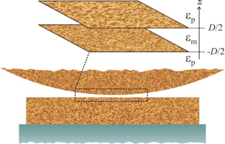
Figure 1: (Color online) A typical experimental set up (bottom) is modeled with a plane-parallel system (top) of two dielectric slabs (half-spaces) of dielectric constant $\varepsilon_{p}$ interacting across a medium of dielectric constant $\varepsilon_{m}$. The charge distribution in the bulk of the slabs and on the two bounding surfaces at $z=\pm D/2$ has a disordered component (shown schematically by small light and dark patches) with zero mean but finite variance, and may be either quenched or annealed in nature.

Here we assess the effect of various types of monopolar charge disorder on the interaction between two macroscopic surfaces, delimiting two semi-infinite net-neutral dielectric slabs, separated by a layer of vacuum or an arbitrary dielectric material (Fig. 1). Since the nature and distribution of the charge disorder in any of the experiments is in general not known, we consider different a priori models for the distribution of disorder. Specifically, we assume that the charge disorder originates from randomly distributed monopolar charges which may be present both in the bulk and on the bounding surfaces and can be either annealed or quenched. It turns out that the type and the nature of the disorder has important consequences for the total interaction between apposed bodies and can even dominate or give a contribution comparable to the underlying Casimir–van der Waals (vdW) effect. Our main goal is thus to investigate the interaction fingerprint of the charge disorder and to compare its contribution to the total interaction with the zero-frequency Casimir–vdW interaction between macroscopic surfaces. This may in turn help in assessing whether the experimentally observed interactions can be interpreted in terms of disorder-induced effects or pure Casimir–vdW interactions.

We consider two semi-infinite slabs of dielectric constant $\varepsilon_{p}$ and temperature $T$ with parallel planar inner surfaces (of infinite area $S$) located normal to the $z$ axis at $z=\pm D/2$, where $D$ is thus the distance between their surfaces (see Fig. 1). The inner gap is filled with a material of dielectric constant $\varepsilon_{m}$. We shall assume that the dielectric slabs have a disordered monopolar charge distribution, $\rho(\mathbf{r})$, which may arise from charges residing on bounding surfaces [$\rho_{s}(\mathbf{r})$] and/or in the bulk [$\rho_{b}(\mathbf{r})$], i.e. $\rho(\mathbf{r})=\rho_{s}(\mathbf{r})+\rho_{b}(\mathbf{r})$. The charge disorder will be taken to be of zero mean (i.e., the slabs are net neutral) and Gaussian-distributed note0 with no correlation in space i.e., $\langle\!\langle\rho({\bf r})\rho({\bf r}^{\prime})\rangle\!\rangle=g(\mathbf{r})\delta({\bf r}-{\bf r}^{\prime})$ [where $\langle\!\langle\cdots\rangle\!\rangle$ denotes the disorder average]. The total correlation is the sum of the surface and bulk correlations $g(\mathbf{r})=g_{s}(\mathbf{r})+g_{b}(\mathbf{r})$. For the slab geometry considered here, the charge distribution is assumed to be statistically invariant in the plane of the dielectrics but with a variance dependent on $z$ as

$$g_{s}(\mathbf{r}) = g_{s}e_{0}^{2}[\delta(z+D/2)+\delta(z-D/2)],$$ (1)

$$g_{b}(\mathbf{r}) = \left\{\begin{array}[]{ll}g_{b}e_{0}^{2}&\quad|z|>D/2,\\ 0&\quad|z|<D/2,\end{array}\right.$$ (4)

where $e_{0}$ is the elementary charge. It is worth mentioning how this sort of disorder distribution might arise. If the bulk material has charge impurities at the sites ${\mathbf{r}}_{i}$ distributed uniformly and independently with density $n_{b}$ and charges $q_{i}=\pm q_{b}e_{0}$ with equal probability, then we clearly have $\rho_{b}({\bf r})=\sum_{i}q_{i}\delta({\bf r}-{\bf r}_{i})$ and find $\langle\!\langle\rho_{b}({\bf r})\rangle\!\rangle=0$ and $\langle\!\langle\rho_{b}({\bf r})\rho_{b}({\bf r})\rangle\!\rangle=q_{b}^{2}e_{0}^{2}n_{b}\delta({\bf r}-{\bf r}^{\prime})$. We can thus make the correspondence $g_{b}=q_{b}^{2}n_{b}$. Similarly, one can make the correspondence $g_{s}=q_{s}^{2}n_{s}$ with $n_{s}$ being the surface density of impurity charges $\pm q_{s}$ on bounding surfaces.

The partition function for the classical Casimir–vdW interaction (the zero-frequency Matsubara modes of the electromagnetic field) may be written as a functional integral over the scalar field $\phi(\mathbf{r})$,

$${\mathcal{Z}}[\rho(\mathbf{r})]=\int[{\mathcal{D}}\phi(\mathbf{r})]\,\,e^{-\beta{\mathcal{S}}[\phi(\mathbf{r});\rho(\mathbf{r})]},$$ (5)

with $\beta=1/k_{\mathrm{B}}T$ and the effective action

$${\mathcal{S}}[\phi(\mathbf{r});\rho(\mathbf{r})]=\int{\mathrm{d}}\mathbf{r}\,\big{[}{\textstyle{\frac{1}{2}}}\varepsilon_{0}\varepsilon({\mathbf{r}})\,(\nabla\phi(\mathbf{r}))^{2}+{\mathrm{i}}\,\rho(\mathbf{r})\phi(\mathbf{r})\big{]},$$ (6)

where $\varepsilon({\mathbf{r}})=\varepsilon_{p}$ for $|z|>D/2$ and $\varepsilon_{m}$ otherwise. In order to evaluate the averaged quantities such as the effective interaction, one needs to average the partition function over different realizations of the disordered charge distribution, $\rho(\mathbf{r})$ ali-rudi . It is thus important to distinguish between quenched and annealed disorder that involve different averaging schemes. For quenched disorder, the disorder charges are frozen and cannot fluctuate; for annealed disorder the charges can fluctuate and, in particular, the charge distribution in the two slabs can adapt itself to minimize the free energy of the system. These two different disorder types lead to very different physical behaviors as will be demonstrated below.

Let us first consider the quenched disorder model, where one must take the disorder average over the sample free energy, $\ln{\mathcal{Z}}[\rho(\mathbf{r})]$, in order to calculate the averaged quantities. The free energy of the quenched system,

$$\beta{\mathcal{F}}_{\mathrm{quenched}}=-\langle\!\langle\ln{\mathcal{Z}}[\rho(\mathbf{r})]\rangle\!\rangle,$$ (7)

may be calculated from Eq. (5) as

$$\beta{\mathcal{F}}_{\mathrm{quenched}}={\frac{1}{2}}{\mathrm{Tr}}\ln G^{-1}({\mathbf{r}},{\mathbf{r}}^{\prime})+{\frac{\beta}{2}}{\mathrm{Tr}}\big{\{}g({\mathbf{r}})G({\mathbf{r}},{\mathbf{r}}^{\prime})\big{\}},$$ (8)

where $G({\mathbf{r}},{\mathbf{r}}^{\prime})$ is the Green’s function defined via

$$\varepsilon_{0}\nabla\cdot[\varepsilon(\mathbf{r})\nabla G(\mathbf{r},\mathbf{r}^{\prime})]=-\delta(\mathbf{r}-\mathbf{r}^{\prime}).$$ (9)

In the first term of Eq. (8), we recognize the standard zero-frequency vdW interaction $\beta{\mathcal{F}}_{\mathrm{vdW}}\equiv{\textstyle{\frac{1}{2}}}{\mathrm{Tr}}\ln G^{-1}({\mathbf{r}},{\mathbf{r}}^{\prime})$. The second term, $\beta{\mathcal{F}}_{g}\equiv{\textstyle{\frac{\beta}{2}}}{\mathrm{Tr}}\{g({\mathbf{r}})G({\mathbf{r}},{\mathbf{r}}^{\prime})\}$, represents the contribution of the quenched charge disorder, which turns out to be additive in the free energy.

Figure 2: a) Ratio of the total force (13) to the zero-frequency vdW force (11) between net-neutral dielectric half-spaces (in vacuum, $\varepsilon_{m}=1$) bearing quenched monopolar charge disorder for fixed bulk and surface disorder variances $g_{b}=5\times 10^{-8}\,{\mathrm{nm}}^{-3}$, $g_{s}=\sqrt[3]{g_{b}^{2}}$ and different dielectric constants $\varepsilon_{p}=2,5,10,20,40,80,100$ (dashed curves from top). b) Magnitude of the rescaled total force (13) in the quenched case as a function of the rescaled distance for fixed $\varepsilon_{p}=10$, $g_{s}=0$ and various bulk disorder variances $g_{b}=10^{-6},10^{-7},10^{-8},10^{-9},10^{-10},10^{-11}\,{\mathrm{nm}}^{-3}$ (dashed curves from top). Solid curve is the pure vdW force (11). Inset is the ratio of the total force to the vdW force (11) for the same range of $D$. c) is the same as (b) but for annealed disorder (top panel, from Eq. (18)). Annealed curves stay close to one another and are bracketed by the perfect conductor result (Eq. (22), top solid line, labeled by $\zeta(3)$) for large disorder and the vdW result for no disorder (Eq. (11), bottom solid line, labeled by ${\mathrm{Li}}_{3}(\Delta^{2})$) as seen more clearly from the force ratio shown in the bottom panel. (b) and (c) are plotted in log-log scale.

The quenched expression (8) is valid for any arbitrary disorder variance $g({\mathbf{r}})$. We now particularize to the case of planar dielectrics by using Eqs. (1) and (4), in which case the zero-frequency vdW contribution per unit area,

$$\frac{\beta{\mathcal{F}}_{\mathrm{vdW}}}{S}={\frac{1}{2}}\!\int\!\!\frac{{\mathrm{d}}^{2}Q}{(2\pi)^{2}}\ln{(1-\Delta^{2}\,e^{-2QD})},$$ (10)

yields the standard vdW force, $f_{\mathrm{vdW}}=-\partial{\mathcal{F}}_{\mathrm{vdW}}/\partial D$, as

$$\frac{\beta f_{\mathrm{vdW}}}{S}=-\frac{{\mathrm{Li}}_{3}(\Delta^{2})}{8\pi D^{3}}.$$ (11)

The dielectric jump parameter is defined as $\Delta=(\varepsilon_{p}-\varepsilon_{m})/(\varepsilon_{p}+\varepsilon_{m})$ and $\mathrm{Li_{3}}(\cdot)$ is the trilogarithm function. The bulk and surface disorder contributions are obtained as

$$\frac{\beta{\mathcal{F}}_{g}}{S} = -\frac{2g_{b}l_{\mathrm{B}}\varepsilon_{m}\Delta}{(\varepsilon_{m}+\varepsilon_{p})^{2}}\int_{0}^{\infty}\frac{{\mathrm{d}}Q}{Q}\frac{e^{-2QD}}{1-\Delta^{2}e^{-2QD}}$$ (12)

$$-\bigg{(}\frac{2g_{s}l_{\mathrm{B}}\varepsilon_{m}|\ln(1-\Delta^{2})|}{(\varepsilon_{m}+\varepsilon_{p})^{2}\Delta}\bigg{)}\frac{1}{D},$$

at all separations $D$ with $l_{\mathrm{B}}=\beta e_{0}^{2}/(4\pi\varepsilon_{0})\simeq 56.8$ nm being the Bjerrum length in vacuum at room temperature ($T=300\,{\mathrm{K}}$). The quenched contribution from the bulk disorder (first term) in Eq. (12) is in principle infra-red divergent, however the corresponding force is finite. The total force, $f_{\mathrm{quenched}}=-\partial{\mathcal{F}}_{\mathrm{quenched}}/\partial D$, thus follows as

$$\frac{\beta f_{\mathrm{quenched}}}{S}=-\frac{g_{b}l_{\mathrm{B}}\Delta}{2\varepsilon_{p}D}-\bigg{(}\frac{2g_{s}l_{\mathrm{B}}\varepsilon_{m}|\ln(1-\Delta^{2})|}{(\varepsilon_{m}+\varepsilon_{p})^{2}\Delta}\bigg{)}\frac{1}{D^{2}}-\frac{{\mathrm{Li}}_{3}(\Delta^{2})}{8\pi D^{3}}.$$ (13)

Here we obtain a sequence of scaling behaviors of different origins: a leading $1/D$ term due to the quenched bulk disorder, a subleading $1/D^{2}$ term from the surface charge disorder, and the pure vdW term that goes as $1/D^{3}$ and prevails in the absence of charge disorder. The disorder contributions (first and second terms in Eq. (13)) are attractive when the dielectric mismatch $\Delta>0$ (e.g., for two dielectrics slabs in vacuum) and repulsive otherwise (e.g., for the two surfaces of a single slab in vacuum). One might expect that globally electroneutral slabs would exhibit a dipolar-like interaction force on the leading order rather than the monopolar forms $1/D$ (or $1/D^{2}$) obtained for the bulk (or surface) charge distribution. The physics involved is indeed subtle as the disorder terms result from the self-interaction of the charges with their images (which follows from $G({\mathbf{r}},{\mathbf{r}})$, Eq. (8), and only in a dielectrically inhomogeneous system) and not from dipolar interactions (which come from an expansion of $G({\mathbf{r}},{\mathbf{r}}^{\prime})$ when $|{\mathbf{r}}-{\mathbf{r}}^{\prime}|$ is large). Statistically speaking each charge on average (as any other charge has an equal probability of being of the same or opposite sign) only sees its image, thus explaining the leading monopolar form in the net force.

The remarkable result is however the relative importance of the disorder-induced forces, which exhibit a much weaker decay with the separation, $D$. They may thus completely mask the standard Casimir–vdW force at sufficiently large separations depending on the dielectric constants and the disorder variances as shown in Figs. 2a and 2b; the bulk disorder variance is chosen here within the typical range $g_{b}\simeq 10^{-11}-10^{-6}\,{\mathrm{nm}}^{-3}$ (corresponding to impurity charge densities of $10^{10}-10^{15}\,e_{0}/{\mathrm{cm}}^{3}$) Kao_Pitaevskii .

For relatively small surface disorder ($g_{s}\ll g_{b}l_{\mathrm{B}}$), the anomalous $1/D$ behavior is predicted to dominate the vdW $1/D^{3}$ behavior beyond the crossover distance

$$D_{b}=\left[\frac{\varepsilon_{p}{\mathrm{Li}}_{3}(\Delta^{2})}{4\pi g_{b}l_{\mathrm{B}}\Delta}\right]^{1/2},$$ (14)

which, for typical parameter values, covers the experimentally relevant range of distances from a few hundreds of nm to several microns (Fig. 2b, main set). For strong surface disorder ($g_{s}\gg g_{b}l_{\mathrm{B}}$), on the other hand, one expects the $1/D^{2}$ behavior to dominate beyond

$$D_{s}=\frac{(\varepsilon_{m}+\varepsilon_{p})^{2}\Delta\,{\mathrm{Li}}_{3}(\Delta^{2})}{16\pi g_{s}l_{\mathrm{B}}\varepsilon_{m}|\ln(1-\Delta^{2})|}.$$ (15)

So far we have only examined the effects from the quenched disorder. In reality one may encounter disordered charges with some degree of annealing. A possible idealization is to assume that the disorder is completely annealed (the intermediate partially annealed cases are also analytically tractable as shown recently mama but will not be considered here). In the annealed disorder model, the disorder average is taken over the sample partition function, ${\mathcal{Z}}[\rho(\mathbf{r})]$; hence, the free energy of the system,

$$\beta{\mathcal{F}}_{\mathrm{annealed}}=-\ln\,\langle\!\langle{\mathcal{Z}}[\rho(\mathbf{r})]\rangle\!\rangle,$$ (16)

may be evaluated as

$$\beta{\mathcal{F}}_{\mathrm{annealed}}={\frac{1}{2}}{\mathrm{Tr}}\ln\big{[}G^{-1}({\mathbf{r}},{\mathbf{r}}^{\prime})+\beta g({\mathbf{r}})\delta({\mathbf{r}}-{\mathbf{r}}^{\prime})\big{]}.$$ (17)

Note that, unlike the quenched result in Eq. (8), the disorder and the pure Casimir–vdW contributions can not be separated in general when the disorder is annealed.

In the case of two interacting slabs with the surface and bulk disorder variances (1) and (4), the modified inverse Green’s function $G^{-1}({\mathbf{r}},{\mathbf{r}}^{\prime})+\beta g({\mathbf{r}})\delta({\mathbf{r}}-{\mathbf{r}}^{\prime})$ may be evaluated explicitly and the fluctuational trace-log term may be calculated by the standard methods rudi_jcp as

$$\frac{\beta{\mathcal{F}}_{\mathrm{annealed}}}{S}={\frac{1}{2}}\int\frac{{\mathrm{d}}^{2}Q}{(2\pi)^{2}}\ln\big{(}1-\Delta_{g}^{2}(Q)\,e^{-2QD}\big{)}$$ (18)

with

$$\Delta_{g}(Q)=\frac{\varepsilon_{m}Q-\varepsilon_{p}\sqrt{Q^{2}+4\pi l_{\mathrm{B}}g_{b}/\varepsilon_{p}}-4\pi l_{\mathrm{B}}g_{s}}{\varepsilon_{m}Q+\varepsilon_{p}\sqrt{Q^{2}+4\pi l_{\mathrm{B}}g_{b}/\varepsilon_{p}}+4\pi l_{\mathrm{B}}g_{s}}.$$ (19)

Let us first consider the large-distance behavior of the net annealed force. For strong annealed bulk disorder ($g_{s}\ll g_{b}l_{\mathrm{B}}$), we obtain the asymptotic behavior

$$\frac{\beta f_{\mathrm{annealed}}}{S}\simeq-\cfrac{\zeta(3)}{8\pi D^{3}}+\bigg{(}\cfrac{3\zeta(3)\varepsilon_{m}}{\sqrt{64\pi^{3}g_{b}l_{\mathrm{B}}\varepsilon_{p}}}\bigg{)}\cfrac{1}{D^{4}},$$ (20)

which is expected to hold for $D\gg 3\varepsilon_{m}/\sqrt{\pi g_{b}l_{\mathrm{B}}\varepsilon_{p}}$ [i.e., $D\gg 70$ nm for $g_{b}=10^{-6}\,{\mathrm{nm}}^{-3}$ and $\varepsilon_{p}=10$ in vacuum]. While for weak bulk disorder ($g_{s}\gg g_{b}l_{\mathrm{B}}$), we obtain

$$\frac{\beta f_{\mathrm{annealed}}}{S}\simeq-\cfrac{\zeta(3)}{8\pi D^{3}}+\bigg{(}\cfrac{3\zeta(3)\varepsilon_{m}}{16\pi^{2}g_{s}l_{\mathrm{B}}}\bigg{)}\cfrac{1}{D^{4}},$$ (21)

which is expected to hold for $D\gg 3\varepsilon_{m}/(2\pi g_{s}l_{\mathrm{B}})$ [i.e., $D\gg 80$ nm for $g_{s}=10^{-4}\,{\mathrm{nm}}^{-2}$ in vacuum]. Obviously, material properties disappear in the leading-order total force between arbitrary dielectrics bearing annealed charge disorder and one ends up with the universal attraction as one would expect for two perfect conductors

$$\frac{\beta f_{\mathrm{annealed}}}{S}=-\frac{\zeta(3)}{8\pi D^{3}}\qquad\quad D\rightarrow\infty.$$ (22)

These asymptotic behaviors are also obtained for strong disorder ($g_{b}$ or $g_{s}\rightarrow\infty$). On the contrary, for weak disorder ($g_{b}$ and $g_{s}\rightarrow 0$) or for vanishing separation, one recovers the non-universal vdW force (11) as the asymptotic behavior. It is thus interesting to note that the force in the annealed case is bounded between these two limiting results, i.e. Eqs. (11) and (22) (Fig. 2c, solid lines). The above results demonstrate the intuitive fact that dielectric slabs with annealed charges tend to behave asymptotically as perfect conductors and, unlike the quenched case, the algebraic decay of the leading contribution to the net force remains unchanged. The deviations due to material properties and the disorder variance contribute a repulsive subleading force (Eqs. (20) and (21)).

For the experimental sphere-plane geometry kim a naive application of the proximity force approximation bordag to the results derived above would lead to forces with the leading behavior $\sim\ln{D}+{\cal O}(D^{-1})$ in the quenched case (from Eq. (13)) and $\sim D^{-2}+{\cal O}(D^{-3})$ in the annealed case (from Eqs. (20) and (21)). Thus, an effective scaling exponent (defined as $D^{-\alpha}$) of $\alpha\leq 1$ (consistent with recent experimental observation of a residual electrostatic force scaling as $D^{-0.8}$ kim-new ) may be obtained in the quenched case, both with the bulk disorder (plane-plane and sphere-plane geometry) and the surface disorder model (sphere-plane geometry). A more detailed comparison with force measurements should be attempted once the experimental and methodological uncertainties surrounding experiments are sorted out (see Ref. kim and published comments).

In conclusion, we have studied the influence of charge disorder on the fluctuation-induced interaction between net-neutral dielectric slabs bearing random quenched and/or annealed monopolar charges on their bounding surfaces and/or in the bulk and compared it with the zero-frequency Casimir–vdW interaction between them. Quenched disorder leads to an additive contribution to the total interaction force that scales as $1/D$ (or $1/D^{2}$) for bulk (or surface) charge disorder, may be attractive or repulsive and depends on the dielectric constants of the materials. By contrast, annealed disorder leads to a net attractive force, which is universal and decays as $1/D^{3}$ at large separations. Thus, the main fingerprint of the annealed disorder is that the total force remains intact in this case as the dielectric constants are varied. This could help distinguish this type of interaction from the pure Casimir-vdW interaction between dielectrics with no disorder as well as from the interaction due to the quenched disorder, Eq. (13). These two latter cases can in turn be distinguished by monitoring the dependence on the separation of the net interaction, which for the quenched disorder exhibits a much weaker decay. Note that the disorder effects are compared here with the zero-frequency Casimir-vdW interaction. The precise correction presented by the higher-order Matsubara frequencies is very material specific, but its magnitude (relative to the zero-frequency term) is typically small for the most part of the separation range considered here and remains negligible in comparison with the quenched terms in (11).

We thank M. Kardar and W.J. Kim for useful discussions. This research was supported in part by the NSF (Grant No. PHY05-51164). D.S.D. acknowledges support from the Institut Universitaire de France. R.P. acknowledges support from ARRS. A.N. is a Newton International Fellow.

References

(1) M. Bordag, U. Mohideen and V.M. Mostepanenko, Phys. Rep. 353, 1 (2001).
(2) W.J. Kim et al., Phys. Rev. A 78, 020101(R) (2008);
79, 026102, (2009); Phys. Rev. Lett. 103, 060401 (2009);
R.S. Decca et al., Phys. Rev. A 79, 026101 (2009);
S. de Man, K. Heeck, and D. Iannuzzi, ibid79, 024102 (2009).
(3) C.C. Speake and C. Trenkel, Phys. Rev. Lett. 90, 160403 (2003).
(4) L.F. Zagonel et al., Surface and Interface Analysis 40, 1709 (2008).
(5) Z.H. Liu, N.M.D. Brown and A. McKinley, J. Phys.:
Condens. Matter 9, 59 (1997).
(6) The Gaussianity assumption is
unimportant for quenched charges and only the correlation
function
needs to be given.
(7)
A. Naji, R. Podgornik, Phys. Rev. E 72, 041402 (2005);
R. Podgornik, A. Naji, Europhys. Lett. 74, 712 (2006).
(8)
K.C. Kao, Dielectric Phenomena in Solids (Elsevier Academic Press,
San Diego, 2004); L.P. Pitaevskii, Phys. Rev. Lett. 101, 163202 (2008).
(9) Y.S. Mamasakhlisov, A. Naji and R. Podgornik, J. Stat. Phys. 133, 659 (2008).
(10) R. Podgornik, J. Chem. Phys. 91, 5840 (1989).