Mapping the starburst in Blue Compact Dwarf Galaxies

Abstract

Aims. By means of optical Integral Field Spectroscopy observations, we aim to disentangle and characterize the starburst component in the Blue Compact Dwarf Galaxy Mrk 1418. In particular we propose to study the stellar and ionized gas morphology, to investigate the ionization mechanism(s) acting in the interstellar medium, to derive the physical parameters and abundances of the ionized gas.

Methods. Integral Field Spectroscopy observations of Mrk 1418 were carried out with the Potsdam Multi-Aperture Spectrophotometer (PMAS) at the 3.5 m telescope at Calar Alto Observatory. The central $16\arcsec\times 16\arcsec$ ($1.14\times 1.14$ kpc${}^{2}$ at the distance of Mrk 1418) were mapped with a spatial sampling of $1\arcsec$; we took data in the 3590-6996 Å spectral range, with a linear dispersion of 3.2 Å per pixel. The seeing was about $1\aas@@fstack{\prime\prime}5$. From these data we built maps of the most prominent emission lines, namely [O ii], H$\beta$, [O iii], H$\alpha$, [N ii] and [S ii] as well as of several continuum bands, plus maps of the main line ratios: [O iii]/H$\beta$, [N ii]/H$\alpha$, [S ii]/H$\alpha$, and H$\alpha$/H$\beta$, and derived the physical parameters and gaseous metal abundances of the different star-forming regions detected in the field of view.

Results. Mrk 1418 shows a distorted morphology both in the continuum and in the ionized gas maps; the current star- formation episode is taking place in five knots, distributed around the nucleus of the galaxy. The interstellar medium surrounding these knots is photo-ionized by stars, with no clear evidence for other excitation mechanisms. The galaxy displays an inhomogeneous dust distribution, with the high H$\alpha$/H$\beta$ ratio in the central areas indicating a large amount of dust. The oxygen abundances derived for the individual star-forming knots are very similar, suggesting that the ionized interstellar medium is chemically homogeneous in O/H over spatial scales of hundreds of parsecs. This abundance ($Z\approx 0.4Z_{\sun}$ from the empirical calibrations) places Mrk 1418 among the high metallicity BCD group.

Conclusions. These findings show the advantages of IFS when investigating the properties of such complex objects as BCDs, with an asymmetric star forming component. Only a bidimensional mapping of their central regions allows to approach such questions as the star formation processes in BCDs, the star-forming history of the individual starburst knots, or the abundance gradients.

1 Introduction

Blue Compact Dwarf (BCD) galaxies have a unique potential to address many central issues in contemporary galaxy research. Chemically unevolved nearby star-forming (SF) dwarfs, such as BCDs, are in fact an important link to the early Universe and the epoch of galaxy formation, as they are regarded as the local counterparts of the distant subgalactic units (building blocks) from which larger systems are created at high redshifts (Kauffmann et al. 1993; Lowenthal et al. 1997); the study of these systems may provide important insights into the star-formation process of distant galaxies. Moreover, even though most BCDs are not genuinely young galaxies, their metal deficiency make them useful objects to set constraints on the primordial ${}^{4}$He abundance, and to monitor the synthesis and dispersal of heavy elements in a nearly pristine environment (Pagel et al. 1992; Masegosa et al. 1994; Izotov et al. 1997; Kunth & Östlin 2000). BCDs are also ideal laboratories for the study of the starburst phenomenon: being smaller and less massive than normal galaxies, they cannot sustain a spiral density wave and do not suffer from disk instabilities, which considerably simplifies the study of the star-formation process. Besides, the radiation emitted by their SF regions is less affected by the stellar continuum than in giant spiral galaxies, allowing for more accurate studies of element abundances.

In spite of the great effort spent on the study of BCDs during the last two decades, many fundamental questions such as the mechanisms responsible for the ignition of the starburst, their evolutionary status, or their star formation histories, are still far from being well understood. Detailed spectrophotometric analyses of individual nearby BCDs, providing the information needed to disentangle young and old stellar populations, as well as the gas and the dust components, are crucial to further investigate these topics (Papaderos et al. 1998; Gil de Paz et al. 2000; Cairós et al. 2002; Guseva et al. 2003a, b, c; Cairós et al. 2007).

Yet this kind of analysis is scarcely found in the literature (see Cairós et al. 2007, and references therein). This fact is probably due to the large amount of time needed to obtain the required data using traditional observing techniques, i.e. the combination of broad and narrow-band imaging and long-slit spectroscopy; this can easily lead to observing times of several nights per object. Moreover, these observations typically suffer from varying atmospherics conditions, which can render the combination of the various data sets a complicated and tedious undertaking.

The relatively new observational method of Integral Field Spectroscopy (IFS) allows to overcome these problems. Each single exposure with an Integral Field Unit (IFU) provides at the same time both spatial and spectral information, making IFU observations an order of magnitude more efficient than traditional observing techniques. Furthermore, IFS provides simultaneous spectra for all spatial resolution elements, under the same instrumental and atmospheric conditions, resulting in a homogeneous dataset. As several recent studies have shown (Izotov et al. 2006; García-Lorenzo et al. 2008; Kehrig et al. 2008; Vanzi et al. 2008) Integral Field Spectrographs are ideal instruments to study such small and yet complex objects as BCDs.

We have undertaken a comprehensive spectrophotometric analysis of a large and representative sample of BCDs by means of IFS. This sample, which includes $\approx$ 40 objects, covers the whole range in luminosity (from $M_{B}=-21$ to $M_{B}=-14$) and morphologies (nE, iE, IC, and iI, following the classification scheme introduced by Loose & Thuan (1986)) that we find among BCD galaxies.

The dataset resulting from this study will help answer some of the most crucial open questions in BCD research: to effectively disentangle the young and old stellar populations, to set constraints on the age of the galaxies, to study the kinematics of the gas and stars, to look for signatures of merger or interaction episodes, and, finally, to determine their star-forming histories. Besides, these data will provide the essential template to understand and interpret the results for intermediate and high-z star-forming galaxies.

This is the first of a series of papers in which the outcomes from this project will be presented. In this paper we carry out a pilot study of the galaxy Mrk 1418, with the intention of showing the great potential of IFS when applied to the BCDs field. Mrk 1418 is part of a sample of ten objects which were observed with the Potsdam Multi-Aperture Spectrophotometer (PMAS) at the 3.5 m telescope at Calar Alto; results for the remaining galaxies observed with PMAS will be presented in a forthcoming paper.

Mrk 1418 is a low luminosity ($M_{B}=-16.96$) BCD which, according to the morphological classification by Loose & Thuan (1986), belongs to the most common BCD class, the iE BCDs. It has been included in the BCDs samples analyzed by Doublier et al. (1997, 1999), Gil de Paz et al. (2003) and Gil de Paz & Madore (2005) as well as in the recently published “Atlas of Markarian galaxies” by Petrosian et al. (2007). Its basic data are shown in Table 1. Its proximity (distance of 14.6 Mpc) and the asymmetric, clumpy starburst morphology make this object an excellent test-bench to illustrate the need of bidimensional spectroscopy to analyze BCD galaxies. Its current SF activity takes place in a number of knots placed on a regular and elliptical envelope ($B-R\approx 1.6$; Doublier et al. 1997; Gil de Paz & Madore 2005). van Zee et al. (2001) found, from high spatial resolution H i synthesis observations, that the neutral gas in Mrk 1418 extends to approximately two times the optical diameter of the galaxy ($D_{25}=48$ arcsec, $D_{\textrm{HI}}/D_{25}=2.3$, see Table 1 in van Zee et al. 2001) and displays kinematical peculiarities reminiscent of tidal tails. Although the optical profile is better fitted by a de Vaucouleurs law (Doublier et al. 1997), the HI radio observations presented in van Zee et al. (2001) indicate that the galaxy is supported by rotation.

The paper is structured as follows: in Sect. 2 we describe the observations, the data reduction process and the method employed to derive the two-dimensional maps. In Sect. 3 we present the main results of this work, that is, the emission line and continuum flux, emission line ratio, and velocity maps, as well as the results derived from the analysis of the integrated spectra of the selected galaxy regions. These results are discussed and summarized in Sect. 4 and Sect. 5, respectively.

2 The data

2.1 Observations

Mrk 1418 was observed in 2007 March with the Potsdam Multi-Aperture Spectrophotometer (PMAS) at the 3.5 m telescope at the Observatorio Astronómico Hispano Alemán, Calar Alto (CAHA). PMAS is an integral field spectrograph, with a lens array of $16\times 16$ square elements, connected to a bundle of fiber optics, whose 256 fibers are re-arranged to form a pseudoslit in the focal plane of the spectrograph (see Roth et al. 2005 and Kelz et al. 2006 for more details about the instrument). In the configuration we used, each lenslet covers $1\arcsec\times 1\arcsec$ in the sky, thus providing a total field of view of $16\arcsec\times 16\arcsec$ ($1.14\times 1.14$ kpc${}^{2}$ at Mrk 1418 distance, with a spatial sampling of 71 pc/$\arcsec$) .

A grating with 300 grooves per mm was used during the observations, in combination with a $2048\times 4096$ pixel SITe ST002A CCD detector. This set-up provides a spectral range of 3590-6996 Å, with a linear dispersion of 3.2 Å per pixel (the CCD was binned $2\times 2$ in the spatial and dispersion directions). The actual spectral resolution, obtained by measuring the width of the arc lines in comparison spectra, was about 6.8 Å FWHM, corresponding to $\sim 300$ km s${}^{-1}$ at H$\alpha$ and $\sim 400$ km s${}^{-1}$ at O iii.

We observed a total of 4800 s on the galaxy (four exposures of 1200 s each); additional sky frames were obtained by offsetting the telescope several arcmin away from the target. Calibration frames were taken before and after the galaxy exposures. These calibrations consist of spectra of emission line lamps (HgNe lamp), which are required to perform the wavelength calibration, and spectra of a continuum lamp, necessary to locate the individual spectra on the CCD and to perform the flat-fielding correction. As usual, bias and sky-flats exposures were taken at the beginning and at the end of the night. The spectrophotometric standard stars BD+75325 and BD+332642 were observed for flux calibration. The seeing, as indicated by the CAHA seeing monitor, was about $1\aas@@fstack{\prime\prime}5$ FWHM.

2.2 Data reduction

The data have been processed using standard IRAF tasks. The reduction procedure includes bias subtraction and image trimming, tracing and extraction, wavelength and distortion calibration, flat-fielding, combination of the individual frames, sky-subtraction and flux calibration.

The first step in the data reduction was the bias subtraction. All the bias exposures were averaged to obtain a master bias, which was then subtracted from the rest of the frames.

Next, apertures (that is, the spectra produced by each fiber) were defined on well exposed continuum frames using the task apall; the task first finds the centroid of the aperture at a fixed position on the dispersion axis, and then asks for the width of the extraction window, which we set at 6.4 pixels (the best compromise between maximizing the flux from each spectrum and avoiding contamination by nearby fibers). The apertures were then traced by fitting a polynomial to the centroid along the dispersion axis (because of the field distortion introduced by the optics of the system, the apertures show a noticeable curvature, depending on their spatial position). A fifth degree Legendre polynomial was found to provide good fits, with a typical RMS of about 0.01 pixels.

Once the apertures were defined and traced in the continuum frames, we used apall again to extract them in all the images. The extraction consists on summing the pixels along the spatial direction into a final one-dimensional spectrum. The final product is the so-called “collapse” spectrum: an image $M\times N$, where $M$ is the number of pixels in the dispersion direction, and $N$ is the number of spaxels (256 for PMAS).

Afterward we performed the wavelength calibration and the dispersion correction. In order to calibrate in wavelength we used the tasks identify and reidentify: i) first, in the comparison spectra (arc) we identified several emission features of known wavelength in a reference fiber; ii) second, a fifth degree polynomial was fitted across the dispersion direction, resulting in a RMS of about one hundredth of Å; iii) next, with reidentify we identified the emission lines in the remaining fibers of the arc frame, using the selected one as reference. The polynomial fit derived in this way was used to calibrate the rest of the images (galaxy, standard stars and sky frames) using the task dispcor.

The data were corrected for throughput (that is, spaxel-to-spaxel overall sensitivity variations) and response (detector pixel non-uniformity) using the task msresp1d. The individual galaxy spectra were then corrected for atmospheric extinction, adopting the “summer extinction coefficients” published by Sánchez et al. (2007), and combined using the task imcombine.

The next step was the sky subtraction. Sky frames (5 minutes exposures) were processed in the same way as galaxy spectra. A one-dimensional sky spectrum was produced by averaging, with a sigma-clipping algorithm, the signal along the spatial direction. The flux of the three to four brightest sky lines was measured in both the final sky spectrum and in the final galaxy spectrum to determine the scale factor by which to multiply the sky spectrum before subtracting it from the galaxy spectrum. Because the relative intensity of different sky lines vary noticeably on short time scales (Patat 2003), it is very difficult to find a scaling factor that applies equally well to all the sky lines and the sky continuum, and some fine tuning is required. The final scale factor was found by trial and error, aiming at minimizing overall residuals in the sky lines (especially those close to galaxy emission or absorption lines) even if it leaves large residuals in bright sky lines not affecting any interesting spectral features.

Finally, the flux calibration was performed. The spectra of the two spectrophotometric standards observed the same night as Mrk 1418 were reduced in the same way as the galaxy frame, except that the sky spectrum to be subtracted out was computed by median-combining the outermost fibers. The one-dimensional spectra of the standard stars were obtained by summing all the fibers within a radius of about 2 FWHM (typically 3 to 4 arcseconds) from the fiber with highest signal. The tasks standard and sensfunc were used to derive the sensitivity curves, after combining together the data for the different spectrophotometric stars observed in the same night.

By comparing the sensitivity curves obtained for all the spectrophotometric s tandards observed throughout the three nights of the observing run, we estimate that the relative uncertainty on the calibration factor is generally equal or less than 2%, except blueward of 4000 Å, where the curves show a marked change of slope and the uncertainty increases up to about 8%.

2.3 Emission Line Fits

In order to measure the relevant parameters of the emission lines (center, flux and width), they were fitted by a single Gaussian. The fit was carried out by using the $\chi^{2}$ minimization algorithm implemented by C. B. Markwardt in the mpfitexpr IDL library.

The continuum (typically 30-50 Å on both sides) was fitted by a straight line. Lines in a doublet were fitted forcing them to have the same redshift and width.

Criteria such as flux, error on flux, velocity, and width were used to do an automatic assessment of whether to accept or reject a fit. For instance, lines with too small ($<2.5$ Å) or too large ($>5.0$ Å) widths were flagged as rejected, as well as lines with relative flux errors $\ga 10$% — the exact limits depending on the specific line. Such criteria were complemented by a visual inspection of all fits, which led to override, in a few cases (typically 5-10 spaxels), the automated criteria decision. For instance, sometimes the program fitted large spikes for very faint of even completely absent emission lines; in other cases, a particularly noisy continuum or bad pixels decreased the computed $S/N$ below the acceptance threshold, while the actual fit was clearly good enough.

For the H$\beta$ line, where absorption wings were present, we simultaneously fitted two gaussians, representing the absorption and the emission components. To improve the reliability and stability of the fit, an additional constraint was applied to the equivalent width of the absorption component, by allowing it to vary only between 0 and 5 Å.

2.4 Maps construction

The emission line fit procedure gives for each line parameter (for instance flux) a table with the fiber ID number, the measured value and the acceptance/rejection flag. This table was then used to produce a 2D map, by using an IRAF script that takes advantage of the fact that PMAS fibers are arranged in a regular $16\times 16$ matrix. The script automatically converts ADU counts into flux (erg s${}^{-1}$ cm${}^{-2}$ A${}^{-1}$), by multiplying by the wavelength dependent conversion factor taken from the sensitivity curve of the flux calibration.

Two continuum maps were obtained by summing the flux within specific wavelength intervals (4500 to 4700 Åand 6000 to 6200 Å), selected so as to avoid emission lines or strong residuals from the sky spectrum subtraction. Line ratios maps were simply derived by dividing the corresponding flux maps.

Table 1: Basic data for Mrk 1418

Parameter	Value
RA (2000)	09:40:27
DEC (2000)	+48:20:16
$v_{\mathrm{helio}}$ (km s${}^{-1}$)	$773\pm 11$
$D$ (Mpc)	$14.6\pm 1.0$
$A_{B}$ (mag)${}^{\mathrm{a}}$	0.098
$m_{B}$ (mag)${}^{\mathrm{b}}$	$13.86\pm 0.03$
$m_{R}$ (mag)${}^{\mathrm{b}}$	$12.61\pm 0.19$
$M_{B}$ (mag)${}^{\mathrm{c}}$	$-16.96$
$F(\mbox{H$\alpha$})$ (ergs s${}^{-1}$ cm ${}^{-2})^{\mathrm{b}}$	$95\pm 16\times 10^{-14}$
$m_{J}$ (mag)${}^{\mathrm{d}}$	$12.08\pm 0.03$
$m_{H}$ (mag)${}^{\mathrm{d}}$	$11.46\pm 0.04$
$m_{K_{s}}$ (mag)${}^{\mathrm{d}}$	$11.41\pm 0.05$
$M_{\mathrm{HI}}\;(M_{\sun})^{\mathrm{e}}$	$2.30\times 10^{8}$

Notes: RA, DEC, heliocentric velocity, $v_{\mathrm{helio}}$, and distance, $D$ (Mpc), all taken from NED (http://nedwww.ipac.caltech.edu/). Distance calculated using a Hubble constant of 73 km s${}^{-1}$ Mpc${}^{-1}$, and taking into account the influence of the Virgo Cluster, the Great Attractor and the Shapley supercluster.

• Absorption coefficient in the $B$ band, from Schlegel et al. (1998).

• $B$- and $R$-band integrated magnitudes, their $1\sigma$ uncertainty and integrated H$\alpha$ flux, corrected for Galactic extinction (Gil de Paz et al. 2003).

• Absolute magnitude in the $B$ band, computed from the above tabulated $B$ integrated magnitude and distances.

• Total magnitudes from 2MASS.

• Neutral hydrogen mass $M_{\mathrm{HI}}$ from van Zee et al. (2001), which adopted a distance of 10.8 Mpc.

3 Results

3.1 Morphology of the ionized gas and stars

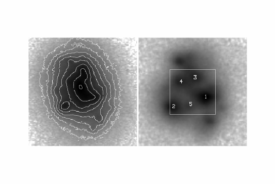
Figure 1: Left panel: $B$-band image of Mrk 1418 with isocontours, spaced 0.5 mag apart, overlaid. Right panel: continuum subtracted H$\alpha$ frame, with the $16\times 16$ arcsec${}^{2}$ PMAS field of view overlaid and the main star-forming knots labeled. North is up, east to the left. Both images are from Gil de Paz et al. (2003), and publicly available in the NED; the PSF is $2\aas@@fstack{\prime\prime}6$ FWHM.

To study the galaxy morphology we use flux maps of the brightest emission lines and the two continuum bands above. The emission line maps trace the interstellar gas, ionized by massive stars, while the continuum maps show the stellar light distribution. For comparison, Figure 1 displays the published $B$ broad-band and H$\alpha$ images of Mrk 1418 (Gil de Paz et al. 2003), with the field of view covered by the PMAS observations overplotted. There is good qualitative agreement between the reconstructed maps (see Figure 2) and the direct images.

Figure 2 displays the emission line flux maps in [O ii] $\lambda 3727$, H$\beta$, [O iii] $\lambda 5007$, H$\alpha$, [N ii] $\lambda 6584$, and [S ii] $\lambda\lambda 6717,\;6731$. The galaxy shows the same morphology in all emission lines: five SF knots are distributed in a roughly circular pattern around the optical center of the galaxy. The emission peak is located in knot 1 in all the lines (see Figure 1), in the western part of the galaxy. This large knot seems to be connected with knot 4, placed $\approx 10\arcsec$ to the northeast, with a bridge-like structure.

In the continuum (see bottom panels in Figure 2), Mrk 1418 shows an inner kidney-shaped feature, with a peak located approximately at the center of the outer isophotes. The position of this central maximum in the continuum frames does not depend on what specific “emission line free” spectral range is used, hence we can safely define this continuum peak as the optical nucleus of the galaxy. Smaller condensations are detected north and southeast of the galaxy nucleus.

The structure of the ionized gas, as traced by the emission lines, looks quite different from the stellar light distribution. At the position of the continuum peak, there is a dearth of gas emission, indicating that the star formation in the central regions has already ceased. The position of the knots detected in emission does not coincide with any continuum peak (knot 2 is close, but not coincident with the continuum blob seen in the southeast corner). Knots 3 and 4 seem to be co-located with a shallow, local blue maximum in the ”blue–red” continuum map, while knots 1 and 2 are slightly displaced from the blue continuum peaks.

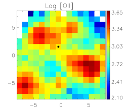
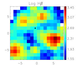
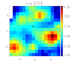
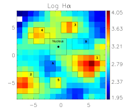
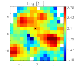
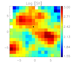
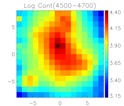
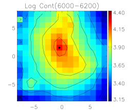
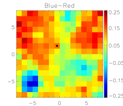
Figure 2: Emission line maps for [O ii] $\lambda$3727, H$\beta$, [O iii] $\lambda 5007$, H$\alpha$, [N ii] $\lambda 6584$ and [S ii] $\lambda\lambda 6717,\;6731$, continuum maps in the intervals 4500–4700 Å (blue) and 6000–6200 Å (red), and the continuum color map. Axis units are arcseconds; north is up, east to the left. Maps are in logarithmic scale (in units of $10^{-18}$ erg s${}^{-1}$ cm${}^{-2}$), except the “blue–red” continuum color map which is in magnitudes (with arbitrary zero point). The black dot marks the nucleus of the galaxy, defined as the peak in the continuum frames. The H$\alpha$ map also shows the outline of the SF knots and of the two ”interknot” regions, A and B (see text for details). The isophotes of the “red” continuum map are spaced 0.2 dex apart.

3.2 Ionization: mechanism and structure

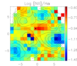
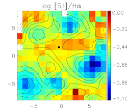
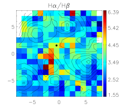
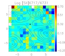
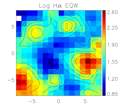
Figure 3: Line ratios maps: [O iii] $\lambda 5007$/ H$\beta$, [N ii] $\lambda 6584$/ H$\alpha$, [S ii] $\lambda\lambda 6717,\;6731$/ H$\alpha$, H$\alpha$/ H$\beta$  and [S ii] $\lambda 6717$/[S ii] $\lambda 6731$. The last panel shows the H$\alpha$ equivalent width map. H$\alpha$ contours (spaced 0.2 dex apart) have been overlaid in all the maps. Axis units are arcseconds; north is up, east to the left. All maps are in logarithmic scale, except H$\alpha$/H$\beta$. The black dot marks the nucleus of the galaxy.

To obtain information about the ionization structure of the ionized nebulae and the nature of the ionization sources acting in Mrk 1418, we built emission line ratio maps in [O iii] $\lambda 5007$/H$\beta$, [N ii] $\lambda 6584$/H$\alpha$  and [S ii] $\lambda\lambda 6717,\;6731$/H$\alpha$. Although [O i] $\lambda 6300$ is detectable in many spaxels, it unfortunately falls very close to the sky line [O i] $\lambda 6300$, which prevents us from obtaining precise measurement of its flux and, hence, of the [O i] $\lambda 6300$/H$\alpha$ ratio.

Using the information derived from the above mentioned line ratios it is possible to distinguish among the different ionization mechanisms acting in a gaseous nebula, namely, photoionization by radiation from OB stars, shock-wave heating and photoionization by a power law continuum source (Baldwin et al. 1981; Veilleux & Osterbrock 1987). The [O iii] $\lambda 5007$/H$\beta$ emission line ratio is an excitation parameter indicator and provides information about the available fraction of hard ionizing photons of the ionizing star cluster embedded in the nebula; therefore a large [O iii] $\lambda 5007$/H$\beta$ ratio indicates a highly ionized region. [N ii] $\lambda 6584$ and [S ii] $\lambda\lambda 6717,\;6731$ are low ionization lines, usually weak in H ii regions: large [N ii] $\lambda 6584$/H$\alpha$ and [S ii] $\lambda\lambda 6717,\;6731$/H$\alpha$ ratios usually indicate the presence of ionizing mechanisms different from photoionization, e.g. shock waves and/or AGNs (e.g. Shull & McKee 1979).

Figure 3 displays the maps of [O iii] $\lambda 5007$/H$\beta$, [N ii] $\lambda 6584$/H$\alpha$ and [S ii] $\lambda\lambda 6717,\;6731$/H$\alpha$. In order to allow a quick comparison with the position of the ionization sources, H$\alpha$ contours have been overlaid. These three maps show basically the same structure. As expected in regions photoionized by stars, they trace the star-formation activity, and the peaks in [O iii] $\lambda 5007$/H$\beta$ coincide with the minima in [N ii] $\lambda 6584$/H$\alpha$ and [S ii] $\lambda\lambda 6717,\;6731$/H$\alpha$. Only knot 4 displays a different behavior: it is a moderate minimum in [N ii] $\lambda 6584$/H$\alpha$ and [S ii] $\lambda\lambda 6717,\;6731$/H$\alpha$  and also shows low values in [O iii] $\lambda 5007$/H$\beta$. The [O iii] $\lambda 5007$/H$\beta$ map also displays a peak at about $(-2\arcsec,-2\arcsec)$, the same position as the peak in the extinction map, in an area that does not coincide with any emission knot.

3.3 Extinction

The extinction map was built from the H$\alpha$/H$\beta$ ratio. No reliable fits could be obtained, for the individual spaxels, for H$\delta$ and H$\gamma$, as they are much weaker and are also strongly affected by underlying stellar absorption.

The H$\alpha$/H$\beta$ ratio map is shown in Figure 3. Mrk 1418 shows an inhomogeneous extinction pattern, which peaks in the central, inter-knot regions, displaced from the continuum maximum ($\approx 3\arcsec$ to the southeast). There, H$\alpha$/H$\beta$ varies between 4 and 5.5, suggesting strong extinction by dust with a reddening $E(B-V)$ of up to 0.62 mag, while in the surrounding SF knots the H$\alpha$/H$\beta$ ratio is $\leq 3$, that is $E(B-V)\leq 0.04$ mag. Indeed, an extinction patch or lane located between the emission line knots has been already observed in several BCDs (e.g. García-Lorenzo et al. 2008; Vanzi et al. 2008; Kehrig et al. 2008), and could be related to the sweeping out of the ISM by stellar winds and SNs. In the continuum ”blue–red” color map, the position of the extinction peak is redder than the knots, but no dust lane or patch is clearly seen; changes in stellar populations as well as the specific geometry of the dust distribution may account for this seeming incongruity.

This result stresses the importance of performing a bidimensional correction of the interstellar extinction: just assuming a single, spatially constant value for the extinction can lead to large errors in the derivation of fluxes and magnitudes in the different regions of the galaxy. As an example, if we used the extinction value for knot 1, $E(B-V)\sim 0.07$, to correct the observed colors in the nuclear region (where the extinction is $E(B-V)\sim 0.40$) we would obtain a color $B-V$ about 0.3 mag redder than its actual value.

3.4 Electron density distribution

We also produced the map of the ratio [S ii] $\lambda 6717$/[S ii] $\lambda 6731$, an electron number density sensitive diagnostic for the range 100–10.000 cm${}^{-3}$ (Figure 3). We find that the density is almost constant, with values close to the low density limit in almost the whole field of view. Only in a few fibers in the central, inter-knot region (the same one where the peaks of the [O iii] $\lambda 5007$/H$\beta$ ratio and of the extinction are located) the density is higher.

3.5 Integrated spectroscopy of selected galaxy regions

As the next step in our spectroscopic analysis, we used the derived flux and continuum maps to isolate the regions of interest in the central parts of the galaxy. They include the five brightest SF knots detected in the narrow-band maps and the nucleus, defined as the continuum peak (see Figure 2).

We identified the fibers corresponding to each region, and summed their spectra together to create the final spectrum. The regions were defined as those spaxels with an H$\alpha$ flux larger than 3.2 (in logarithm), a threshold chosen as the best compromise between enclosing a sufficient number of spaxels for each knot, and avoiding that the knots overlap or abut each other. A few spaxels above this threshold but whose inclusion would have stretched the shape of a knot were excluded, while knot 5 was augmented by two additional spaxels below the threshold.

We also defined two interknot regions: A, where the H$\alpha$ flux has a local minimum, and B, where the [S ii] $\lambda\lambda 6717,\;6731$/H$\alpha$ ratio is highest (see Figure 2).

In this way we produced higher signal-to-noise spectra (in comparison to the spectra of the individual fibers), better suited to derive physical parameters and chemical abundances. The area of these regions ranges between $\sim 0.02$ and 0.10 kpc${}^{2}$. We also computed the total spectrum of Mrk 1418 by summing all the 256 spaxel spectra (that is, over an area of 1.3 kpc${}^{2}$).

Figure 4: Spectra of the 5 knots, of the nucleus, and the total spectrum obtained by summing all the fibers. Spectra are shown in logarithmic scale and are offset for clarity. Small tickmarks are spaced 0.2 dex apart.

Fig. 4 displays the spectra for the six selected regions and the whole mapped field of view. The spectra of the five SF regions show similar characteristics: all of them are dominated by strong emission features, superimposed on a blue continuum. Strong [O ii] $\lambda 3727$, H$\beta$, [O iii] $\lambda 5007$, H$\alpha$, [N ii] $\lambda 6584$ and [S ii] $\lambda\lambda 6717,\;6731$, are visible in emission. Absorption wings are detected in H$\delta$, H$\gamma$ and H$\beta$, for knots 3, 4, and 5. Although [O i] $\lambda 6300$ is detected in the spectra of all the five knots, no reliable flux measurements could be obtained, as the profile of this line is contaminated by the residuals from the subtraction of the [O i] $\lambda 6300$ sky-line. The spectrum of the nucleus shows strong absorption features, indicating an important contribution of older stars; H$\delta$, H$\gamma$ and higher order Balmer lines (H11, H10, H9, H8, H7) are visible only in absorption.

3.5.1 Reddening corrected line fluxes

Fluxes and equivalent widths of the emission lines were measured by fitting the line profile with a Gaussian. Reddening-corrected intensity ratios and equivalent widths for the different spatial regions are listed in Table 2. The correction from underlying stellar absorption was done in two different ways, as explained below.

In knots 4 and 5, and in the nuclear and the integrated spectra, the H$\beta$ Balmer line shows clear absorption wings, and we fitted simultaneously an absorption and an emission component.

In the remaining cases, we proceeded as follows. We first adopted an initial estimate for the absorption equivalent width, EW${}_{\mathrm{abs}}$, corrected the measured fluxes, and computed the extinction coefficient $C(\mbox{H$\beta$})$ through a least-square fit to the Balmer decrement given by the equation:

$$\frac{F(\lambda)}{F(\mbox{H$\beta$})}=\frac{I(\lambda)}{I(\mbox{H$\beta$})}\times 10^{C({\rm H}\beta)\times f(\lambda)}$$ (1)

where $\frac{F(\lambda)}{F({\rm H}\beta)}$ is the line flux corrected for absorption and normalized to H$\beta$; $\frac{I(\lambda)}{I({\rm H}\beta)}$ is the theoretical value for case B recombination, from Brocklehurst (1971), and $f(\lambda)$ is the reddening curve normalized to H$\beta$ which we took from Whitford (1958).

We then varied the value of EW${}_{\mathrm{abs}}$, until we find the one that provides the best match (e.g. the minimum scatter in the above relation) between the corrected and the theoretical line ratios. This is done separately for each knot.

We note that this correction accounts for the fraction of emission line flux that is masked by the underlying absorption, and not necessarily represents the actual absorption equivalent width. To illustrate this point, let us consider two (extreme) examples: (1) the width of the emission line and that of the absorption line are very similar; in this case the absorption component is completely hidden underneath the stronger emission component, and the measured emission flux will be the algebraic sum of the fluxes of the two components (the flux of the absorption line being negative); (2) the absorption line is very broad and shallow; in this case, the emission line flux measured by setting the continuum level on both sides of the “base” of the emission line profile will only slightly underestimate the actual flux, and the correction will be much smaller that the actual equivalent width of the absorption component.

We compared our measurements for the integrated and the nuclear spectra with the spatially integrated (within a $30\arcsec\times 50\arcsec$ area) and nuclear ($2\aas@@fstack{\prime\prime}5\times 2\aas@@fstack{\prime\prime}5$) values published by Moustakas & Kennicutt (2006). The results are presented in Fig. 5: keeping into account the different sizes of the apertures used, and a likely small spatial offset in the location of the nuclear aperture, the comparison looks fair.

Figure 5: Comparison between the integrated and nuclear fluxes and equivalent widths from this paper (TP), and the values published by Moustakas & Kennicutt (2006) (M&K), which used apertures of $30\arcsec\times 50\arcsec$ and $2\aas@@fstack{\prime\prime}5\times 2\aas@@fstack{\prime\prime}5$ respectively. For this comparison, our measurements have only been corrected for galactic extinction and, for the Balmer lines, for underlying absorption (see text for details). Filled circles represent the integrated spectra, open circles correspond to the nuclear spectra. The line at $\simeq 4350$ Å is H$\gamma$.

3.5.2 Line ratios, physical parameters and chemical abundances

Table 3 lists the most relevant line ratios, physical parameters and chemical abundances for the selected regions in Mrk 1418. In order to calculate the errors associated with the physical properties and chemical abundances, we propagated the emission-line intensity errors listed in Table 2.

The physical conditions (electron density and temperature) and ionic element abundances were derived from the reddening-corrected emission line fluxes following the 5-level atom fivel program in the IRAF nebular package (De Robertis et al. 1987; Shaw & Dufour 1995).

Electron densities were calculated from the ratio of [S ii] $\lambda$6717/$\lambda$6731 emission lines. The electron temperature of [O iii] ($T_{\mathrm{e}}$[O iii]), representative of the high-excitation zone of the ionized gas, was derived from the [O iii] $\lambda$4363/($\lambda$4959+$\lambda$5007) ratio for knots 1 and 2, and for the summed spectrum. In order to calculate $T_{\mathrm{e}}$[O ii] we used the relation between [O ii] and [O iii] electron temperatures from Pilyugin et al. (2006). We assumed the approximation $T_{\mathrm{e}}$[S ii] $\approx T_{\mathrm{e}}$[N ii] $\approx T_{\mathrm{e}}$[O ii] for the calculation of S${}^{+}$ and N${}^{+}$ abundances, since no auroral line could be measured in the low excitation zone. We adopted $T_{\mathrm{e}}$[O iii] for the calculation of O${}^{2+}$. As the nebular He ii $\lambda 4686$ Å  line was not detected in any of the knot spectra, we can assume that the contribution from highly ionized species like O${}^{3+}$ is negligible. Therefore, the total oxygen and nitrogen abundances were obtained as: $\mathrm{O/H}=(\mathrm{O}^{+}+\mathrm{O}^{2+})/\mathrm{H}^{+}$ and $\mathrm{N/O}=\mathrm{N}^{+}/\mathrm{O}^{+}$.

To obtain oxygen abundances in those knots in which [O iii] could not be measured (knots 3, 4, 5, and the nucleus), we applied the commonly used strong-line method from Pettini & Pagel (2004). These authors revised the $N2$ ($\equiv$ log[N ii] $\lambda 6584$/H$\alpha$) and $O3N2$ ($\equiv$ log{([O iii]$\lambda 5007$/H$\beta$)/([N ii]$\lambda 6584$/H$\alpha$)}) indices, using 137 extragalactic H ii regions. The uncertainties in the derived metallicities from these two indices are $\sim 0.38$ and 0.25 dex respectively.

For knots 1 and 2, the estimated oxygen abundances from empirical parameters are consistent, within the uncertainties, with those derived using the electron temperature.

The position of the five SF regions in the diagnostic diagram: [O iii] $\lambda 5007$/H$\beta$ vs [N ii] $\lambda 6584$/H$\alpha$ and [S ii] $\lambda\lambda 6717,\;6731$/H$\alpha$, is shown in Fig. 6. The empirical boundaries between the different zones (from Veilleux & Osterbrock 1987), as well as the theoretical boundaries proposed by Kewley et al. (2001), are also plotted. In both diagrams, all the SF knots fall within the area occupied by H ii regions.

Figure 6: Optical emission-line diagnostic diagram for the different SF knots and the two interknot regions (A and B). The curves separate Seyfert galaxies, LINERS and H ii regions-like objects; solid lines are the empirical boundaries from Veilleux & Osterbrock (1987), while dotted lines are the theoretical boundaries from Kewley et al. (2001).

3.6 Kinematics of the ionized gas

We obtained the velocity field by fitting a single Gaussian to the strong H$\alpha$ and [O iii] $\lambda 5007$ emission lines.

Results are displayed in Fig. 7. No regular pattern is visible in these maps, whereas some rotation is expected in the innermost $10\arcsec$, where the velocity changes from 760 to 800 km/s in the radio data by van Zee et al. (2001) (see their Fig. 12). Given the spectral resolution of our data, $\sim 300$ km s${}^{-1}$ at H$\alpha$ and $\sim 400$ km s${}^{-1}$ at O iii, velocity structures can not be reliably measured. An analysis of the kinematics of Mrk 1418 in the optical has to await data taken with higher spectral resolution.

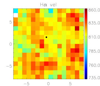
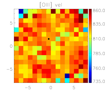
Figure 7: Velocity field of the ionized gas in the central region of the galaxy for the [O iii] $\lambda 5007$ and the H$\alpha$ lines. Axis units are arcseconds; north is up, east to the left.

4 Discussion

Results based on PMAS IFS observations of the BCD Mrk 1418 are presented. The mapped area covers the central starburst region of the galaxy ($16\times 16$ arcsec${}^{2}$, equal to $1.14\times 1.14$ kpc${}^{2}$; see Fig. 1).

The emission line and continuum maps reveal quite an intriguing structure. Both gas and stars display an irregular morphology; interestingly, none of the peaks in the ionized gas maps coincides with a maximum in the continuum. Small spatial offsets between continuum and emission line peaks are common in compact starburst galaxies, as reported for instance by Hunter & Thronson (1995), Maiz-Apellaniz et al. (1998) and Lagos et al. (2007), and are likely related to the release of kinetic energy by massive stars and supernova explosions.

In the emission lines, at least five major knots are resolved; the two biggest ones, knot 1 and knot 2, have approximate diameters of 400 pc and 300 pc respectively. These sizes are comparable to those typical of giant H ii regions in M 33 (e.g., NGC 604;Sandage & Tammann 1974) and in the LMC (e.g., 30 Dor; Walborn 1991).

In the continuum maps a bright nucleus is located in the central part of the field of view, in a place with reduced H$\alpha$ emission (see Figure 2). In the continuum the galaxy shows a distorted, kidney-shaped morphology, with boxy isocontours, which can be seen with better clarity in the $B$-band image in Fig. 1 and in the red continuum image in Fig. 2 (see contours). Such boxy morphology, though usually interpreted as a sign of interactions or mergers (Doublier et al. 1997, 1999), can just be the result of the superposition of the starburst on an older, more regular stellar component.

The current SF activity is taking place in the five major line-emitting knots (Fig. 2), while the lack of significant gas emission in the nuclear region suggests the presence of a dominating intermediate age population. The underlying host galaxy detected in broad-band images (Doublier et al. 1997; Gil de Paz et al. 2003) shows colors ($B-R\sim 1.5-1.7$; Doublier et al. 1997; Gil de Paz & Madore 2005) indicative of a population several Gyrs old.

The ages of the selected regions have been estimated by comparing their H$\alpha$ and H$\beta$ equivalent with the predictions from Starburst 99 (Leitherer et al. 1999) evolutionary synthesis models. We chose those models with $Z=0.4\leavevmode\nobreak\ Z\sun$, the closest value to the metallicity derived from the emission-line fluxes — a reasonable approximation to the metallicity of a young population — and a Salpeter initial mass function (IMF) between 1 and 100 $M_{\sun}$. We found that we can reproduce the measured H$\alpha$ and H$\beta$ equivalent widths for the five SF knots with an instantaneous burst of star formation and ages ranging between 5 and 7 Myr: knots 1 and 2 seem to be the youngest, with equivalent widths consistent with ages between 5 and 6 Myr, while for knots 3, 4 and 5, we found values slightly larger, from 6 to 7 Myr. The equivalent widths in the nucleus are consistent with ages of about 10 Myr.

We should keep in mind that these values are indeed upper limits to the ages of the knots. In fact, as the continuum flux increases due to the contribution from the older stars, the measured equivalent widths decrease and this in turn results into larger derived ages for the knots. As shown in previous works (Cairós et al. 2002, 2007), this effect is not negligible in BCDs, though difficult to quantify: it rests on the model adopted to describe the underlying component and can strongly vary with the position of the knots across the galaxy. For instance, the corrections found for the different knots in the galaxy Mrk 35 range from 10% to 90% (Cairós et al. 2007). By assuming a contribution of the host galaxy of 50% to the continuum in the brightest knots in Mrk 1418, the computed age will be about 1 Myr less.

The Interstellar Medium (ISM) around the SF knots is excited by the ionizing photons coming from the central stars/clusters, with no clear evidence for other excitation mechanisms. In the “interknot” area B a moderate [O iii] $\lambda 5007$/H$\beta$ ratio together with a large [S ii] $\lambda\lambda 6717,\;6731\leavevmode\nobreak\$/H$\alpha$ ratio (see Fig. 6) suggest that some mechanisms other than photoionization contribute to the gas excitation (most probably shocks; e.g. Shull & McKee 1979; Schwartz et al. 1993).

On the other hand, nebular He ii $\lambda 4686$ Å emission has been detected (in one just spaxel) in a location southwest of the galactic center (near knot 2). This line offers a powerful diagnostic of the ionizing fluxes and stellar population in starburst regions but, unfortunately, here its $S/N$ is too poor for a reliable measurements of its FWHM and flux.

The interstellar extinction has an overall irregular distribution, with a ridge that crosses the galaxy in a north-south direction between knots 2 and 5, consistent with material swept out by stellar winds and SNe. Its position and shape are in broad agreement with a dust-lane visible in the SDSS frames. This finding is in line with recent publications (Hunt et al. 2001; Cairós et al. 2003; Vanzi & Sauvage 2004; Cairós et al. 2007) that questioned the previous belief that BCDs have little or no dust. Leroy et al. (2005) report Mrk 1418 as a nondetection in their CO survey.

In agreement with several other works on BCDs (e.g. Izotov et al. 1997; Vílchez & Iglesias-Páramo 1998; Papaderos et al. 2006; Kehrig et al. 2008), we did not find any significant chemical abundance variation among the different knots in the galaxy, which points to a common chemical evolution scenario in all of them. Also, the nitrogen-to-oxygen abundance ratio values found are consistent with those obtained for BCDs and H ii galaxies (Vílchez & Iglesias-Páramo 2003; Pérez-Montero & Díaz 2005).

We found for the total spectrum a lower value of direct oxygen abundance and a higher electron temperature than for knots 1 and 2 (see Table 3). While this finding may reflect a genuine difference between the oxygen abundance in the total spectrum (kpc-sized aperture) and in the individual H ii regions (with sizes of the order of 100 pc), it may also be due to the relatively large measurement uncertainties for the weak [O iii] $\lambda$4363 emission line.

The origin of the starburst episodes in SF dwarf galaxies is far from being well understood. One of the current scenarios is the stochastic self-propagating star formation (SSPSF) model proposed by Gerola et al. (1980), in which the starburst episode in dwarfs is explained as statistical fluctuations in the SFR. In Mrk 1418 both the ages of the starburst and the morphology speak against this scenario; the different SF knots have ages too similar to be causally related: with the typical distances among knots (400–800 pc), the star formation will need times of the order of 40–80 Myr to propagate through shock traveling at a typical speed of $\sim 10$ km s${}^{-1}$.

An alternative scenario, which is gaining popularity, is interactions and mergers. Recent searches have shown that a substantial fraction of SF dwarfs possess low-mass companion galaxies, most of them gas-rich but faint in the optical (Taylor et al. 1993, 1995, 1996; Noeske et al. 2001; Pustilnik et al. 2001), while studies focused on individual objects have shown that interactions indeed play a substantial role in the evolution of these systems (Johnson et al. 2004; Östlin et al. 2004; Bravo-Alfaro et al. 2004, 2006; Cumming et al. 2008 – but see Vaduvescu et al. 2007).

These observational results have been recently backed up from the theoretical point of view. The numerical simulations presented in Bekki (2008) can satisfactory explain the physical properties of BCDs (e.g. blue compact core, redder low surface brightness component, presence of compact young stellar clusters, low metallicity and extended HI gas disk) as the result of mergings between dwarfs with larger fraction of gas and extended gas disks.

In Mrk 1418, the asymmetric spatial distribution of the SF knots, their different sizes, the bridge-like structure connecting knot 1 and knot 4, and the filamentary structures visible in the NED H$\alpha$ image, as well as the boxy, kidney-shape morphology of the continuum, are all suggestive of a system that has recently experienced some interaction events. Kinematic results from H i maps (van Zee et al. 2001) also agree with a merger/interaction scenario: the extended gaseous distribution show kinematical peculiarities, reminiscent of tidal tails. The H i velocity field displays a complex behavior in the inner regions, but an overall clear rotation pattern.

The low velocity resolution of our PMAS data hampers the derivations of a reliable velocity distribution. Deeper, higher spectral resolution IFU observations, aimed at measuring the gas velocity dispersion as well as the stellar kinematics, are essential to put tighter constraints on the galaxy dynamics.

5 Conclusions

The central $16\arcsec\times 16\arcsec$ region of the BCD galaxy Mrk 1418 has been mapped by using the PMAS spectrograph. Integral Field Spectroscopy allowed us to simultaneously study the morphology, ionization mechanism, extinction, chemical abundances and ionized gas kinematics of the galaxy. From our analysis we highlight the following results:

1. Mrk 1418 displays very different morphologies in the continuum and in the emission lines. While in the continuum the central region has a distorted, kidney-like shape and boxy isocontours, with the peak located approximately at the center of the outer isophotes, the emission line maps exhibit five SF regions irregularly distributed around the optical center.

2. The excitation ratios [O iii]/H$\beta$ and [N ii]/H$\alpha$ are typical of H ii regions in the whole mapped area, while in the interknots zones (region B) the [S ii]/H$\alpha$ ratios have values $\geq 0.4$, possibly indicating the presence of shocks.

3. The galaxy displays an inhomogeneous dust distribution, with a peak value $\mbox{H$\alpha$}/\mbox{H$\beta$}=5.5$ in the region between knot 2 and knot 5, about $3\arcsec$ southeast of the continuum peak; this dust patch has an area of about $8\squareforqed\arcsec$.

4. For each SF knot we derived line fluxes, interstellar extinction, the most relevant line ratios and metal abundances. We find that: i) all the knots show H ii-like ionization (e.g. star formation); ii) the density does not vary significantly from knot to knot, and has values typical of giant extragalactic objects (McCall et al. 1985); iii) all knots have similar metal abundance, with no abundance variations on scales of hundreds of parsec.

This pilot paper shows that IFS is an essential tool to study BCD galaxies, as, in just one shot, it allows us to map the gas and stars morphology, determine the physical parameters and derive chemical abundances.

Therefore, IFU studies of large BCD samples will enable us to gain insights into the main issues concerning this class of galaxies, namely, to disentangle and characterize their stellar populations, to elaborate their SF histories and to investigate the mechanisms that trigger their star-formation activity.

Table 2: Reddening corrected line ratios, normalized to H$\beta$${}^{(*)}$, for the knots identified in Mrk 1418.

$\lambda$	Ion	knot 1		knot 2		knot 3		knot 4		knot 5		Nucleus		Integrated
		F${}_{\lambda}$	-W${}_{\lambda}$	F${}_{\lambda}$	-W${}_{\lambda}$	F${}_{\lambda}$	-W${}_{\lambda}$	F${}_{\lambda}$	-W${}_{\lambda}$	F${}_{\lambda}$	-W${}_{\lambda}$	F${}_{\lambda}$	-W${}_{\lambda}$	F${}_{\lambda}$	-W${}_{\lambda}$
3727	[O ii]	$3.19\pm 0.27$	$82.14\pm 0.93$	$3.43\pm 0.30$	$62.70\pm 1.03$	$3.10\pm 0.31$	$52.25\pm 1.81$	$6.00\pm 0.56$	$117.2\pm 3.53$	$5.24\pm 0.57$	$65.37\pm 3.65$	$10.45\pm 1.38$	$23.53\pm 0.78$	$5.44\pm 0.43$	$43.28\pm 0.25$
3869	[Ne iii]	$0.51\pm 0.04$	$11.72\pm 0.44$	$0.39\pm 0.03$	$7.94\pm 0.44$	$0.56\pm 0.07$	$7.34\pm 0.77$	$0.43\pm 0.12$	$6.27\pm 1.40$	$0.83\pm 0.20$	$7.68\pm 1.62$	—	—	$1.00\pm 0.07$	$7.70\pm 0.12$
3968	[Ne iii]	$0.19\pm 0.02$	$4.66\pm 0.30$	$0.18\pm 0.02$	$3.74\pm 0.36$	—	—	—	—	—	—	—		—	—
4101	H$\delta$	$0.28\pm 0.02$	$6.82\pm 0.22$	$0.30\pm 0.02$	$7.31\pm 0.32$	$0.37\pm 0.07$	$5.31\pm 0.46$	$0.26\pm 0.08$	$3.93\pm 0.71$	—	—	—	—	—	—
4340	H$\gamma$	$0.46\pm 0.02$	$12.95\pm 0.23$	$0.46\pm 0.03$	$13.37\pm 0.33$	$0.46\pm 0.04$	$7.21\pm 0.36$	$0.47\pm 0.05$	$8.28\pm 0.60$	$0.47\pm 0.07$	$6.91\pm 0.63$	—	—	$0.47\pm 0.02$	$4.29\pm 0.05$
4363	[O iii]	$0.05\pm 0.01$	$2.00\pm 0.23$	$0.05\pm 0.01$	$2.29\pm 0.37$	—	—	—	—	—	—	—	—	$0.10\pm 0.04$	$1.02\pm 0.06$
4861	H$\beta$	$1.00$	$31.27\pm 0.25$	$1.00$	$32.96\pm 0.34$	$1.00$	$17.42\pm 0.39$	$1.00$	$18.30\pm 0.90$	$1.00$	$12.73\pm 0.68$	$1.00$	$3.03\pm 0.24$	$1.00$	$10.14\pm 0.06$
4959	[O iii]	$1.24\pm 0.04$	$38.81\pm 0.29$	$1.16\pm 0.03$	$41.07\pm 0.44$	$1.12\pm 0.05$	$19.89\pm 0.41$	$0.61\pm 0.04$	$11.54\pm 0.48$	$1.14\pm 0.08$	$15.78\pm 0.66$	$0.83\pm 0.09$	$2.61\pm 0.18$	$1.06\pm 0.03$	$11.01\pm 0.06$
5007	[O iii]	$3.62\pm 0.10$	$113.9\pm 0.46$	$3.45\pm 0.10$	$122.70\pm 0.51$	$3.19\pm 0.12$	$55.06\pm 0.49$	$1.78\pm 0.09$	$34.54\pm 0.54$	$3.29\pm 0.18$	$46.81\pm 0.90$	$2.34\pm 0.20$	$7.61\pm 0.20$	$3.16\pm 0.09$	$33.48\pm 0.09$
5876	He i	—	—	$0.07\pm 0.01$	$3.11\pm 0.21$	$0.11\pm 0.01$	$2.48\pm 0.26$	$0.07\pm 0.01$	$1.88\pm 0.35$	$0.08\pm 0.02$	$1.60\pm 0.49$	—	—	$0.05\pm 0.01$	$0.75\pm 0.03$
6548	[N ii]	$0.08\pm 0.01$	$3.69\pm 0.19$	$0.15\pm 0.01$	$8.15\pm 0.44$	$0.10\pm 0.02$	$2.65\pm 0.34$	$0.13\pm 0.02$	$3.77\pm 0.47$	$0.10\pm 0.03$	$2.37\pm 0.62$	$0.12\pm 0.03$	$0.80\pm 0.21$	$0.11\pm 0.01$	$1.95\pm 0.05$
6563	H$\alpha$	$2.87\pm 0.10$	$137.6\pm 0.39$	$2.88\pm 0.14$	$154.1\pm 1.35$	$2.90\pm 0.20$	$73.72\pm 0.79$	$2.87\pm 0.15$	$84.12\pm 1.41$	$2.87\pm 0.16$	$69.03\pm 1.48$	$2.86\pm 0.34$	$19.63\pm 0.27$	$2.86\pm 0.07$	$49.87\pm 0.10$
6584	[N ii]	$0.26\pm 0.01$	$12.50\pm 0.23$	$0.29\pm 0.02$	$15.22\pm 0.43$	$0.22\pm 0.02$	$5.68\pm 0.40$	$0.31\pm 0.03$	$9.14\pm 0.61$	$0.19\pm 0.03$	$4.56\pm 0.61$	$0.33\pm 0.05$	$2.25\pm 0.20$	$0.27\pm 0.01$	$4.63\pm 0.06$
6717	[S ii]	$0.26\pm 0.01$	$12.50\pm 0.28$	$0.31\pm 0.02$	$17.05\pm 0.44$	$0.31\pm 0.03$	$8.21\pm 0.44$	$0.42\pm 0.03$	$12.93\pm 0.60$	$0.29\pm 0.03$	$7.30\pm 0.66$	$0.58\pm 0.08$	$4.21\pm 0.23$	$0.40\pm 0.01$	$8.49\pm 0.05$
6731	[S ii]	$0.21\pm 0.01$	$10.22\pm 0.25$	$0.23\pm 0.02$	$12.69\pm 0.43$	$0.20\pm 0.02$	$5.43\pm 0.41$	$0.32\pm 0.02$	$9.87\pm 0.57$	$0.20\pm 0.03$	$5.17\pm 0.68$	$0.42\pm 0.06$	$3.02\pm 0.21$	$0.30\pm 0.01$	$5.52\pm 0.07$
		$F(\mbox{H$\beta$})=324.6\pm 22.7$		$F(\mbox{H$\beta$})=166.3\pm 15.2$		$F(\mbox{H$\beta$})=67.4\pm 11.3$		$F(\mbox{H$\beta$})=84.6\pm 6.0$		$F(\mbox{H$\beta$})=42.4\pm 3.9$		$F(\mbox{H$\beta$})=106.3\pm 30.4$		$F(\mbox{H$\beta$})=1871.9\pm 62.6$
		$C(\mbox{H$\beta$})=0.111\pm 0.032$		$C(\mbox{H$\beta$})=0.073\pm 0.035$		$C(\mbox{H$\beta$})=0.123\pm 0.064$		$C(\mbox{H$\beta$})=0.267\pm 0.025$		$C(\mbox{H$\beta$})=0.361\pm 0.030$		$C(\mbox{H$\beta$})=0.625\pm 0.105$		$C(\mbox{H$\beta$})=0.316\pm 0.011$
		$W_{\mathrm{abs}}=3.2\AA$		$W_{\mathrm{abs}}=2.9\AA$		$W_{\mathrm{abs}}=2.9\AA$		$W_{\mathrm{abs}}=1.7\AA$		$W_{\mathrm{abs}}=1.4\AA$		$W_{\mathrm{abs}}=3.0\AA$		$W_{\mathrm{abs}}=2.1\AA$

(*) Notes. – Reddening-corrected line fluxes, normalized to $F(\mbox{H$\beta$})=1$. Equivalent widths of Balmer lines are corrected for underlying stellar absorption. The reddening coefficients, $C(\mbox{H$\beta$})$, the value of the absorption correction, EW${}_{\mathrm{abs}}$, and the reddening-corrected H$\beta$ flux, $F(\mbox{H$\beta$})(\times 10^{-16}$ ergs cm${}^{-2}$ s${}^{-1}$) are listed for each region. In the nuclear region, only H$\beta$ and H$\beta$ could be measured, so we were unable to compute EW${}_{\mathrm{abs}}$ and $C(\mbox{H$\beta$})$ simultaneously; to determine the latter we assumed EW${}_{\mathrm{abs}}=3.0$. The quoted uncertainties include measurements, flux-calibration and reddening coefficient errors.

Table 3: Physical parameters and abundances

Parameter	knot 1	knot 2	knot 3	knot 4	knot 5	Nucleus	Integrated
$\log\left(\frac{[\mbox{{O {iii}}}]\;\lambda 5007}{\mbox{H$\beta$}}\right)$	$0.56\pm 0.02$	$0.54\pm 0.02$	$0.50\pm 0.03$	$0.25\pm 0.03$	$0.52\pm 0.04$	$0.37\pm 0.05$	$0.50\pm 0.02$
$\log\left(\frac{[\mbox{{N {ii}}}]\;\lambda 6584}{\mbox{H$\alpha$}}\right)$	$-1.04\pm 0.02$	$-1.00\pm 0.02$	$-1.12\pm 0.05$	$-0.97\pm 0.05$	$-1.18\pm 0.09$	$-0.94\pm 0.08$	$-1.03\pm 0.02$
$\log\left(\frac{[\mbox{{S {ii}}}]\;\lambda\lambda 6717,\;6731}{\mbox{H$\alpha$}}\right)$	$-0.79\pm 0.02$	$-0.73\pm 0.02$	$-0.75\pm 0.03$	$-0.59\pm 0.04$	$-0.77\pm 0.07$	$-0.46\pm 0.06$	$-0.61\pm 0.02$
$N_{\mathrm{e}}$([S ii]) (cm${}^{-3}$)	190	$\leq 100$	$\leq 100$	108	$\leq 100$	$\leq 100$	$\leq 100$
$T_{\mathrm{e}}$([O ii]) (10${}^{4}$ K)	$1.18\pm 0.07$	$1.22\pm 0.07$	—	—	—	—	$1.67\pm 0.30$
$T_{\mathrm{e}}$([O iii]) ($10^{4}$ K)	$1.27\pm 0.10$	$1.33\pm 0.10$	—	—	—	—	$1.96\pm 0.42$
$12+\log(O/H)$ – ($T_{e}$)	$8.09\pm 0.06$	$8.03\pm 0.06$	—	—	—	—	$7.71\pm 0.13$
$12+\log(\mathrm{O/H})$ – ($N2$)	8.26	8.28	8.23	8.30	8.20	8.31	8.27
$12+\log(\mathrm{O/H})$ – ($O3N2$)	8.22	8.24	8.21	8.34	8.19	8.31	8.24
$12+\log(\mathrm{S}^{+}/\mathrm{H}^{+})$	$5.87\pm 0.05$	$5.90\pm 0.05$	—	—	—	—	$5.80\pm 0.10$
$12+\log(\mathrm{N}^{+}/\mathrm{H}^{+})$	$6.52\pm 0.05$	$6.59\pm 0.05$	—	—	—	—	$6.26\pm 0.11$
$\log(\mathrm{N/O})$	$-1.29\pm 0.10$	$-1.18\pm 0.10$	—	—	—	—	$-1.27\pm 0.21$

Notes: $T_{\mathrm{e}}$ ([O ii]) derived from the relation: $T_{\mathrm{e}}\mathrm{([{O\textsc{ii}}])}=0.72\times T_{\mathrm{e}}\mathrm{([{O\textsc{iii}}])}+0.26$ found by Pilyugin et al. (2006).
$T_{\mathrm{e}}$ ([O iii]): electron temperature measured from [O iii] $\lambda 4363$
$12+\log(\mathrm{O/H})$ – ($T_{\mathrm{e}}$): direct O/H abundance derived from $T_{\mathrm{e}}$[O iii]
$12+\log(\mathrm{O/H})$ – ($N2$): O/H derived from the $N2$ index (Pettini & Pagel 2004); the associated uncertainty is $\pm 0.38$
$12+\log(\mathrm{O/H})$ – ($O3N2$): O/H derived from the $O3N2$ index (Pettini & Pagel 2004); the associated uncertainty is $\pm 0.25$.