The Bimodality of Accretion In T Tauri Stars and Brown Dwarfs

Abstract

We present numerical solutions of the collapse of prestellar cores that lead to the formation and evolution of circumstellar disks. The disk evolution is then followed for up to three million years. A variety of models of different initial masses and rotation rates allows us to study disk accretion around brown dwarfs and low-mass T Tauri stars, with central object mass $M_{*}<0.2\,M_{\odot}$, as well as intermediate and upper-mass T Tauri stars ($0.2\,M_{\odot}<M_{*}<3.0\,M_{\odot}$). Our models include self-gravity and allow for nonaxisymmetric motions. In addition to the self-consistently generated gravitational torques, we introduce an effective turbulent $\alpha$-viscosity with $\alpha=0.01$, which allows us particularly to model accretion in the low-mass regime where disk self-gravity is diminishing. A range of models with observationally-motivated values of the initial ratio of rotational to gravitational energy yields a correlation between mass accretion rate $\dot{M}$ and $M_{*}$ that is relatively steep, as observed. Additionally, our modeling reveals evidence for a bimodality in the $\dot{M}$–$M_{*}$ correlation, with a steeper slope at lower masses and a shallower slope at intermediate and upper masses, as also implied by observations. Furthermore, we show that the neglect of disk self-gravity leads to a much steeper $\dot{M}$–$M_{*}$ relation for intermediate and upper-mass T Tauri stars. This demonstrates that an accurate treatment of global self-gravity is essential to understanding observations of circumstellar disks.

1. Introduction

Using numerical hydrodynamic simulations, we have recently shown that self-gravitating disks of intermediate- and upper mass T Tauri stars (TTSs) settle into a self-regulated state, with low-amplitude density perturbations persisting for at least several Myr (Vorobyov & Basu, 2007). These perturbations are sustained by swing amplification at the disk’s outer edge. The associated gravitational torques can drive mass accretion rates that are of correct magnitude to explain the observed values across the range of intermediate and upper mass TTSs (Vorobyov & Basu, 2008). These results were used to argue that the empirically observed correlation between mass accretion rate $\dot{M}$ and central object mass $M_{*}$, of the approximate form $\dot{M}\propto M_{*}^{2}$ (e.g. Muzerolle et al., 2003, 2005; Natta et al., 2004; Calvet et al., 2004; Mohanty et al., 2005), can be explained purely on the basis of self-regulated accretion by gravitational torques in self-gravitating circumstellar disks. Nonaxisymmetric structure (and therefore nonaxisymmetric modeling) is required to achieve this result.

However, it is important to note that the approximate $\dot{M}\propto M_{*}^{2}$ empirical relation was only noticed after data were obtained for brown dwarfs (BDs) and combined with the TTS data. The larger dynamic range of masses and accretion rates in a combined plot reveals a relatively steep overall gradient in $\dot{M}$ versus $M_{*}$. Furthermore, there is evidence that the correlation is steeper at lower masses, and shallower at higher masses (Vorobyov & Basu, 2008), although this is complicated by the fact that different techniques are usually employed to determine $\dot{M}$ in the two mass regimes (Muzerolle et al., 2003; Mohanty et al., 2005).

In this paper we model both the lower and upper mass end of the $\dot{M}$–$M_{*}$ correlation, using additional models for BD accretion that start from the collapse of very dense and compact low-mass cores. The low-mass disks that form around low-mass objects in our simulations are nearly axisymmetric and sustain negligible gravitational torques. Therefore, we explore here the possibility that additional processes are at play in the low-mass regime. These processes may depend on instabilities in the low-mass disks that generate turbulence that in turn yields an effective local viscosity. Our model is therefore consistent with the idea that gravitational torques are the driving agent of mass and angular momentum transport in intermediate- to high mass disks, while a mechanism like the magnetorotational instability (MRI) may dominate in low-mass disks. Other workers have arrived at this conclusion based on physical and observational constraints (e.g. Hartmann et al., 2006; Kratter et al., 2008). We are also motivated by the apparent bimodal slope of the $\dot{M}$–$M_{*}$ correlation, implying that two different physical processes may be dominating disk evolution in the two different mass regimes. We note that our models are tracing the accretion processes for radii greater than 5 AU, and we are implicitly assuming that the inner disk maintains the same accretion rate (at least in a time-averaged sense) through unspecified processes. Therefore, even the gravitational-torque-dominated disks may require processes such as the MRI to accomplish the corresponding angular momentum transport in the inner disk (see Armitage et al., 2001; Zhu et al., 2009).

We model the effect of turbulent viscosity with the $\alpha$-prescription (Shakura & Sunyaev, 1973), implemented in a nonaxisymmetric disk, as laid out in §2. It is applied to models of all masses. Protostellar disks are formed from the self-consistent collapse of initially slowly-rotating prestellar cores. The evolution of the disks are then followed for up to three million years. As explained in our previous papers (Vorobyov & Basu, 2005, 2006), this is made possible through the use of the thin-disk approximation and our nonuniform grid. Such long-term calculations, including wide parameter surveys, remain out of reach for fully three-dimensional calculations. We use our results to compare the numerically-derived mass accretion rates with those inferred observationally for TTSs and BDs in the late stage of star formation.

2. Model description

2.1. Basic Equations

Our numerical model is similar to that used recently to simulate the secular evolution of viscous and self-gravitating circumstellar disks (Vorobyov & Basu, 2009). Here, we briefly provide the basic concepts and equations. We use the thin-disk approximation to compute the evolution of rotating, gravitationally bound cloud cores. The numerical integration is started in the prestellar phase, which is characterized by a collapsing starless cloud core, and continues into the late accretion phase, which is characterized by a protostar/disk/envelope system. This ensures a self-consistent formation of circumstellar disks in our numerical simulations. Once the disk has formed, it occupies the innermost regions of our numerical grid, while the envelope occupies the rest of the grid. This means that the mass infall rate onto the disk is actually determined by the dynamics of gas in the envelope, rather than being input through an ad hoc source term. The thin-disk approximation is an excellent means to calculate the evolution for many orbital periods and many model parameters. It is well justified as long as the ratio of the disk scale height $Z$ to radius $r$ does not considerably exceed 0.1. As one of us has recently shown (see figure 7 in Vorobyov, 2009), this condition is fulfilled for solar mass stars having disks of several hundred AU in radius. Our model disks rarely exceed this size, and hence we believe that the thin-disk approximation is justified after the disk formation epoch. This approximation is also reasonable for the prestellar phase, since protostellar cores are found to be disk-like (Jones et al., 2001; Jones & Basu, 2002; Goodwin et al., 2002; Tassis, 2007).

The basic equations of mass and momentum transport in the thin-disk approximation are

$$\frac{{\partial\Sigma}}{{\partial t}} = -\nabla_{p}\cdot\left(\Sigma\mbox{\boldmath$v$}_{p}\right),$$ (1)

$$\Sigma\frac{d\mbox{\boldmath$v$}_{p}}{dt} = -\nabla_{p}{\cal P}+\Sigma\,\mbox{\boldmath$g$}_{p}+(\nabla\cdot\mathbf{\Pi})_{p}\,,$$ (2)

where $\Sigma$ is the mass surface density, ${\cal P}=\int^{Z}_{-Z}Pdz$ is the vertically-integrated form of the gas pressure $P$, $Z$ is the radially and azimuthally varying vertical scale height, $\mbox{\boldmath$v$}_{p}=v_{r}\hat{\mbox{\boldmath$r$}}+v_{\phi}\hat{\mbox{\boldmath$\phi$}}$ is the velocity in the disk plane, $\mbox{\boldmath$g$}_{p}=g_{r}\hat{\mbox{\boldmath$r$}}+g_{\phi}\hat{\mbox{\boldmath$\phi$}}$ is the gravitational acceleration in the disk plane, and $\nabla_{p}=\hat{\mbox{\boldmath$r$}}\partial/\partial r+\hat{\mbox{\boldmath$\phi$}}r^{-1}\partial/\partial\phi$ is the gradient along the planar coordinates of the disk. The gravitational acceleration $\mbox{\boldmath$g$}_{p}$ includes both the gravity of a central point object (when formed) and the self-gravity of a circumstellar disk and envelope. The latter component is found by solving the Poisson integral using the convolution theorem (see Vorobyov & Basu, 2006, for more details). The viscous stress tensor is

$$\mathbf{\Pi}=2\Sigma\,\nu\left(\nabla v-{1\over 3}(\nabla\cdot v)\mathbf{e}\right),$$ (3)

where $\nabla v$ is a symmetrized velocity gradient tensor, $\mathbf{e}$ is the unit tensor, and $\nu$ is the kinematic viscosity. Equation (2) describes the motion of a viscous fluid in the most general form. This equation can be reduced to the usual equation for the conservation of angular momentum of a radial annulus in the axisymmetric accretion disk. The components of $(\nabla\cdot\mathbf{\Pi})_{p}$ in polar coordinates ($r,\phi$) can be found in Vorobyov & Basu (2009).

It is well known that standard collisional viscosity (molecular viscosity) is negligible in application to circumstellar disks. An alternative is an effective turbulent viscosity induced by instabilities in the disk. A prime candidate is the MRI, although other mechanisms of nonlinear hydrodynamic turbulence cannot be completely ruled out due to the large Reynolds numbers involved. We make no specific assumptions about the source of turbulence and parameterize the magnitude of turbulent viscosity using the usual $\alpha$-prescription (Shakura & Sunyaev, 1973)

$$\nu=\alpha\,\tilde{c}_{s}\,Z,$$ (4)

where $\tilde{c}^{2}_{s}=\partial{\cal P}/\partial\Sigma$ is the effective sound speed of (generally) non-isothermal gas. The vertical scale height $Z$ is determined in every computational cell and at every time step of integration using an assumption of local hydrostatic equilibrium in the gravitational field of the central star and the disk (see Vorobyov & Basu, 2009). It is thus important to note that our disks are not razor-thin but have a vertical extent and flaring which are consistent with those predicted from detailed vertical structure models of irradiated accretion disks around T Tauri stars by D’Alessio et al. (1999).

In this paper we present results for a large number of simulations with differing values of physical parameters but a fixed value $\alpha=0.01$. This choice is motivated by our recent analysis of the secular evolution of viscous and self-gravitating disks (Vorobyov & Basu, 2009). We found that if circumstellar disks around solar-mass protostars can generate and sustain turbulence then the temporally and spatially averaged $\alpha$ should lie in the range $10^{-3}-10^{-2}$, in order to be a significant process but not completely destroy the self-regulated structure. Therefore, a choice of $\alpha=0.01$ samples models in which the turbulent viscosity has a significant and even dominant role during the late stages of disk accretion (gravitational torques are still dominant in the early stages for all but the lowest mass disks, as discussed in § 4). The possible influence of different values of $\alpha$ on our results is also discussed in Section 4.

Equations (1) and (2) are closed with a barotropic equation that makes a smooth transition from isothermal to adiabatic evolution at $\Sigma=\Sigma_{\rm cr}=36.2$ g cm^-2:

$${\cal P}=c_{s}^{2}\Sigma+c_{s}^{2}\Sigma_{\rm cr}\left(\Sigma\over\Sigma_{\rm cr}\right)^{\gamma},$$ (5)

where $c_{s}=0.188$ km s^-1 is the sound speed in the initial state, and $\gamma=1.4$. Numerical simulations with $\gamma=1.67$ produce disks that are hotter than those with $\gamma=1.4$. However, we have recently demonstrated that a modest increase in disk temperature has an insignificant effect on the mean mass accretion rates (see figure 8 in Vorobyov & Basu, 2009). Colder disks ($T\sim 40$ K at 10 AU) are more gravitationally unstable and are characterized by spiral modes that are of larger amplitude than those of hotter disks ($T\sim 100$ K at 10 AU). For hotter disks, however, the amplitudes of modes also decrease sharply with increasing order, leaving low-order modes ($m\leq 2$) dominant. As a result, the hotter models have less mode-to-mode interaction that can produce some cancellation in the net gravitational torque. Since the low-order modes are more efficient transport agents, the net effect is to produce comparable mass accretion rates in disks that differ in temperature by a factor of two. A similar result of increasing low-order mode dominance for hotter disks has been found by Cai et al. (2008). We further note that $\gamma$ depends on the disk temperature and hence it may vary radially, with the inner disk being characterized by $\gamma=1.4$ but the outer disk having $\gamma=1.67$. This radial variation in $\gamma$ is expected to decrease the radial temperature gradient in the disk (as compared to the purely $\gamma=1.4$ disk) but is not expected to considerably change the mass accretion rates for the reason outlined above.

Table 1Model parameters

Set	$\beta$	$\Omega_{0}$	$r_{0}$	$r_{\rm out}$	$M_{\rm cl}$	$N$
1	$6.2\times 10^{-4}$	$0.28-0.47$	$2070-3450$	$(1.2-2.0)\times 10^{4}$	$1.2-2.0$	5
2	$1.3\times 10^{-3}$	$0.27-1.33$	$1040-5180$	$(0.6-3.0)\times 10^{4}$	$0.6-3.0$	11
3	$2.5\times 10^{-3}$	$0.37-3.40$	$570-5180$	$(0.3-3.0)\times 10^{4}$	$0.3-3.0$	16
4	$3.7\times 10^{-3}$	$0.52-6.80$	$350-4490$	$(0.2-2.6)\times 10^{4}$	$0.2-2.6$	18
5	$5.1\times 10^{-3}$	$0.53-10.0$	$280-5180$	$(0.16-3.0)\times 10^{4}$	$0.16-3.0$	17
6	$8.0\times 10^{-3}$	$0.67-20.0$	$172-5180$	$(0.1-3.0)\times 10^{4}$	$0.1-3.0$	18
7	$1.2\times 10^{-2}$	$0.80-34.0$	$120-5180$	$(0.07-3.0)\times 10^{4}$	$0.07-3.0$	16
8	$1.6\times 10^{-2}$	$2.30-50.0$	$95-2070$	$(0.06-1.2)\times 10^{4}$	$0.05-1.2$	12
9	$2.0\times 10^{-2}$	$1.60-91.0$	$60-3450$	$(0.04-2.0)\times 10^{4}$	$0.03-2.0$	14
10	$3.2\times 10^{-2}$	$2.0-114.0$	$60-3450$	$(0.04-2.0)\times 10^{4}$	$0.03-2.0$	13

2.2. Initial Conditions and Numerical Technique

We start our numerical simulations from starless cloud cores, which have surface densities $\Sigma$ and angular velocities $\Omega$ typical for a collapsing axisymmetric magnetically supercritical core (Basu, 1997):

$$\Sigma={r_{0}\Sigma_{0}\over\sqrt{r^{2}+r_{0}^{2}}}\>,$$ (6)

$$\Omega=2\Omega_{0}\left({r_{0}\over r}\right)^{2}\left[\sqrt{1+\left({r\over r_{0}}\right)^{2}}-1\right],$$ (7)

where $\Omega_{0}$ is the central angular velocity, $r_{0}$ is the radial scale length defined as $r_{0}=kc_{s}^{2}/(G\Sigma_{0})$ and $k=\sqrt{2}/\pi$. These initial profiles are characterized by the important dimensionless free parameter $\eta\equiv\Omega_{0}^{2}r_{0}^{2}/c_{s}^{2}$ and have the property that the asymptotic ($r\gg r_{0}$) ratio of centrifugal to gravitational acceleration has magnitude $\sqrt{2}\,\eta$ (see Basu, 1997). The centrifugal radius of a mass shell that encloses a mass $m$ and is initially located at radius $r$ is estimated to be $r_{\rm cf}=j^{2}/(Gm)=\sqrt{2}\,\eta r$, where $j=\Omega r^{2}$ is the specific angular momentum (see Basu, 1998). We note that $\eta$ is similar in magnitude to the ratio of rotational to gravitational energy $\beta=E_{\rm rot}/E_{\rm grav}$, where the rotational and gravitational energies are defined as

$$E_{\rm rot}=2\pi\int\limits_{r_{\rm in}}^{r_{\rm out}}ra_{\rm c}\Sigma\,r\,dr,\,\,\,\,\,\ E_{\rm grav}=-2\pi\int\limits_{r_{\rm in}}^{\rm r_{\rm out}}rg_{r}\Sigma\,r\,dr.$$ (8)

Here $a_{\rm c}=\Omega^{2}r$ is the centrifugal acceleration, and $r_{\rm in}$ and $r_{\rm out}$ are the inner and outer cloud core radii, respectively. The former is always set to 5 AU, while the latter varies according to the adopted cloud core size. From here onwards, we will refer to $\eta$ and $\beta$ as synonymous quantities. The gas has a mean molecular mass $2.33\,m_{\rm H}$ and cloud cores are initially isothermal with temperature $T=10$ K.

We present results from ten sets of models, each set being characterized by a distinct value of $\beta$. Individual models within every set are generated by varying $r_{0}$ and $\Omega_{0}$ in such a way that the product $r_{0}\Omega_{0}$ is kept constant. This ensures that $\beta$ is also constant for every model in the set, because the initial sound speed $c_{s}=0.188$ km s^-1 is equal for all models. All models have the ratio $r_{\rm out}/r_{0}$ set to 6.0 to generate truncated cloud cores of similar form. The values of $\beta$, typical intervals for $r_{\rm out}$, $r_{0}$, $\Omega_{0}$, and cloud core masses $M_{\rm cl}$, and number of individual models within each set are listed in Table 1. We note that our adopted values of $\beta$ lie within the limits inferred by Caselli et al. (2002) for dense molecular cloud cores: $\beta=(10^{-4}-0.07)$.

Equations (1), (2), (5) are solved in polar coordinates $(r,\phi)$ on a numerical grid with $128\times 128$ points. We have found that an increase in the resolution to $256\times 256$ grid zones has little influence on the accretion history. Therefore, we use the $128\times 128$ grid in order to save a considerable amount of CPU time and to find solutions for a large number of model cloud cores. Each model takes about 400 CPU hours on the Opteron 2.5 GHz processor. We use the method of finite differences with a time-explicit, operator-split solution procedure. Advection is performed using the second-order van Leer scheme. The radial points are logarithmically spaced. The innermost grid point is located at $r_{\rm in}=5$ AU, and the size of the first adjacent cell varies in the 0.17–0.36 AU range depending on cloud core size. We introduce a “sink cell” at $r<5$ AU, which represents the central star plus some circumstellar disk material, and impose a free inflow inner boundary condition. The outer boundary is reflecting. A small amount of artificial viscosity is added to the code, though the associated artificial viscosity torques were shown to be negligible in comparison with gravitational torques (Vorobyov & Basu, 2007). For reasonable values of the $\alpha$-parameter ($\gtrsim 10^{-4}-10^{-3}$), the artificial viscosity torques are also considerably smaller than the viscous torques due to $\alpha$-viscosity.

3. Results

3.1. Time Evolution

We begin with reviewing the accretion history in objects formed from cloud cores of distinct masses but having equal ratios of the rotational-to-gravitational energy $\beta$. For this purpose, we choose model set 6 with $\beta=8.0\times 10^{-3}$. The corresponding mass accretion rates versus time elapsed since the beginning of simulations are shown in two upper rows of Figure 1. The time-dependent mass accretion rate is calculated as $\dot{M}(t)=-2\pi r_{\rm in}v_{r}\Sigma$, where $v_{r}$ is the inflow velocity through the sink cell and $r_{\rm in}=5$ AU is the radius of the sink cell. The initial cloud core mass $M_{\rm cl}$ and central angular velocity $\Omega_{0}$ are shown in each frame.

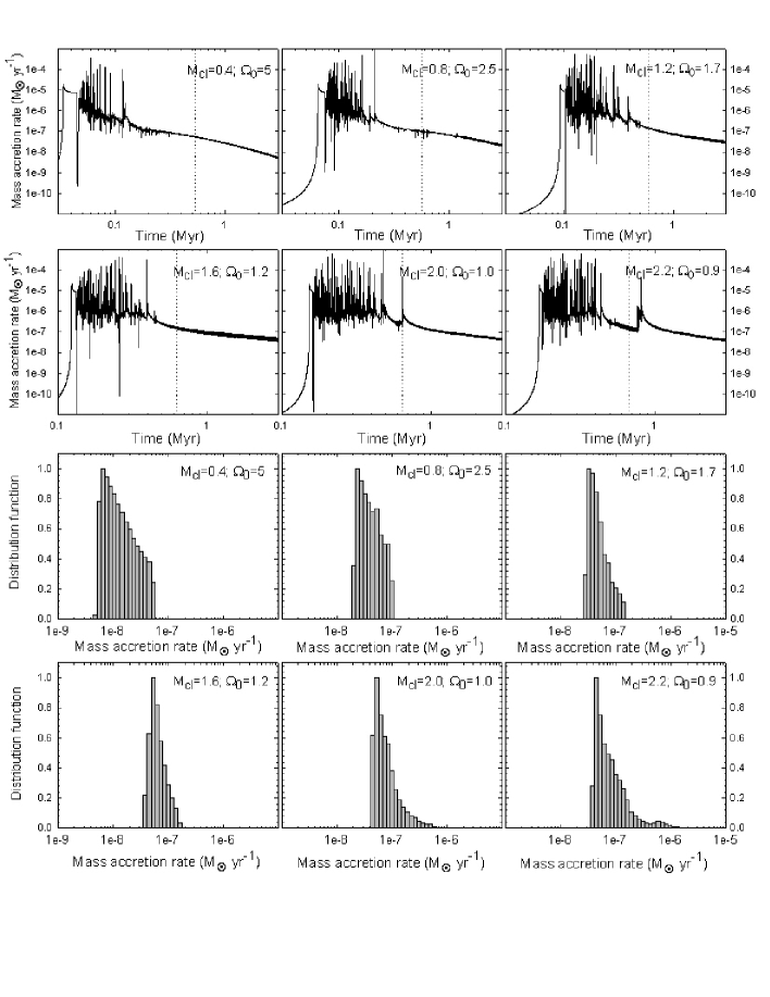
Figure 1.— Two upper panels. Mass accretion rates versus time elapsed since the beginning of simulations. Six models from model set 6 are presented, the initial cloud core mass $M_{\rm cl}$ (in $M_{\odot}$) and central angular velocity $\Omega_{0}$ (in km s^-1 pc^-1) are indicated in every panel. Vertical dotted lines mark the onset of the late accretion phase at 0.5 Myr from the central object formation. Two lower panels. Theoretical distribution functions (DFs) of accretion rates for the same six models showing the normalized number of accretion “measurements” as a function of the mass accretion rate. The measurements are done every 20 yr between 0.5 Myr and 3.0 Myr from the central object formation.

The early accretion history for all objects is similar—$\dot{M}$ reaches a peak value of $\sim 2.0\times 10^{-5}~{}M_{\odot}$ yr^-1 soon after the central object formation and settles at a near constant value of $\sim 10^{-5}~{}M_{\odot}$ yr^-1. Then, a transient sharp decline in $\dot{M}$ follows, manifesting the onset of disk formation. For a short time, centrifugal forces balance those of viscosity and gravity and the mass accretion rate drops to a negligible value. As the disk continues to build up its mass, the burst mode of accretion ensues. During this phase, prolonged periods of relatively low accretion at $10^{-7}$–$10^{-6}~{}M_{\odot}$ yr^-1 are interspersed with short episodes of activity when $\dot{M}$ increases to $10^{-4}$–$10^{-3}~{}M_{\odot}$ yr^-1. These accretion bursts are associated with disk fragmentation and formation of dense massive clumps that are later driven onto the central star due to the gravitational interaction with spiral arms (Vorobyov & Basu, 2006). Figure 1 demonstrates that the intensity and duration of the burst mode increases along the line of increasing cloud core masses. Most of the burst activity is constrained to the early several hundred thousand years of evolution, though the most massive objects can undergo a few bursts even after 0.5 Myr. In this late evolution phase, the mass accretion rates show a moderate decline by roughly one order of magnitude during 2–3 Myr. Some short-term variability is also present, but its magnitude is much smaller than that of the long-term decline.

Mass accretion rates in other model sets show a similar pattern of behavior. We now turn to comparing our numerically derived accretion rates in the late evolution phase with those inferred from observations.

3.2. Mass Accretion Rates

In this section, we compare our model mass accretion rates and central object masses with those compiled by Muzerolle et al. (2005, and references therein) for TTSs and BDs of age 0.5–3.0 Myr based on the measurements in (mostly) Taurus and other star formation regions. In order to facilitate the comparison, we time-average our model mass accretion rates and central object masses between 0.5 Myr and 3.0 Myr from the central object formation to obtain characteristic mean values $\langle\dot{M}\rangle$ and $\langle M_{\ast}\rangle$, respectively. For each model in Figure 1, we also construct the distribution function (DF) of accretion rates by calculating $\dot{M}$ every 20 yr between 0.5 Myr and 3.0 Myr from the central object formation and distributing the resulted values among 100 logarithmically-spaced bins in the $10^{-9}~{}M_{\odot}$ yr^-1–$10^{-5}~{}M_{\odot}$ yr^-1 range. The resultant DFs representing the normalized number of accretion “measurements” $N_{\dot{\rm M}}$ (by analogy to observations) in a given mass accretion bin are shown in two bottom rows of Figure 1. It is seen that the accretion rates in each model are localized in a specific interval. There is a preference for lower values of $\dot{M}$ in each interval, implying the measurements of mass accretion rates may be biased towards lower values.

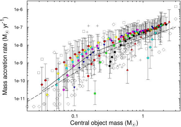
Figure 2.— Mass accretion rates versus central object masses. The open diamonds represent measurements of TTSs and BDs from Muzerolle et al. (2005, and references therein); the open squares and plus signs represent the confirmed detections and upper limits, respectively, compiled by Natta et al. (2006). The filled color symbols show the time-averaged mass accretion rates $\langle\dot{M}\rangle$ versus time-averaged central object masses $\langle M_{\ast}\rangle$ obtained in our numerical modeling. Each symbol type represents a distinct set of models with a constant value of $\beta$, as detailed in Table 1. In particular, model set 1 is plotted by cyan diamonds, model set 2—by red triangles-up, model set 3—by black circles, model set 4—by green squares, model set 5—by red circles, model set 6—by blue triangles-down, model set 7—by pink circles, model set 8—by cyan circles, model set 9—by yellow circles, and model set 10—by red diamonds. The bars represent typical variations in accretion rates in each model. The solid/dashed lines are the least-squares best fits to the model/observational data, respectively. In particular, the left lines are the fits to BDs and low-mass TTSs and right lines are the fits to the intermediate- and upper-mass TTSs.

Color symbols in Figure 2 represent the time-averaged mass accretion rates $\langle\dot{M}\rangle$ (in $M_{\odot}$ yr^-1) versus time-averaged object masses $\langle M_{\ast}\rangle$ (in $M_{\odot}$). Each filled symbol (of same color and shape) within a given set of models represents an individual object, which has formed from a cloud core of distinct mass, angular velocity, and size. In addition, each filled symbol is assigned vertical bars showing typical variations in the accretion rate between 0.5 Myr and 3.0 Myr after the central object formation. The typical variations are defined as mass accretion rates with $N_{\rm\dot{M}}$ equal to or greater than 0.05. This procedure helps to exclude objects with accretion rates that have a probability to be detected that is less than one part in twenty and are thus statistically insignificant. Considering the number ($\lesssim 20$) of detected objects along the line of constant central object mass, we believe that our typical variations represent conservative estimates. The open symbols and plus signs in Figure 2 represent data obtained from observations. In particular, the open diamonds represent measurements, mostly in Taurus, that have been compiled by Muzerolle et al. (2005, and references therein); the open squares represent detections in $\rho$ Oph obtained by Natta et al. (2006) and plus signs represent their upper limits to nondetections. We have excluded objects in the compilation of Muzerolle et al. (2005) that were later observed by Natta et al. (2006).

There are several important conclusions that can be drawn by analyzing Figure 2.

1. Our numerical models yield mass accretion rates that are of correct magnitude to explain the observed values in TTSs and BDs. There are only a few objects whose accretion rates fall beyond our predicted limits, but these objects can easily be accounted for by increasing $\beta$ marginally above our adopted values.

2. The time-averaged mass accretion rates and stellar masses for objects from every individual set of models form a unique track. These tracks are distinct for BDs and low-mass TTSs but tend to converge for upper-mass TTSs. Objects within each individual track have formed from cloud cores of distinct mass. In particular, objects in the lower-left end of the track have formed from cloud cores of lower mass.

3. Our models suggest that TTSs of 0.5–3.0 Myr age may have a wider range of mass accretion rates than implied from observations. In particular, we predict the existence of TTSs with accretion rates a factor of 10 lower than has been found in the compilation of Muzerolle et al. (2005, and references therein). The lack of such objects in the observational data is most likely explained by a difficulty to measure extremely low accretion rates in TTSs.

4. A dearth of BDs with accretion rates $\dot{M}>10^{-8}~{}M_{\odot}$ yr^-1 is likely caused by the lack of cloud cores with sufficiently large rotation rates. For instance, in order to reproduce the largest detected $\dot{M}$ in BDs ($\approx 10^{-8}~{}M_{\odot}$ yr^-1), we had to employ models with $\beta=0.032$. This ratio of the rotational to gravitational energy, according to Caselli et al. (2002), is close to the upper measured limit for dense cloud cores.

Perhaps, the most important conclusion from our modeling is that the observed scatter in the mass accretion rates along the line of equal object masses cannot be explained by intrinsic variability (shown in Figure 2 by vertical bars). This variability can account only for a maximum of two orders of magnitude scatter (with the noticeable exception of a few low-mass BDs) and often even less, but the measured rates typically span a range of three orders of magnitude. Figure 2 clearly demonstrates that some object-to-object variations are necessary to explain the observed scatter. This confirms previous claims by Natta et al. (2004) and Nguyen et al. (2009).

The object-to-object variations in the mass accretion rate along the line of equal (sub)stellar masses are caused by the difference in the disk masses. More massive disks are expected to drive higher rates of accretion (Vorobyov & Basu, 2008). Figure 2 shows that objects with greater $\langle\dot{M}\rangle$ but equal $\langle M_{\ast}\rangle$ belong to model sets characterized by greater values of $\beta$. At the same time, $\beta$ controls the disk mass because the centrifugal radius is directly proportional to $\beta$ (see Section 2.2). This means that models with greater $\beta$ (and greater $\langle\dot{M}\rangle$) but equal $\langle M_{\ast}\rangle$ are generally expected to harbor more massive disks and this is confirmed by our calculations of disk masses presented in Vorobyov (2009).

When all observational data in Figure 2 for TTSs and BDs are taken together, a least squares fit is described by a power law

$$\dot{M}=10^{-7.7}M_{\ast}^{1.8\pm 0.1}.$$ (9)

When we take the least-squares fit to the confirmed detections only (excluding non-detections represented by plus signs), we obtain the relation

$$\dot{M}=10^{-7.5}M_{\ast}^{2.0\pm 0.1}.$$ (10)

The difference between the best fits is not significant, but it demonstrates that the exponent is sensitive to the way the data are handled and may actually change when more observational data become available.

The least-squares best fit to all model data shown in Figure 2 is described by the relation

$$\langle\dot{M}\rangle=10^{-7.3}\langle M_{\ast}\rangle^{1.8\pm 0.1}.$$ (11)

It is evident that our numerical modeling can reproduce the observed relation reasonably well, except probably for the fact that we somewhat overestimate the observed rates. Possible reasons for this small discrepancy are discussed in Section 4.

However, we believe that taking a best fit over the whole mass range of BDs and TTSs may be misleading. In our previous paper (Vorobyov & Basu, 2008), we reanalyzed the data obtained from observations and argued that the exponent $n$ in the $\dot{M}\propto M_{\ast}^{n}$ relation takes different values for the lower-mass and upper-mass objects. In particular, we found $n=2.3\pm 0.6$ for BDs and low-mass TTSs with $M_{\ast}<0.25~{}M_{\odot}$, and $n=1.3\pm 0.3$ for intermediate- and upper mass TTSs with $0.25~{}M_{\odot}<M_{\ast}<3.0~{}M_{\odot}$. Two possible explanations were put forward for this apparent bimodality: variations in the observational methods and different mechanisms responsible for accretion. In this paper we focus on the latter alternative.

The left and right solid lines in Figure 2 are the least-squares fits to our model data for the lower- and upper-mass objects, respectively. The dashed lines are the corresponding best fits to the observational data. The least-squares fits in each mass regime are distinct and are described by the following power laws.
Modeling:

$$\left\{\begin{array}[]{ll}\langle\dot{M}\rangle=10^{-6.3}\,\langle M_{\ast}\rangle^{2.9\pm 0.5}&\,\,\mbox{if \,$\langle M_{\ast}\rangle<0.2~{}M_{\odot}$, }\\ \langle\dot{M}\rangle=10^{-7.3}\,\langle M_{\ast}\rangle^{1.5\pm 0.1}&\,\,\mbox{if \,$0.2~{}M_{\odot}\leq\langle M_{\ast}\rangle<3.0~{}M_{\odot}$ }.\end{array}\right.$$ (12)

Observations:

$$\left\{\begin{array}[]{ll}\dot{M}=10^{-7.2}\,M_{\ast}^{2.3\pm 0.6}&\,\,\mbox{if \,$M_{\ast}<0.2~{}M_{\odot}$, }\\ \dot{M}=10^{-7.6}\,M_{\ast}^{1.3\pm 0.3}&\,\,\mbox{if \,$0.2~{}M_{\odot}\leq M_{\ast}<3.0~{}M_{\odot}$ }.\end{array}\right.$$ (13)

It is evident that our numerical modeling corroborates the presence of bimodality in the observed $\dot{M}$–$M_{\ast}$ relation, though predicting a steeper dependence of $\dot{M}$ on $M_{\ast}$ for BDs and low-mass TTSs. We note, however, that a shallower dependence in the low-mass regime could be obtained by expanding our modeled range of values of $\beta$.

4. Discussion

How can different values of $\alpha$ affect our model accretion rates shown in Figures 1 and 2? Let us first focus on the intermediate- and upper mass TTSs with $0.2~{}M_{\odot}\leq M_{\ast}<3.0~{}M_{\odot}$. T Tauri disks are unlikely to sustain $\alpha\gtrsim 0.1$ throughout the whole disk volume during a typical disk lifetime of 3–5 Myr. Such large values of $\alpha$ lead to a disk depletion and disappearance on time scales of less than 1 Myr (Vorobyov & Basu, 2009). The results of that study excludes large values of $\alpha$ and leaves us with $\alpha\leq 10^{-2}$ as the most probable range of values. The accretion rates in the $\alpha=0$ case were presented by Vorobyov & Basu (2008). The $\langle\dot{M}\rangle\propto\langle M_{\ast}\rangle^{n}$ relation in this case was found to have an exponent $n=1.7\pm 0.1$, which is similar to the value found in the present study (see Equation 12), but the values of $\langle\dot{M}\rangle$ were approximately a factor of 2 smaller than in the $\alpha=10^{-2}$ case. This means that the actual value of $\alpha$ will not dramatically change the mean mass accretion rates, as long as it is $\leq 10^{-2}$.

The effect of varying $\alpha$ in the BD and low-mass TTS regime is more difficult to assess. Circumstellar disks in this mass regime have a lower surface density (than disks around intermediate- and upper-mass TTSs) and hence are expected to be more MRI-active. On the other hand, we do not expect $\alpha$ to be equal to or greater than $0.1$ due to the same reasons as discussed above. The fact that the least-squares fits to the model and observational data in Figure 2 tend to converge at the low-mass end implies that $\alpha=0.01$ is likely to be a good choice, certainly for the BD mass regime. The limit of small $\alpha\lesssim 10^{-3}$ is difficult to examine due to numerical reasons. Normally, as in the case of intermediate- and upper-mass TTSs, disks are relatively massive and artificial viscosity torques are much smaller than gravitational ones (Vorobyov & Basu, 2007). However, when both $\alpha$ and disk masses are small, artificial viscosity torques may become comparable to both gravitational and viscous ones. In addition, the imperfections at the inner inflow boundary could also introduce some low amplitude noise in the inner regions, which may not be negligible in the limit of small $\alpha$ and small disk masses. In this situation, the model mass accretion rates may be artificially overestimated. To avoid these complications, we decided to use $\alpha=10^{-2}$ in our modeling.

In the early disk evolution at $t<0.5$ Myr from the central star formation, gravitational-instability-induced torques dominate viscous ones, for intermediate and upper-mass TTSs (see e.g. Vorobyov & Basu, 2009), and this can influence considerably the subsequent time behavior of the system. We illustrate this phenomenon in Figure 3, which shows time-averaged mass accretion rates $\langle\dot{M}\rangle$ versus time-averaged central object masses $\langle M_{\ast}\rangle$ for model set 3 (top) and model set 6 (bottom). Every model in these sets is run twice: first time—with both disk self-gravity and viscosity and second time—with disk viscosity only. In the latter case, the disk self-gravity is artificially set to zero, thus nullifying the gravitational instability as well, but the gravity of the central object is kept. The open squares in Figure 3 show the data obtained in models with both disk self-gravity and viscosity (these data are identical to those shown in Figure 2), while the filled squares present the data for models with disk viscosity only.

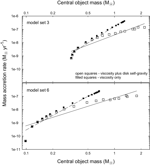
Figure 3.— Time-averaged mass accretion rates $\langle\dot{M}\rangle$ versus time-averaged central object masses $\langle M_{\ast}\rangle$ for all models from model set 3 (top) and model set 6 (bottom). Open squares show the case when both disk self-gravity and viscosity are at work, while filled squares correspond to the case when disk self-gravity is set to zero and viscosity remains the only mass transport agent in the disk. The solid and dashed lines are the least-squares best fits to models with disk self-gravity and without disk self-gravity, respectively.

It is evident that gravitational instability has little effect on the low-mass objects in each model set, but its effect becomes noticeable along the line of increasing object masses. Starting from the fourth or fifth least massive object in each set, the models without disk self-gravity begin to yield an $\langle\dot{M}\rangle$ that is greater than those of self-gravitating models, while at the same time underestimating the central object mass $\langle M_{\ast}\rangle$. In general, models without self-gravity tend to produce stars with masses that are too low and mass accretion rates that are too high. This effect may seem counterintuitive since both viscous and gravitational torques are expected to act together to increase $\langle\dot{M}\rangle$. However, it is important to keep in mind that our time-averaged mass accretion rates apply to the late evolution phase between 0.5 Myr and 3.0 Myr after the formation of the protostar. In contrast, during the early phase ($<0.5$ Myr), the time-averaged mass accretion rates in models with self-gravity are greater than in models without self-gravity. This is due to vigorous gravitational instability that acts in self-gravitating disks. As a result, models with self-gravity build up the stellar mass and deplete the total gas reservoir much faster than models without self-gravity. This causes the mass accretion rate in self-gravitating disks to be lesser in the late evolution phase.

In order to better illustrate the difference in the mass accretion rates, we take the least-squares best fits to the models with self-gravity (solid lines) and models without self-gravity (dashed lines). In the former case, we obtain exponents $n=2.5\pm 0.2$ (top panel, model set 3) and $n=2.1\pm 0.2$ (bottom panel, model set 6). When the least-squares fit is taken for both sets of models, we obtain $n=2.0\pm 0.2$. This is quite similar to the exponent found for the complete set of models (see eq. [11]). In the case without self-gravity, we obtain exponents $n=4.2\pm 0.2$ (top panel, model set 3) and $n=3.6\pm 0.2$ (bottom panel, model set 6), which are considerably larger than those for models with self-gravity. In this example, we have not considered all models due to an enormous computational load, but we do not expect this tendency to change considerably for the complete set of models. This allows us to conclude that if not for the disk self-gravity and associated gravitational instability in the early evolution phase, we would have had difficulty to recover the observed $\dot{M}$–$M_{\ast}$ relation.

Another important feature of the non-self-gravitating models in Figure 3 is an apparent lack of bimodality in the $\dot{M}$–$M_{\ast}$ relation. Almost all models within an individual set, except for a few ones with the smallest masses of the central object, fall onto a track that is well described by a straight line in log–log space. This strongly suggests that the bimodality is the result of gravitational instability acting in the early phase of disk evolution.

5. Conclusions

Using numerical hydrodynamic simulations of circumstellar disk formation and evolution, we have studied the mass accretion rates in BDs and TTSs, focusing mainly on the late evolution phase between 0.5 Myr and 3.0 Myr from the central object formation. Our numerical model involves both disk self-gravity, which is accurately computed via the solution of the Poisson integral, and turbulent viscosity, the latter being described by a usual Shakura & Sunyaev parameterization with the $\alpha$-parameter set to $10^{-2}$. The theoretical data are compared against those obtained from the measurements in young star-forming clusters Muzerolle et al. (2005, and references therein). We find the following.

• Our numerical modeling of self-consistently-formed circumstellar disks yields mass accretion rates of correct magnitude to explain the observed values in TTSs and BDs of 0.5–3.0 Myr age.

• We corroborate our previous conclusion (Vorobyov & Basu, 2008) that the dependence of the mass accretion rates ($\dot{M}$) on the central object mass ($M_{\ast}$) in TTSs and BDs can be better described by a bimodal power-law function rather than that with a single exponent. Mass accretion rates of BDs and low-mass TTSs ($M_{\ast}<0.2~{}M_{\odot}$) have a steeper dependence on $M_{\ast}$ than those of the intermediate- and upper-mass TTSs ($0.2~{}M_{\odot}\leq M_{\ast}<3.0~{}M_{\odot}$). In particular, the least-squares fits to our model data yield exponents $n=2.9\pm 0.5$ and $n=1.5\pm 0.1$ for the objects with mass $M_{\ast}<0.2~{}M_{\odot}$ and $0.2~{}M_{\odot}\leq M_{\ast}<3.0~{}M_{\odot}$, respectively. The corresponding fits to the observational data produce exponents $n=2.3\pm 0.6$ and $n=1.3\pm 0.3$.

• The apparent bimodality in the $\dot{M}$–$M_{\ast}$ relation is caused by vigorous gravitational instability in the early phase of disk evolution. The gravitational instability serves to limit disk masses in the intermediate and upper-mass TTSs (Vorobyov, 2009), thus effectively setting an upper limit on the mass accretion rates in the late evolution and flattening the $\dot{M}$–$M_{\ast}$ relation in this mass regime. Models without self-gravity greatly overestimate the observed mass accretion rates, while at the same time underestimating the central object masses. As a result, the non-self-gravitating models fail to account for the observed $\dot{M}$–$M_{\ast}$ relation, predicting a much steeper dependence of $\dot{M}$ on $M_{\ast}$.

• The observed large scatter in mass accretion rates along the line of equal (sub)stellar masses is caused in part by the intrinsic variability during the evolution of individual objects, which may span a range of one (intermediate- and upper-mass TTSs) to two (BDs and low-mass TTSs) orders of magnitude. The other part is object-to-object variations due to different initial conditions. Our conclusion is in agreement with that of Natta et al. (2004) and Nguyen et al. (2009) based on the analysis of variability in TTSs.

• We predict the existence of TTSs with accretion rates a factor of 10 lower than those reported by Muzerolle et al. (2005, and references therein). Our modeling also indicates that upper mass TTSs may exhibit a few FU-Ori-like outbursts with accretion rates greater than $10^{-5}~{}M_{\odot}$ yr^-1. However, the anticipated number of such peculiar objects is quite small and they are not expected to break the existing $\dot{M}$–$M_{\ast}$ relation.

References

- Armitage et al. (2001) Armitage, P. J., Livio, M., & Pringle, J. E. 2001, MNRAS, 324, 705
- Basu (1997) Basu, S. 1997, ApJ, 485, 240
- Basu (1998) Basu, S. 1998, ApJ, 509, 229
- Cai et al. (2008) Cai, K., Durisen, R. H., Boley, A. C., Pickett, M. K., & Mejía, A. C. 2008, ApJ, 673, 1138
- Calvet et al. (2004) Calvet, N., Muzerolle, J., Briceño, C., Hernández, J., Hartmann, L., Sauceno, J. L., & Gordon, K. D. 2004, AJ, 128, 1294
- Caselli et al. (2002) Caselli, P., Benson, P. J., Myers, P. C., & Tafalla, M. 2002, ApJ, 572, 238
- D’Alessio et al. (1999) D’Alessio, P., Calvet, N., Hartmann, L., Lizano, S., & Cantó, J. 1999, ApJ, 527, 893
- Goodwin et al. (2002) Goodwin, S. P., Ward-Thompson, D., & Whitworth, A. P. 2002, MNRAS, 330, 769
- Hartmann et al. (2006) Hartmann, L., D’Alessio, P., Calvet, N., & Muzerolle, J. 2006, ApJ, 648, 484
- Jones et al. (2001) Jones, C. E., Basu, S., & Dubinski, J. 2001, ApJ, 551, 387
- Jones & Basu (2002) Jones, C. E., & Basu. S. 2002, ApJ, 569, 280
- Kratter et al. (2008) Kratter, K. M., Matzner, C. D., & Krumholz, M. R. 2008, ApJ, 681, 375
- Mohanty et al. (2005) Mohanty, S., Jayawardhana, R., & Basri, G. 2005, ApJ, 626, 498
- Muzerolle et al. (2003) Muzerolle, J., Hillenbrand, L., Calvet, N., Briceño, C., & Hartmann, L. 2003, ApJ, 592, 266
- Muzerolle et al. (2005) Muzerolle, J., Luhman, K., Briceño, C., Hartmann, L., & Calvet, N. 2005, ApJ, 625, 906
- Natta et al. (2004) Natta, A., Testi, L., Muzerolle, J., Randich, S., Comer on, F., & Persi, P. 2004, A&A, 424, 603
- Natta et al. (2006) Natta, A., Testi, L., & Randich, S. 2006, A&A, 452, 245
- Nguyen et al. (2009) Nguyen, D. C., Scholz, A., van Kerkwijk, M. H., Jayawardhana, R., Brandeker, A. 2009, ApJ, 694, L153
- Shakura & Sunyaev (1973) Shakura, N. I., & Sunyaev, R. A. 1973, A&A, 24, 337
- Tassis (2007) Tassis, K. 2007, MNRAS, 379, L50
- Vorobyov (2009) Vorobyov, E. I. 2009, ApJ, 692, 1609
- Vorobyov & Basu (2005) Vorobyov, E. I., & Basu, S. 2005, ApJ, 633, L137
- Vorobyov & Basu (2006) Vorobyov, E. I., & Basu, S. 2006, ApJ, 650, 956
- Vorobyov & Basu (2007) Vorobyov, E. I., & Basu, S. 2007, MNRAS, 381, 1009
- Vorobyov & Basu (2008) Vorobyov, E. I., & Basu, S. 2008, ApJ, 676, 139
- Vorobyov & Basu (2009) Vorobyov, E. I., & Basu, S. 2009, MNRAS, 393, 822
- Zhu et al. (2009) Zhu, Z., Hartmann, L. & Gammie, C. F. 2009, ApJ, 694, 1045