Phase diagram of an anisotropic frustrated ferromagnetic spin-$\frac{1}{2}$ chain in a magnetic field: a density matrix renormalization group study

Abstract

We study the phase diagram of a frustrated spin-1/2 ferromagnetic chain with anisotropic exchange interactions in an external magnetic field, using the density matrix renormalization group method. We show that an easy-axis anisotropy enhances the tendency towards multimagnon bound states, while an easy-plane anisotropy favors chirally ordered phases. In particular, a moderate easy-plane anisotropy gives rise to a quantum phase transition at intermediate magnetization. We argue that this transition is related to the finite-field phase transition experimentally observed in the spin-1/2 compound LiCuVO₄.

I Introduction

The interplay of frustration and quantum fluctuations in reduced dimensions often leads to unconventional magnetic order, such as chiral or spin-nematic states (see, e.g., Refs. Villain78, ; AndreevGrishchuk84, ; chubukov91a, ; nersesyan98, ; kaburagi99, ; kolezhuk00, ; hikihara01, ; lecheminant01, ; kolezhuk05, ; laeuchli06, ; vekua07, ; mcculloch08, ; hikihara08, ; okunishi08, ; sudan09, ). A particularly simple model yet realizing a fascinating variety of competing phases is the frustrated ferromagnetic spin-$1/2$ chain in the presence of an external magnetic field,hm06a ; vekua07 ; kecke07 ; hikihara08 ; sudan09 described by the Hamiltonian

$$\mathcal{H}=\sum_{l}\Big{\{}J_{1}(\bm{S}_{l}\cdot\bm{S}_{l+1})_{\Delta}+J_{2}(\bm{S}_{l}\cdot\bm{S}_{l+2})_{\Delta}-hS_{l}^{z}\Big{\}},$$

$$(\bm{S}_{1}\cdot\bm{S}_{2})_{\Delta}\equiv S_{1}^{x}S_{2}^{x}+S_{1}^{y}S_{2}^{y}+\Delta S_{1}^{z}S_{2}^{z},$$ (1)

where $\bm{S}_{l}$ is a spin-$\frac{1}{2}$ operator acting at site $l$, $J_{1}<0$ and $J_{2}>0$ are the nearest and next-nearest neighbor exchange constants, $h$ is the external magnetic field, and $\Delta$ is the exchange anisotropy. The system may be alternatively viewed as two antiferromagnetic chains coupled by a ferromagnetic zigzag-type coupling whose strength is measured by the frustration parameter

$$\beta=J_{1}/J_{2}.$$ (2)

The isotropic ($\Delta=1$) version of this model has a rich magnetic phase diagram exhibiting states with different types of competing unconventional orders.hm06a ; vekua07 ; kecke07 ; hikihara08 ; sudan09 In particular, the vector chirality, being the quantum remnant of the classical helical spin order, competes with multipolar orders which characterize the pseudo-condensate consisting of multimagnon bound states. A similar effect has been previously predictedkolezhuk05 and recently confirmed numericallymcculloch08 ; okunishi08 for the case of the antiferromagnetic frustrated chain with $J_{1}>0$, $J_{2}>0$.

The vector chirality (spin current) $\bm{\kappa}_{l}=(\bm{S}_{l}\times\bm{S}_{l+1})$ can, even in one dimension, exhibit true long-range order (LRO), i.e., the asymptotic value $\kappa_{0}^{2}=\lim_{|n-n^{\prime}|\to\infty}C_{\kappa}(n,n^{\prime})$ of the chirality correlator

$$C_{\kappa}(n,n^{\prime})=\langle\kappa_{n}^{z}\kappa_{n^{\prime}}^{z}\rangle$$ (3)

can be finite. In the presence of an external magnetic field or of a finite anisotropy $\Delta\not=1$, the rotational $SU(2)$ symmetry is broken down to $U(1)\times Z_{2}$, and the vector chiral order corresponds to the spontaneous breaking of the discrete $Z_{2}$ (parity) symmetry. At a finite magnetization, the presence of a nonzero vector chirality automatically leads to the emergence of scalar chirality,Al-Hassanieh+09 defined as a mixed product of three spins on a triangular plaquette. It has been shown recently Bulaevskii+08 that in the underlying electronic system the presence of a scalar chirality always induces charge currents, leading to orbital antiferromagnetism.

A common feature of the multipolar phases is that the excitations that correspond to a single spin flip (i.e., to a change $\Delta S^{z}=\pm 1$ of the $z$-component of the total spin) are gapped, and therefore, the in-plane spin correlator $\langle S^{+}_{n}S^{-}_{n^{\prime}}\rangle$ decays exponentially with the distance $|n-n^{\prime}|$. This distinguishes such phases from the usual spin fluid phases (also called the XY1-type, in the classification due to SchulzSchulz86 ) where the $\langle S^{+}_{n}S^{-}_{n^{\prime}}\rangle$ correlations decay algebraically. At the same time, the excitations with $\Delta S^{z}=\pm 2$ are gapless in the quadrupolar phase, those with $\Delta S^{z}=\pm 3$ are gapless in the octupolar phase, etc. The long-range quadrupolar (nematic) order, characterized by the finite asymptotic value of the correlator

$$C_{2}(n,n^{\prime})=\langle S^{+}_{n}S^{+}_{n+1}S^{-}_{n^{\prime}}S^{-}_{n^{\prime}+1}\rangle$$ (4)

at $|n-n^{\prime}|\to\infty$, would break the $U(1)$ symmetry, such that those correlations can only be quasi-long-range (i.e., exhibiting a power-law decay) in purely one-dimensional (1D) systems, yet they may develop into a true LRO in real materials where a finite three-dimensional interaction is always present. The same applies to the higher multipolar order parameters such as the octupolar (triatic) order defined by the correlator of the type $C_{3}(n)=\langle S^{+}_{l}S^{+}_{l+1}S^{+}_{l+2}S^{-}_{l+n}S^{-}_{l+n+1}S^{-}_{l+n+2}\rangle$, etc. Finally, the spin density correlator

$$C_{\rm SDW}(n,n^{\prime})=\langle S^{z}_{n}S^{z}_{n^{\prime}}\rangle-\langle S^{z}_{n}\rangle\langle S^{z}_{n^{\prime}}\rangle$$ (5)

has a power-law decay in multipolar phases (as well as in the other phases mentioned above), and depending on the dominant correlations, a multipolar phase can be further characterized as being of the nematic (triatic, etc.) or spin-density wave (SDW) type.

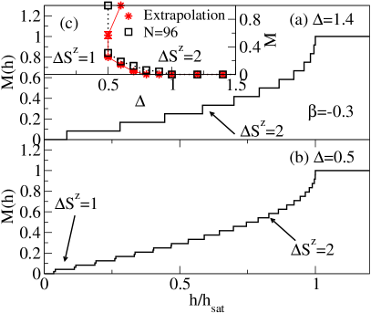
Figure 1: (Color online) (a) and (b) Magnetization curves for $\beta=-0.3$ and (a) $\Delta=1.4$ and (b) $\Delta=0.5$. (c) Phase boundaries in the $M$ vs $\Delta$ plane, based on $M(h)$, for $\beta=-0.3$ (squares: $N=96$; stars: extrapolation in $1/N$).

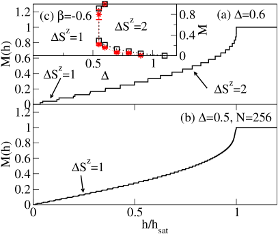
Figure 2: (Color online) (a) and (b) Magnetization curves for $\beta=-0.6$ and (a) $\Delta=0.6$ and (b) $\Delta=0.5$. (c) Phase boundaries in the $M$ vs $\Delta$ plane, based on $M(h)$, for $\beta=-0.6$ (squares: $N=96$; stars: extrapolation in $1/N$).

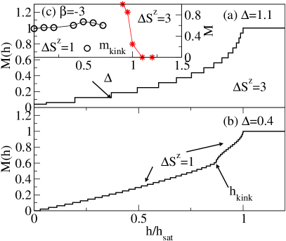
Figure 3: (Color online) (a) and (b) Magnetization curves for $\beta=-3$ and (a) $\Delta=1.1$ and (b) $\Delta=0.4$. The arrow in (a) indicates the location where the magnetization starts to increase in steps of $\Delta S^{z}=3$. (c) Phase boundaries in the $M$ vs $\Delta$ plane, based on $M(h)$, for $\beta=-3$ (extrapolated in the system size $N\to\infty$).

In the isotropic model at small $|\beta|$ the spin gap is predicted to be either zeroWhiteAffleck96 ; AllenSenechal97 or astronomically small.ItoiQin01 The zero-field phase diagram of the frustrated ferromagnetic chain with an anisotropic exchange has been studied, both for the case of anisotropic nearest-neighbor interactions onlyplekhanov08 ; avella08 and for the case in which both exchange paths exhibit the same anisotropy.somma01 ; dmitriev08 ; dmitriev09 ; furukawa08 For the latter example, relevant to our work, the existence of dimer, spin fluid, and (anti)ferromagnetically ordered phases has been suggested.somma01 Moreover, a chirally ordered phase has been predicted to exist at $|\beta|\lesssim 1$ for $\Delta<1$.furukawa08

The model (I) has been suggested to be relevant for the description of several recently discovered quasi one-dimensional magnetic materials such as LiCuVO₄ (Ref. enderle05, ), Rb₂Cu₂Mo₃O₁₂ (Ref. hase04, ), Li₂ZrCuO₄ (Ref. drechsler07, ), and anhydrous $\rm CuCl_{2}$ (Ref. banks+09, ).

Our goal is to study the interplay between the exchange anisotropy and the magnetic field as reflected in the magnetic phase diagram of the model (I). The motivation for our work stems from the experimental resultsenderle05 ; banks07 ; schrettle08 for LiCuVO₄ that have revealed the existence of a phase transition in a magnetic field from a helically ordered state at low field values into another phase at high magnetic fields where the magnetic order seems to be collinear and directed along the field axis.Buettgen+07 ; schrettle08 If one imagines “switching off” the three-dimensional interactions, the helical phase might get transformed either into the chirally ordered phase or into a usual spin-fluid XY phase (albeit with incommensurate spin correlations), while the unknown high-field phase could correspond to the quadrupolar state of the purely 1D model.

However, for the specific parameter values suggested to be relevant for this particular material, i.e., $\beta\approx-0.3$, the 1D model (I) with isotropic interactions ($\Delta=1$) does not support any phase transitions at intermediate field values.hm06a ; banks07 Numerical resultshikihara08 ; sudan09 for $|\beta|>1$ suggest that the vector chiral phase shrinks very fast with decreasing $|\beta|$, and thus it is hardly detectable already at $\beta\simeq-1$. Although one might assume that the vector chiral phase still persists in an infinitesimally narrow region that vanishes asymptotically at $\beta\to 0$, this would not suffice to explain the finite-field transition in LiCuVO₄ occuring at a relatively high field strength of about 20% of the saturation field.banks07

At the same time, electron spin resonance experimentsVasilev+01 ; KrugVonNidda+02 indicate that the exchange interactions in LiCuVO₄ have an easy-plane anisotropy of about 10%. This puts forward a natural question whether including this type of an anisotropy may drive the sought-for phase transition. We show that this is indeed the case: there is a finite window of $\Delta<1$ where the spin fluid phase persists at low fields, while the quadrupolar-SDW state occupies the high-field region.

In the present study, we focus on parameter values relevant for LiCuVO₄ (Ref. enderle05, ), anhydrous $\rm CuCl_{2}$ (Ref. banks+09, ), and Rb₂Cu₂Mo₃O₁₂ (Ref. hase04, ), namely $\beta=-0.3$, $-0.6$ and $-3$, respectively. To carry out the numerical analysis, we employ the density matrix renormalization group (DMRG) method,white92b ; white93 ; schollwoeck05 and our study is mainly based on the calculation of magnetization curves $M=M(h)$ and the chiral order parameter $\kappa_{0}$. In Sec. II, we present the analysis of magnetization curves $M=M(h)$ as a function of the exchange anisotropy $\Delta$. From the magnetization curves, we are able to extract the phase boundaries. The results of the magnetization curves analysis are further supported and supplemented by the analysis of correlations presented in Sec. III. Our main result, the magnetic phase diagrams derived from the combined analysis of magnetization curves and correlations functions, is presented in Sec. IV. We conclude with a summary and discussion in Sec. V.

II Magnetization curves

In this Section, we present magnetization curves of the ferromagnetic frustrated chain and discuss their relation to the phase boundaries of the model (I) in the magnetization vs anisotropy plane. To that end, we compute the ground-state energies $E_{0}(S^{z})$ for all values $S^{z}=\sum_{l}S^{z}_{l}$ of the $z$-component of the total spin. By subtracting the Zeeman energy $-hS^{z}$ and carrying out the Maxwell construction, we find, for each given field $h$, the quantum number $S^{z}$ and respectively the magnetization $M=2S^{z}/N$ of the ground state, where $N$ is the number of sites. Typically, we use about $m=600$ DMRG states, and open boundary conditions.

Our results for $\beta=-0.3$, $-0.6$, and $-3$ are shown in Figs. 1, 2, and 3, respectively. For both $\beta=-0.3$ and $\beta=-0.6$, at $\Delta=1$ the system is in the quadrupolar phaseokunishi03 ; hm06a ; banks07 (also called “even-odd”,okunishi03 or XY2 phase in the classification by SchulzSchulz86 ): the magnetization increases in steps of $\Delta S^{z}=2$, due to the presence of two-magnon bound states. In this phase, the $\Delta S^{z}=2$ sector, corresponding to the simultaneous flip of two spins, is gapless, while single-spin excitations with $\Delta S^{z}=1$ are gapped.vekua07 In terms of correlation functions, at small fields the leading instability is in the SDW channel, while at high fields the quadrupolar (nematic) correlations of the type (4) dominate.chubukov91a ; vekua07

The results of Figs. 1 and 2 show that an easy-axis anisotropy $\Delta>1$ simply stabilizes the $\Delta S^{z}=2$ phase [see, e.g., Fig. 1(a)].note1 In contrast to that, an easy-plane anisotropy, $\Delta<1$, disfavors the formation of two-magnon bound states and eventually, we observe the disappearance of the $\Delta S^{z}=2$ region [see Figs. 1(b), 2(a) and 2(b)], giving room to the phase with $\Delta S^{z}=1$. In Sec. III, we will see that this region exhibits chiral order. The results of the analysis of $M(h)$ for $|J_{1}|<J_{2}$ are summarized in Figs. 1(c) and 2(c): in both cases, below $\Delta\lesssim 0.5$, the quadrupolar phase has disappeared. It is worthwhile to remark that in the case of a weak coupling ($\beta=-0.6$ and $\beta=-0.3$), we observe a reentrant behavior in the vicinity of $\Delta\sim 0.55$: as the magnetization increases, one starts in the $\Delta S^{z}=1$ region, then enters into the quadrupolar phase, and reenters into the $\Delta S^{z}=1$ one at $M\approx 0.75$. As we shall see below, this picture is also supported by the behavior of the chirality correlations.

In the vicinity of the saturation field ($M=1$) the position of the boundary of the quadrupolar phase is in good agreement with the analysis of Ref. KuzianDrechsler07, . According to Ref. KuzianDrechsler07, , the field $h_{s,2m}$ at which the two-magnon bound state gap closes is given by $h_{s,2m}/J_{2}=[1+(\Delta+1)^{2}-\Delta^{2}(1-\beta)^{2}]/[2(1-\beta\Delta)]$, while the respective value for one-magnon states is given by $h_{s,1m}/J_{2}=(\Delta-1)(1+\beta)+(4+\beta)^{2}/8$. Comparing those two fields, one finds, for example, that for $\beta=-0.3$ the instability of the fully polarized state at the saturation field is by condensation of the two-magnon bound states at $\Delta>\Delta_{s}\simeq 0.54$, and by one-magnon states below that value. The critical point $\Delta_{s}$ is only slightly dependent on the frustration $\beta$, e.g., at $\beta=-0.6$ one has $\Delta_{s}\simeq 0.58$.

Let us now turn to the regime of strong coupling, $\beta=-3$. In the isotropic case, the system is in a chiral phase at small magnetizations, and with increasing $M$ one enters a multipolar (actually, octupolar) phase.sudan09 This octupolar phase is characterized by $\Delta S^{z}=3$ steps in the magnetization curve,hm06a which indicates that three-magnon bound states are excitations with the lowest energy per unit of $\Delta S^{z}$. Similar to the $|\beta|<1$ case, an easy-axis anisotropy $\Delta>1$ stabilizes the $\Delta S^{z}=3$ multipolar phase. We illustrate this behavior in Fig. 3(a), showing the magnetization curve for $\Delta=1.1$. In the easy-plane region $\Delta<1$, the magnetization curve further exhibits a kink-like feature at about $M\sim 0.6$, as the example of $\Delta=0.4$, plotted in Fig. 3(b), shows. We trace this kink back to the incommensurability and the emergence of multiple Fermi points, following the reasoning of Refs. okunishi99, ; okunishi03, . The resulting phase diagram for $\beta=-3$, based on the $M(h)$ curves, is presented in Fig. 3(c).

Summarizing the results of this section, one can say that the main feature, common for all values of the frustration parameter $\beta$ considered here, is that an easy-plane anisotropy $\Delta<1$ gives rise to a mid-field phase transition from the $\Delta S^{z}=1$ “phase” at low fields to a multipolar ($\Delta S^{z}\geq 2$) phase at high fields. In Sec. III, we will further focus on characterizing the region with gapless triplet excitations (i.e., $\Delta S^{z}=1$) and show that it actually contains several different phases.

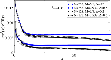
Figure 4: (Color online) Examples of the chirality correlation function $\langle\kappa^{z}(x)\kappa^{z}(0)\rangle$ at $\beta=-0.6$ for chains with $128$ and $256$ sites, for two fixed points in the $(\Delta,M)$ plane.

III Correlation functions

In this section, we study the correlation functions, complementing the analysis of the magnetization curves presented in the previous section. While the multipolar phases are most easily detected by the appearance of the $\Delta S^{z}>1$ steps in the $M(h)$ curves, the region corresponding to $\Delta S^{z}=1$ can actually contain several different phases. Indeed, the spin-fluid (XY1) phase of the easy-plane spin chain, described by the one-component Tomonaga-Luttinger (TL1) liquid, the two-component (TL2) spin-fluid phase,okunishi99 and the chirally ordered phase all have gapless excitations in the $\Delta S^{z}=\pm 1$ channel. Thus all those phases will show up as a single $\Delta S^{z}=1$ “phase” and cannot be further discerned from the $M(h)$ studies. Analyzing the chiral correlation function $C_{\kappa}(n,n^{\prime})$, we can identify the chiral phase, and the rest of the $\Delta S^{z}=1$ region can be divided into the TL1 and TL2 phases by the line where a kink occurs in the magnetization curve (see Sec. II).

Within the multipolar ($\Delta S^{z}=p\geq 2$) phases, an additional analysis of correlations is necessary to distinguish between the regions with dominant spin density wave correlations ($\rm SDW_{p}$-”phases”) and those with dominant multipolar (nematic, triatic, etc.) ones. Although the transitions between, e.g., $\rm SDW_{2}$ and nematic is only a crossover and not a true phase transition in our purely one-dimensional model, such an analysis can be helpful in understanding what could be the resulting order in a real material, where frustrated chains are coupled by a weak three-dimensional interaction.

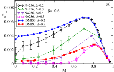
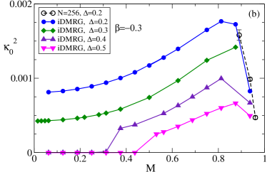
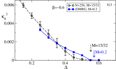
Figure 5: (Color online) Square of the vector chirality $\kappa_{0}^{2}$: (a) vs magnetization $M$ at $\beta=-0.6$ and various fixed values of the anisotropy $\Delta$; (b) the same at $\beta=-0.3$; (c) vs the anisotropy $\Delta$ at two fixed values of $M$ and $\beta=-0.6$ (the arrows here denote the respective positions of the $\Delta S^{z}=1$ phase boundary); (d) vs the frustration parameter $|\beta|=-J_{1}/J_{2}$ at fixed $\Delta=0.2$ and $M=0.703125$. Open symbols denote the finite-size DMRG results, and solid symbols correspond to iDMRG.

III.1 DMRG methods for the calculation of the vector chirality

Using the finite-size DMRG methodwhite93 ; schollwoeck05 in its matrix-product formulation,McCulloch07 we have studied correlators (3), (4), and (5) in chains of $N=256$ spins. This length has been chosen since, on the one hand, it is sufficiently large to study the asymptotic long-distance behavior of the correlations, and on the other hand, it is small enough to ensure that the DMRG calculation converges with a moderate number $m$ of representative states kept. The typical value of $m$ necessary to reach good convergence strongly depends on the frustration parameter $\beta=J_{1}/J_{2}$: while for $\beta=-3$, $m=400$ is normally sufficient, at smaller coupling ($\beta=-0.6$) this figure grows to $m\simeq 600$-$800$, and in the regime of weakly coupled chains ($\beta=-0.3$) one needs $m\simeq 800$-$1200$, even for large magnetizations $M\gtrsim 0.7$ where the convergence is generally faster. The correlators (3)-(5) have been calculated for a large number of ground states in sectors with different $S^{z}$. They have been averaged over the starting and final positions $n$, $n^{\prime}$, and contributions with $n$ or $n^{\prime}$ being closer as as a fixed “cutoff” (taken here to be $20$ sites) to the chain ends have been discarded. Typical chiral correlation functions are shown in Fig. 4. From such data we have extracted the asymptotic value of the correlator which corresponds to the square of the chirality $\kappa_{0}^{2}$.

A proper finite-size scaling analysis of chirality correlations is, however, hampered by strong boundary effectsmcculloch08 ; hikihara08 ; okunishi08 that tend to spoil the bulk correlations for smaller system sizes. Due to that, it becomes difficult to distinguish the chiral LRO from a non-chiral phase in those situations where the chiral order parameter $\kappa_{0}$ becomes very small. In such cases, we have complemented the finite-size DMRG study with another technique, namely, the recently proposediDMRG matrix-product formulation of the infinite-size DMRG algorithm (iDMRG) which allows to treat systems with finite magnetization (in contrast to the conventional infinite-size DMRG method, see, e.g., Ref. hikihara01, ). We utilize an algorithm with conserved $U(1)$ symmetry to constrain the average magnetization per unit cell. The convergence rate of iDMRG is essentially independent of the size of the unit cell, which can be arbitrarily large. The advantage of the iDMRG is that the scaling in $(m,N)$ is replaced by the scaling in the number of states $m$ alone, which can be translated into a scaling with respect to the correlation length via $\xi\sim m^{\eta}$, where the correlation length $\xi$ is determined from the next-leading eigenvalue of the transfer operator.criticalscaling For critical states described by a conformal field theory (CFT), $\eta$ is a function of the central charge.Pollmann The spectrum of the transfer operator also gives detailed information about the exponents and operator content of the CFT.IanInProgress

In the standard finite-size DMRG formulation, the degeneracy of two chirally ordered ground states will be lifted by finite-size corrections. Therefore the purely real ground state of a finite system is obtained as a superposition of states with $\pm\kappa_{0}$. The iDMRG,iDMRG in contrast, allows for a spontaneous breaking of the parity symmetry, which also breaks time reversal symmetry and leads to a complex valued wavefunction. This gives a transfer operator that is not Hermitian, but is instead complex-symmetric. The chirality order parameter can then be calculated just as $\kappa_{0}=\Im\langle S^{+}_{n}S^{-}_{n+1}\rangle$. The iDMRG randomly selects one of the two ground states, with $\kappa_{0}$ either positive or negative. For broken symmetry states the iDMRG is quite efficient, because the broken symmetry state requires fewer basis states than a superposition. For example, the representation of a superposition of the $\pm\kappa_{0}$ states in a form of a matrix product state requires precisely double the number of basis states, because the reduced density matrices of the two degenerate ground states have no overlap in the thermodynamic limit. In a finite-size calculation, the mixing of the two states leads to somewhat less than a factor 2 in the required basis size, nevertheless one still requires generally fewer states in iDMRG compared with its finite-size counterpart.

III.2 Vector chirality in the weak coupling regime ($|J_{1}|<J_{2}$)

The results for the weak coupling regime $|\beta|<1$ are shown in Fig. 5. One can see that the finite-size DMRG results give the impression that both at $\beta=-0.6$ and $\beta=-0.3$, the vector chiral LRO vanishes in the low-field part of the $\Delta S^{z}=1$ region. However, as mentioned above, we cannot reliably detect the presence of a very small chiral order with the finite-size DMRG method because of strong boundary effects. Applying the iDMRG technique, one can clearly see that the finite-size DMRG tends to underestimate the value of the chiral order parameter $\kappa_{0}$, cf. Fig. 5(a,b).note-errbars

As can be seen from Figs. 5(c) and (d), the magnitude of the chiral order parameter diminishes quickly when $|\beta|$ decreases, and also when one approaches the boundary of the $\Delta S^{z}=1$ region. The convergence in those cases becomes very slow. Figure 6 shows the convergence of the iDMRG method at a point close to the $\Delta S^{z}=1$ boundary: a finite chirality is detected when the largest intrinsic correlation length $\xi$ of the method exceeds 100 sites. Taking guidance from the bosonization picture,kolezhuk05 ; hikihara08 it is fair to assume that the chirality can be detected only after $1/\xi$ drops below the value corresponding to the spectral gap in the antisymmetric sector.note4 This gap becomes very small when one approaches the $\Delta S^{z}=1$ phase boundary, or the $M=0$ line.ItoiQin01 In such cases [see, e.g., the low-field region at $\Delta\gtrsim 0.4$ for $\beta=-0.3$ in Fig. 5(b)], one can use an extrapolation in $1/\xi$ to extract the chirality $\kappa_{0}$; Fig. 7 illustrates that this procedure yields a finite value of $\kappa_{0}$. Continuity arguments suggest that the entire $\Delta S^{z}$ region belongs to the chiral phase, both for $\beta=-0.6$ and $\beta=-0.3$. This is also consistent with the theoretical predictionfurukawa08 of a chiral phase emerging at zero field in a wide range of $\Delta$ in the limit $|\beta|\to 0$, based on the analysis of small systems (if the system is in the chiral phase already at $h=0$, it is reasonable to assume that the chirality persists at finite field as well).

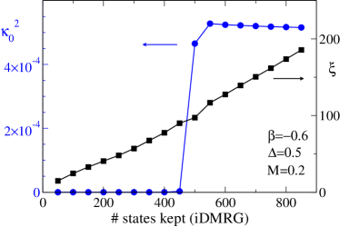
Figure 6: (Color online) Convergence of the iDMRG method at the point $\beta=-0.6$, $\Delta=0.5$, $M=0.2$. The largest intrinsic correlation length $\xi$ of the matrix-product iDMRG methodiDMRG and square of the chirality $\kappa_{0}^{2}$ are shown as functions of the number of states kept in the iDMRG calculation.

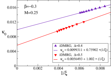
Figure 7: (Color online) An example of extrapolation in the inverse correlation length $\xi$ for the chiral order parameter $\kappa_{0}$, at $\beta=-0.3$ and $M=0.25$, for two anisotropies $\Delta=0.4$ and $\Delta=0.5$ where $\kappa_{0}$ becomes very small, cf. Fig. 5(b). Up to $m=1000$ steps were kept in those iDMRG calculations.

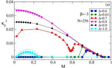
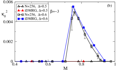
Figure 8: (Color online) Square of the vector chirality $\kappa_{0}^{2}$ at $\beta=-3$ as a function of the magnetization $M$ at several values of the anisotropy $\Delta$: (a) finite-size DMRG results for a system of $N=256$ spins; (b) comparison of the finite-size DMRG and iDMRG results for paths crossing the chiral phase boundary.

III.3 Vector chirality in the strong coupling regime ($|J_{1}|>J_{2}$)

The behavior of the chiral order parameter in the regime of strong coupling $\beta=-3$, as extracted from the finite-size DMRG and iDMRG calculations, is shown in Fig. 8. It indicates the existence of a chiral phase that is contained inside a relatively narrow stripe $0.5<\Delta<1$, and the rest of the $\Delta S^{z}=1$ region should belong to a non-chiral spin-fluid phase. The presence of a kink in the magnetization curves further suggests that this spin-fluid phase is in turn divided into the one-component (TL1) and two-component (TL2) spin fluid phases, occupying the low- and high-field regions, respectively.

As can be seen from Fig. 8(a), the transition between the chiral phase and the TL1 phase is very sharp: the chiral order drops from a sizeable value to zero in the entire low-field region, when the anisotropy changes from $\Delta=0.7$ to $\Delta=0.65$. This suggests that the transition is of the first order.

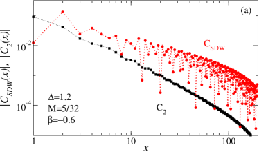
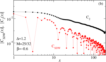
Figure 9: (Color online) Comparison of the nematic correlator $C_{2}(x)$ and the spin density wave correlator $C_{\rm SDW}(x)$, defined by Eqs. (4), (5), respectively, as a function of distance $x=|n-n^{\prime}|$, at $\beta=-0.6$ and two different magnetizations: (a) $M=5/32$; (b) $M=25/32$. Here, finite-size DMRG results for a system of $N=256$ spins are shown.

Figure 8(b) illustrates that for $\beta=-3$, the iDMRG results agree very well with the finite-size DMRG data for a $256$-spin chain. This fact, together with the abrupt character of the transition from the chiral phase to the TL1 spin fluid, gives us reasons to conclude that in the strong coupling case the observation of non-chiral regions is not an artefact of the DMRG convergence, but is due to existence of spin-fluid phases, in contrast to the behavior in the weak coupling regime $|\beta|<1$.

III.4 Crossover between the spin density wave and nematic at $\beta=-0.6$

We have analyzed the crossover between $\rm SDW_{2}$ and nematic correlations inside the quadrupolar $\Delta S^{z}=2$ phase at $\beta=-0.6$. The typical behavior of the SDW and nematic correlations as defined by Eqs. (4), (5) is shown in Fig. 9. One can see that both correlators decay as power law, but the SDW correlations dominate in the low-field region, while the nematic correlations take over at high magnetizations, in agreement with the bosonization analysis and earlier numerical results.hm06a ; vekua07 ; kecke07 The effect of the anisotropy $\Delta$ on this crossover is rather mild: an easy-plane anisotropy $\Delta<1$ shifts the crossover boundary towards higher $M$, making the nematic region more narrow, and the crossover boundary seems to be insensitive to an easy-axis anisotropy $\Delta>1$.

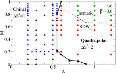
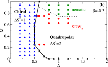
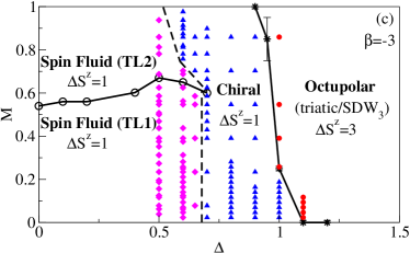
Figure 10: (Color online) Phase diagrams of the Hamiltonian (I), represented as slices in the space of the magnetization $M$ and anisotropy $\Delta$, at fixed frustration $\beta=J_{1}/J_{2}$: (a) at $\beta=-0.6$; (b) $\beta=-0.3$; (c) $\beta=-3$. Solid lines denote phase boundaries (extrapolated in $1/N$) as extracted from $M(h)$. Dashed lines denote the approximate phase boundaries as extracted from the correlations analysis, and dotted lines in (a) and (b) denote the position of a crossover between the dominant spin-density wave (SDW) and nematic correlations. Solid symbols result from the analysis of correlations functions: Triangles (blue) correspond to the points in a chirally ordered phase, diamonds (magenta) to the one- and two-component spin-fluid (TL1 and TL2, respectively); at $\beta=-0.3$ and $\beta=-0.6$, circles (red) denote points with dominant $\rm SDW_{2}$ correlations, and squares (green) indicate points with dominant nematic correlations within the quadrupolar ($\Delta S^{z}=2$) phase. At $\beta=-3$, circles (red) denote points in the octupolar ($\Delta S^{z}=3$) phase without specifying the dominant type of correlations ($\rm SDW_{3}$ or triatic).

IV Magnetic phase diagrams

Summarizing all the information extracted from the analysis of magnetization curves and correlations, one can establish the phase diagrams of the anisotropic frustrated ferromagnetic spin-$\frac{1}{2}$ chains in the presence of a magnetic field. Such phase diagrams in the $(M,\Delta)$ plane at different values of the frustration $\beta=J_{1}/J_{2}$ are presented in Fig. 10.

We reiterate here that we ascribe the entire $\Delta S^{z}=1$ region to the chiral phase for $\beta=-0.3$ and $\beta=-0.6$, based on the very smooth character of how the order parameter vanishes approaching the $\Delta S^{z}=1$ boundary, on theoretical estimates for zero-field case,furukawa08 and by invoking continuity arguments. In principle, from our data, we cannot exclude the existence of a small non-chiral region in the low-field part of the phase diagram near the $\Delta S^{z}=1$ boundary, but we think that this scenario is rather unlikely. Thus, in the regime of weakly coupled chains, the phase diagram contains just the chiral and quadrupolar phases, the transition between them being likely a smooth (second-order) one.

In the strong coupling regime, $\beta=-3$, our results suggest a rich phase diagram, displaying four phases: the octupolar, the chiral, and two types of spin-fluid phases (which can be characterized as one- and two-component Tomonaga-Luttinger liquids). The transition between the chiral and the spin-fluid-TL1 phase is very sharp and is likely first order.

V Summary

Motivated by recent experimental results for several quasi one-dimensional magnetic materials,hase04 ; enderle05 ; drechsler07 ; banks07 ; Buettgen+07 ; schrettle08 ; banks+09 we studied the model (I) of an anisotropic frustrated ferromagnetic spin-$\frac{1}{2}$ chain in an external magnetic field, at finite values of the magnetization.

We showed that an easy-axis anisotropy $\Delta>1$ stabilizes multipolar phases,vekua07 ; sudan09 ; hikihara08 in which the total $z$-projection of the spin $S^{z}$ increases by steps of $\Delta S^{z}>1$. In the presence of even a small easy-axis anisotropy, such phases occupy the entire range of finite magnetizations up to full saturation. Further, we found that an easy-plane anisotropy $\Delta<1$ may favor several types of phases: chirally ordered and non-chiral one- and two-component spin fluids. We showed that the presence of a moderate easy-plane anisotropy leads to the possibility of a field-induced quantum phase transition at a substantially large value of the magnetization $M$, even in the purely one-dimensional model (I), which might provide an explanation for the field-induced transitionbanks07 ; schrettle08 ; Buettgen+07 from a helically ordered to a collinear state observed in $\rm LiCuVO_{4}$.

Assuming that $\rm LiCuVO_{4}$ is a system of weakly coupled one-dimensional chains and further assuming that the presence of an exchange anisotropy drives the experimentally observed mid-field phase transition in this material, our results imply that the low-field region would be in a helical cone-type phase (see Ref. UedaTotsuka09, for a recent study of helical order in a 3D magnet in high magnetic fields) while the SDW instability in the high-field region would turn the high field region into a collinear, magnetically ordered state with long-range incommensurate $\langle S^{z}(x)S^{z}(0)\rangle$ correlations. The former conclusion (a helical phase in the low-field region) is in agreement with the available experimental data,enderle05 ; banks07 ; schrettle08 while the latter conjecture of collinear incommensurate order could be tested by neutron scattering experiments and is consistent with the nuclear magnetic resonance measurements Buettgen+07 ; schrettle08 suggesting that the magnetic order becomes collinear in applied fields above $\approx 7.5$ T. It should be mentioned that a similar incommensurate collinear structure has been recently observed Kimura+08 in the quasi-1D material $\rm BaCo_{2}V_{2}O_{8}$ with easy-axis anisotropy.

For $\beta=-0.3$, our data suggest that the low-field, chiral region opens up at a finite anisotropy; within the numerical accuracy of our calculations, we were able to resolve the emergence of this region for $\Delta\lesssim 0.8$ [see Fig. 10(b)].

This has to be contrasted against the experimental estimate of the easy-axis anisotropy of about 10%,Vasilev+01 ; KrugVonNidda+02 and against the fact that in the magnetization measurements in $\rm LiCuVO_{4}$, the mid-field transition is observed at $7.5$ T, corresponding to about 20% of the saturation field.banks07 ; enderle05 We stress that our results do not serve to unambiguously prove the exchange anisotropy to be the relevant mechanism behind the mid-field transition in $\rm LiCuVO_{4}$; nevertheless, our results clearly indicate that, using the values for $\beta$ and $\Delta$ suggested for $\rm LiCuVO_{4}$, this material is very close to the quantum critical point at which, as a function of decreasing $\Delta$, a mid-field phase transition develops. This transition point shifts to larger field as the anisotropy increases ($\Delta$ decreases).

The vicinity to many competing phases then makes this material so interesting but also renders it difficult to quantitatively predict its phase diagram. Additional experimental data are highly desirable to clarify the nature of this phase transition, while, in conclusion, our work shows that the emergent physics in this model, driven by the magnetic field, quantum fluctuations and broken exchange symmetry, is very rich.

- (1) J. Villain, Ann. Isr. Phys. Soc. 2, 565 (1978).
- (2) A. F. Andreev and I. A. Grishchuk, Sov. Phys. JETP 60, 267 (1984).
- (3) A. V. Chubukov, Phys. Rev. B 44, 4693 (1991).
- (4) A. K. Kolezhuk and T. Vekua, Phys. Rev. B 72, 094424 (2005).
- (5) A. Läuchli, F. Mila, and K. Penc, Phys. Rev. Lett. 97, 087205 (2006).
- (6) T. Vekua, A. Honecker, H.-J. Mikeska, and F. Heidrich-Meisner, Phys. Rev. B 76, 174420 (2007).
- (7) T. Hikihara, L. Kecke, T. Momoi, and A. Furusaki, Phys. Rev. B 78, 144404 (2008).
- (8) J. Sudan, A. Lüscher, and A. Läuchli, Phys. Rev. B 80, 140402 (2009)
- (9) M. Kaburagi, H. Kawamura, and T. Hikihara, J. Phys. Soc. Jpn. 68, 3185 (1999).
- (10) T. Hikihara, M. Kaburagi, and H. Kawamura, Phys. Rev. B 63, 174430 (2001).
- (11) P. Lecheminant, T. Jolicoeur, and P. Azaria, Phys. Rev. B 63, 174426 (2001).
- (12) A. A. Nersesyan, A. O. Gogolin, and F. H. L. Eßler, Phys. Rev. Lett. 81, 910 (1998).
- (13) A. K. Kolezhuk, Phys. Rev. B 62, R6057 (2000).
- (14) I. P. McCulloch, R. Kube, M. Kurz, A. Kleine, U. Schollwöck, and A. K. Kolezhuk, Phys. Rev. B 77, 094404 (2008).
- (15) K. Okunishi, J. Phys. Soc. Jpn. 77, 114004 (2008).
- (16) F. Heidrich-Meisner, A. Honecker, and T. Vekua, Phys. Rev. B 74, 020403(R) (2006).
- (17) L. Kecke, T. Momoi, and A. Furusaki, Phys. Rev. B 76, 060407(R) (2007).
- (18) K. A. Al-Hassanieh, C. D. Batista, G. Ortiz, and L. N. Bulaevskii, arXiv:0905.4871 (unpublished).
- (19) L. N. Bulaevskii, C. D. Batista, M. V. Mostovoy, and D. I. Khomskii, Phys. Rev. B 78, 024402 (2008).
- (20) H. J. Schulz, Phys. Rev. B 34, 6372 (1986).
- (21) S. R. White and I. Affleck, Phys. Rev. B 54, 9862 (1996).
- (22) D. Allen and D. Sénéchal, Phys. Rev. B 55, 299 (1997).
- (23) C. Itoi and S. Qin, Phys. Rev. B 63, 224423 (2001).
- (24) E. Plekhanov, A. Avella, and F. Mancini, J. Phys.: Conf. Series 145, 012063 (2009); see also arxiv:0811.2973 (unpublished).
- (25) A. Avella, F. Mancini and E. Plekhanov, Eur. Phys. J. B 66, 295 (2008).
- (26) R. D. Somma and A. A. Aligia, Phys. Rev. B 64, 024410 (2001).
- (27) D. V. Dmitriev and V. Y. Krivnov, Phys. Rev. B 77, 024401 (2008).
- (28) D. V. Dmitriev and V. Y. Krivnov, Phys. Rev. B 79, 054421 (2009).
- (29) S. Furukawa, M. Sato, Y. Saiga, and S. Onoda, J. Phys. Soc. Jpn. 77, 123712 (2008).
- (30) M. Enderle, C. Mukherjee, B. Fåk, R. K. Kremer, J.-M. Broto, H. Rosner, S.-L. Drechsler, J. Richter, J. Malek, A. Prokofiev, W. Aßmus, S. Pujol, J.-L. Raggazzoni, H. Rakoto, M. Rheinstädter, and H. M. Rønnow, EPL 70, 237 (2005).
- (31) M. Hase, H. Kuroe, K. Ozawa, O. Suzuki, H. Kitazawa, G. Kido, and T. Sekine, Phys. Rev. B 70, 104426 (2004).
- (32) S.-L. Drechsler, O. Volkova, A. N. Vasiliev, N. Tristan, J. Richter, M. Schmitt, H. Rosner, J. Málek, R. Klingeler, A. A. Zvyagin, and B. Büchner, Phys. Rev. Lett. 98, 077202 (2007).
- (33) M. G. Banks, R. K. Kremer, C. Hoch, A. Simon, B. Ouladdiaf, J.-M. Broto, H. Rakoto, C. Lee, and M.-H. Whangbo, Phys. Rev. B 80, 024404 (2009).
- (34) M. G. Banks, F. Heidrich-Meisner, A. Honecker, H. Rakoto, J.-M. Broto, and R. K. Kremer, J. Phys.: Condensed Matter 19, 145227 (2007).
- (35) F. Schrettle, S. Krohns, P. Lunkenheimer, J. Hemberger, N. Büttgen, H.-A. Krug von Nidda, A. V. Prokofiev, and A. Loidl, Phys. Rev. B 77, 144101 (2008).
- (36) N. Büttgen, H.-A. Krug von Nidda, L. E. Svistov, L. A. Prozorova, A. Prokofiev, and W. Aßmus, Phys. Rev. B 76, 014440 (2007).
- (37) A. N. Vasil’ev, L. A. Ponomarenko, H. Manaka, I. Yamada, M. Isobe, and Y. Ueda, Phys. Rev. B 64, 024419 (2001).
- (38) H.-A. Krug von Nidda, L. E. Svistov, M. V. Eremin, R. M. Eremina, A. Loidl, V. Kataev, A. Validov, A. Prokofiev, and W. Aßmus, Phys. Rev. B 65, 134445 (2002).
- (39) S. R. White, Phys. Rev. Lett. 69, 2863 (1992).
- (40) S. R. White, Phys. Rev. B 48, 10345 (1993).
- (41) U. Schollwöck, Rev. Mod. Phys. 77, 259 (2005).
- (42) K. Okunishi and T. Tonegawa, J. Phys. Soc. Jpn. 72, 479 (2003).
- (43) For the zero-field case, the results of Ref. somma01, imply the antiferromagnetic (“up-up-down-down” type) order for and . We have not attempted to make a connection to these results as our key interest is in the finite magnetization case, where the antiferromagnetic order is already destroyed.
- (44) R. O. Kuzian and S.-L. Drechsler, Phys. Rev. B 75, 024401 (2007).
- (45) K. Okunishi, Y. Hieida, and Y. Akutsu, Phys. Rev. B 60, R6953 (1999).
- (46) I. P. McCulloch, J. Stat. Mech.: Theor. Exp., P10014 (2007).
- (47) I. P. McCulloch, arXiv:0804.2509 (unpublished).
- (48) T. Nishino, K. Okunishi and M. Kikuchi, Phys. Lett. A 213, 69 (1996); L. Tagliacozzo, Thiago R. de Oliveira, S. Iblisdir, and J. I. Latorre, Phys. Rev. B 78, 024410 (2008).
- (49) F. Pollmann, S. Mukerjee, A. Turner, J. E. Moore, Phys. Rev. Lett. 102, 255701 (2009).
- (50) I. P. McCulloch, L. Tagliacozzo and G. Vidal, in preparation.
- (51) The error bars in the finite-size DMRG results for the chiral order parameter in Figs. 5,8 are crude estimates reflecting only the degree of asymptotic “flatness” of the chiral correlators like shown in Fig. 4 (larger error bars imply that there is still a nonzero slope at large distances). Those error bars are thus just the measure of the strength of proliferation of the boundary effects into the bulk, and do not include any uncertainties related to the finite-size effects.
- (52) The reason is that a too small effectively introduces a gap in the symmetric sector, which kills the twist termnersesyan98 and prevents the emergence of chirality.
- (53) H. T. Ueda and K. Totsuka, Phys. Rev. B 80, 014417 (2009).
- (54) S. Kimura, M. Matsuda, T. Masuda, S. Hondo, K. Kaneko, N. Metoki, M. Hagiwara, T. Takeuchi, K. Okunishi, Z. He, K. Kindo, T. Taniyama, and M. Itoh, Phys. Rev. Lett. 101, 207201 (2008).