Tunnel magnetoresistance of magnetic junctions
with cubic symmetry of the layers

Abstract

A tunnel magnetic junction is considered with magnetic hard and magnetic soft layers of cubic symmetry. The magnetic switching is analyzed of the layers by a magnetic field perpendicular to the initial magnetizations. In such a situation, an additional peak of the TMR ratio appears at the magnetic field value lower substantially than the anisotropy energy of the soft layer.

1 Introduction

The tunnel magnetoresistance (TMR) is one of the most important effects in modern spintronics. It attracts interest as a beautiful phenomenon as well as a basis of promising spintronic devices such as magnetic random access memory (MRAM), magnetic sensors, and magnetotunnel transistors (see, e.g., [1, 2]).

Recently, interest has revived to the magnetic junctions with magnetic layers of the cubic-symmetrical materials, such as well-known iron [3, 4, 5]. Thin iron films of (001) orientation have two in-plane easy axes, [100] and [010], with equal anisotropy energy. This fact allows switching magnetization by magnetic field between different easy axes, so that a possibility occurs of creating a memory with more than two stable states, that may be laid to the basis of many-valued logic devices. Moreover, very high TMR ratio, from 170% at room temperature to 318% at 10 K, has been observed in epitaxial Fe/MgO/Fe magnetic tunnel junctions [5] (note, that such high TMR ratios were predicted theoretically [6, 7]). All this makes such structures to be very attractive objects of study.

In this work, we consider a magnetic junction with magnetic hard and magnetic soft layers of iron-type cubic symmetry. Switching such systems by external magnetic field was studied under various relative magnetic configurations of the layers [4, 8]. Here, a different situation is analyzed, when the magnetic field is applied perpendicularly, rather than collinearly, as usual, to the initial collinear magnetization directions of the layers. It is shown, that a new $\Pi$-shaped resistance peak occurs under these conditions at the magnetic field lower substantially than the anisotropy field, while the peak height is lower significantly than the resistance peaks corresponding to the conventional collinear configurations. Therefore, the system in study obeys more than two resistive states switchable by an applied magnetic field.

In Sec. 2 we describe the structure in study and introduce a phenomenological model. In Sec. 3 the layer magnetization directions are calculated as functions of the magnetic field perpendicular to the initial directions. In Sec. 4 the results obtained are used to calculate the corresponding resistances. In Sec. 5 the results are discussed.

2 The model and main equations

Let us consider a magnetic tunnel junction with magnetic hard (1) and magnetic soft (2) layers of iron-type cubic symmetry. The different values of the magnetic anisotropy of the layers may be ensured with larger thickness or pinning of layer 1. The layers have (001) orientation with in-plane easy axes [100] and [010]. The layer magnetization vectors are directed along the [100] easy axis originally, such parallel configuration corresponds to minimal resistance $R_{P}$ of the junction when the current flows perpendicular to the layer planes (CPP mode). Under magnetization switching by applied magnetic field, the junction resistance changes; this is well-known TMR effect.

The conductance of the tunnel junction is [9]

$$G(\chi)=G_{P}\cos^{2}\frac{\chi}{2}+G_{AP}\sin^{2}\frac{\chi}{2},$$ (1)

where $\chi$ is the angle between the layer magnetization vectors, $G_{P}$ and $G_{AP}$ are the conductances corresponding to parallel ($\chi=0^{\circ}$) and antiparallel ($\chi=180^{\circ}$) configurations of the junction, respectively. The angular dependence of the TMR ratio $F(\chi)$ defined as

$$F(\chi)=\frac{R(\chi)-R_{P}}{R_{P}},\quad R(\chi)\equiv\frac{1}{G(\chi)}$$ (2)

takes the form

$$F(\chi)=\frac{f(1-\cos\chi)}{2+f(1+cos\chi)},$$ (3)

where $f=F(180^{\circ})=(R_{AP}-R_{P})/R_{P}$ coincides with the conventional definition of the TMR ratio [10].

To obtain the TMR ratio as a function of the external magnetic field, it is necessary to find the dependence of the $\chi$ angle on the value and direction of the magnetic field.

The magnetization orientation of the magnetic layer is determined with the minimum condition of the magnetic energy, which takes the following form under cubic symmetry [11]:

$$U(\theta)=-MH\cos(\theta-\alpha)+\frac{1}{2}MH_{a}\sin^{2}\theta\cos^{2}\theta,$$ (4)

where $M$ is the saturation magnetization, $H$ is the external magnetic field, $H_{a}$ is the anisotropy field, $\alpha$ and $\theta$ angles determine directions of the external magnetic field and magnetization vector, respectively; the angles are counted off from [100] axis.

Let the magnetic field be applied along [010] axis ($\alpha=90^{\circ}$). The extremum condition $dU(\theta)/d\theta=0$ takes the form

$$[(1-2\sin^{2}\theta)\sin\theta-h]\cos\theta=0,$$ (5)

where $h=H/H_{a}$ is the dimensionless magnetic field.

The roots $\theta=90^{\circ}\equiv\theta_{1}$ and $\theta=-90^{\circ}\equiv\theta_{2}$ of Eq. (5) correspond to two equilibrium positions of the magnetization vector; with $\alpha=90^{\circ}$, the latter state becomes unstable ($d^{2}U(\theta)/d\theta^{2}<0$) at $h>1$.

The other equilibrium states are determined by the cubic equation with respect to $\sin\theta$

$$2\sin^{3}\theta-\sin\theta+h=0.$$ (6)

At $h<\sqrt{6}/9\equiv h_{0}\approx 0.272$, the equation has three real roots, of which only one corresponds to a stable state, namely,

$$\theta=\arcsin\left(\sqrt{\frac{2}{3}}\cos\left(60^{\circ}+\frac{1}{3}\arccos\frac{h}{h_{0}}\right)\right)\equiv\theta_{3}.$$ (7)

At $h>h_{0}$, the stable solution $\theta_{3}$ disappears (the only real root of Eq. (6) corresponds to an unstable state), and only $\theta_{1}=90^{\circ}$ and $\theta_{2}=-90^{\circ}$ stable states remain.

These results are used below to analyze magnetic configuration of the magnetic junction.

3 Layer magnetization direction

Let us trace behavior of the magnetization vector of a magnetic layer oriented originally along [100] easy axis in the magnetic field directed along another easy axis [010]. With the field increasing from zero, the magnetization vector deflects gradually from the former easy axis to the latter one in accordance with Eq. (7), until $h$ reaches $h_{0}$ value (the corresponding value of $\theta$ angle is $\theta=\arcsin(1/\sqrt{6})\approx 24^{\circ}$) and $\theta_{3}$ state disappears. Then the vector turns abruptly to $\theta_{1}$ position (along the magnetic field and [010] easy axis) and remains in this state with further increase of the magnetic field. It remains in that state, also, when the magnetic field decreases to zero and further to negative value $h=-1$. Then the magnetization vector switches abruptly from the $\theta_{1}$ position antiparallel to the magnetic field to the parallel one $\theta_{2}$ position. Under subsequent cycling of the magnetic field between $h=-1$ and $h=+1$ values, the magnetization switches abruptly between $\theta_{1}$ and $\theta_{2}$ states without returning to the initial state $\theta=0^{\circ}$. The return may be realized by the magnetic field $h=h_{0}$ along [100] axis.

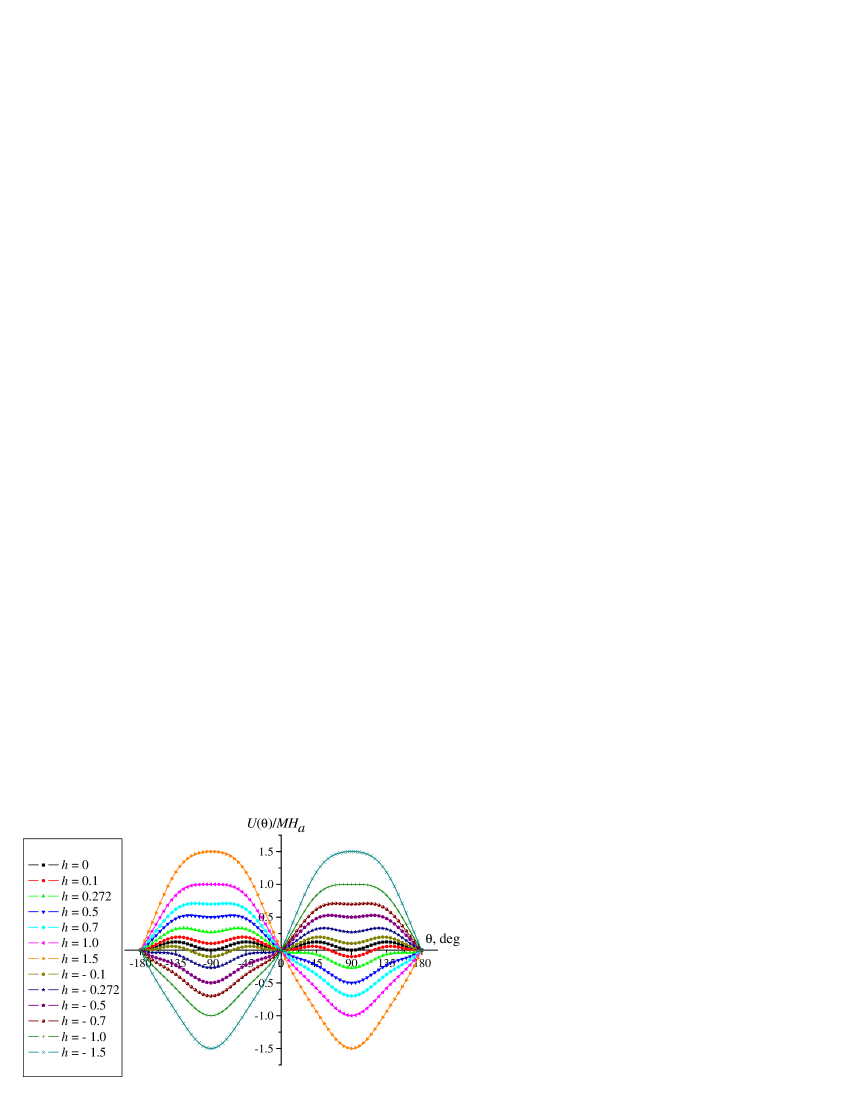
Figure 1: The (dimensionless) magnetic energy of a magnetic layer with cubic symmetry as a function of $\theta$ angle between the magnetization vector and the easy axis at various dimensionless magnetic fields $h=H/H_{a}$ directed along [010] axis ($\theta=90^{\circ}$). The minimum $\theta=0^{\circ}$ disappears at $h=0.272$ so that the system being in that minimum comes to another minimum $\theta=90^{\circ}$. The latter exists under subsequent field changes until $h=-1$, when the system switches to $\theta=-90^{\circ}$ minimum. Under subsequent cycling the magnetic field between $h=-1$ and $h=1$, the system switches between $\theta=-90^{\circ}$ and $\theta=90^{\circ}$ positions without returning to the initial $\theta=0^{\circ}$ position.

Such a behavior of the system with transitions from one energy minimum to another one may be traced also by means of Fig. 1 where the magnetic energy $U(\theta)$ is shown in various magnetic fields.

Now we consider the magnetic junction described in Sec. 2 instead of a single magnetic layer. The each of two layers behaves independently of the other, so that the magnetization direction dependence on the applied magnetic field is to be found as above for both layers, but with different anisotropy energies. We assume, as an example, that the anisotropy energy of the magnetic hard layer is twice as many as that of the soft layer.

Because of larger anisotropy energy, the hard layer lags behind the soft one and switches from one position to another at larger magnetic field. The results are shown in Fig. 2. Three subsequent stages of the whole switching cycle, $0^{\circ}\to 90^{\circ}$, $90^{\circ}\to-90^{\circ}$, and $-90^{\circ}\to 90^{\circ}$, are marked with Roman numerals I, II and III, respectively, the Arabic numerals 1 and 2 refer to the hard and soft layers, respectively.

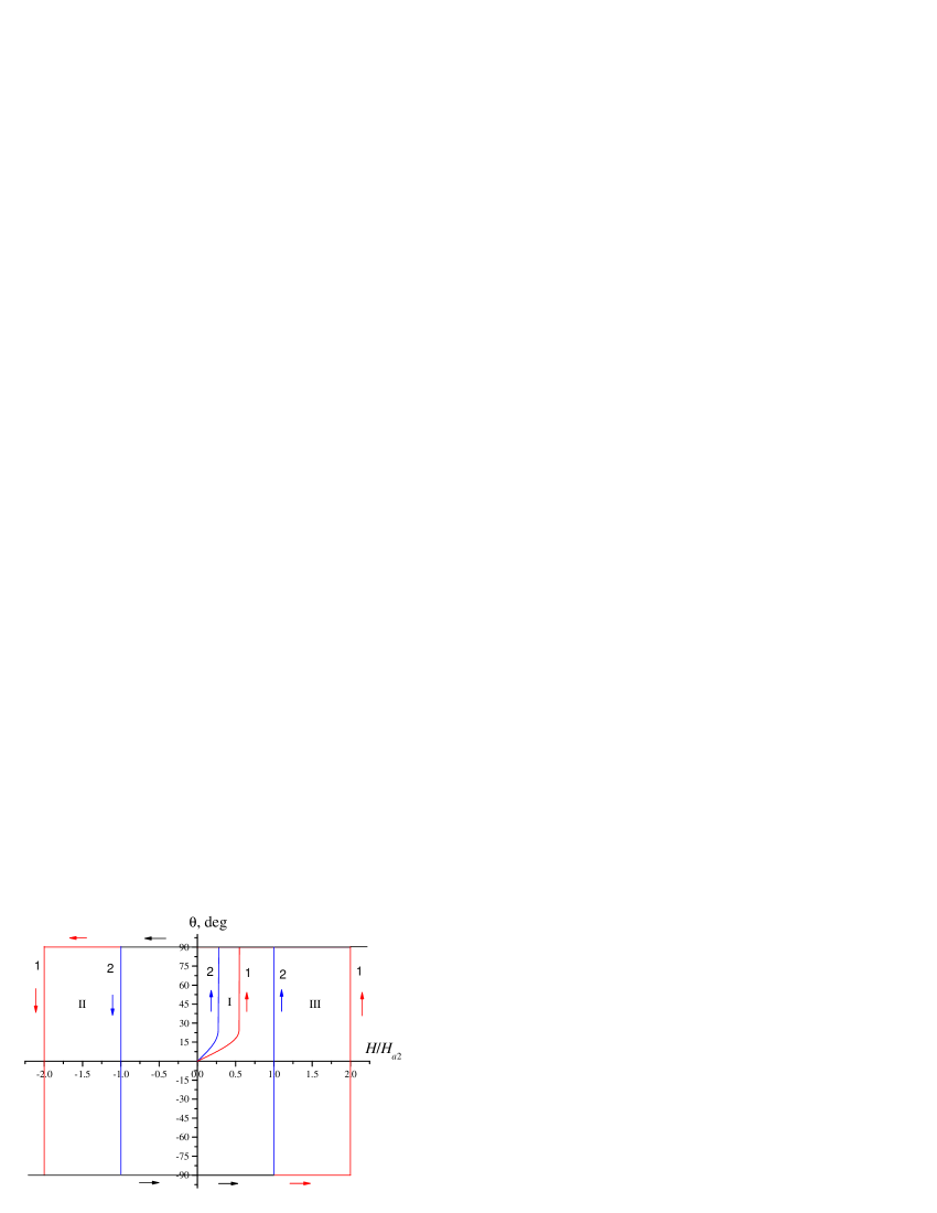
Figure 2: The dependence of the magnetic hard (1) and soft (2) layer orientations on the magnetic field along [010] axis ($\theta=90^{\circ}$) referred to the soft layer anisotropy field $H_{a2}$. The layer anisotropy field ratio $H_{a1}/H_{a2}$ is supposed to be equal to 2, as example. Three subsequent stages of the whole switching cycle, $0^{\circ}\to 90^{\circ}$, $90^{\circ}\to-90^{\circ}$, and $-90^{\circ}\to 90^{\circ}$, are marked with Roman numerals I, II and III, respectively. The arrows show directions of the layer magnetization switching.

4 Tunnel magnetoresistance

The TMR ratio is determined with the difference $\chi$ of the corresponding $\theta$ angles for two layers in accordance with Eq. (3). Using Eqs. (3), (7), we obtain the results shown in Fig. 3. The Roman numerals have the same meaning as in Fig. 2. It is seen, that a new peak I appears besides the standard TMR ratio peaks II and III corresponding to the switching from parallel configuration to antiparallel one and vise versa. This new peak is lower substantially because it corresponds to the angle between the layer magnetization vectors smaller than $90^{\circ}$ (this angle tends to $90^{\circ}$ when the hard layer anisotropy energy is large in comparison with that of the soft layer; in that case, the TMR ratio is half of the standard value). This peak corresponds to the magnetic field value lower considerably (almost 4 times) than the soft layer anisotropy field.

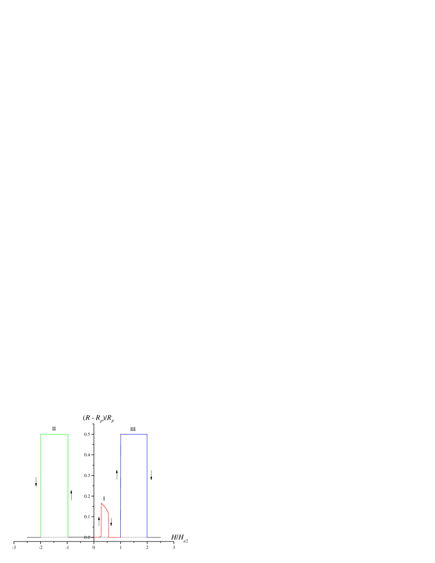
Figure 3: The TMR ratio as a function of the magnetic field along [010] axis ($\theta=90^{\circ}$) referred to the soft layer anisotropy field $H_{a2}$ at $H_{a1}/H_{a2}=2$, $(R_{AP}-R_{P})/R_{P}=0.5$. The Roman numerals and the arrows have the same meaning as in Fig. 2.

5 Conclusion

It follows from the results that using magnetic junctions with cubic rather than uniaxial symmetry of the layers opens additional possibilities in applications of the TMR effect. The switching with a perpendicular magnetic field allows to lower significantly the corresponding magnetic field, that may improve sensibility of the magnetic sensors based on TMR. The extra peak of the TMR ratio as a function of the applied magnetic field means existence of an additional stable equilibrium state of the system in study. This fact may be used to create memory devices with more than two stable states and multi-valued logic devices.

References

- [1] G.A. Prinz, J. Magn. Magn. Mater. 200, 57 (1999)
- [2] A. Fert, Rev. Mod. Phys. 80, 1517 (2008)
- [3] J. Grabowski, M. Przybylski, M. Nyvlt, J. Kirschner, J. Appl. Phys. 104, 113905 (2008)
- [4] R. Lehndorff, M. Buchmeier, D.E. Bürger, A. Kakay, R. Hertel, C.M. Schneider, Phys. Rev. B 76, 214420 (2007)
- [5] S.G. Wang, R.C.C. Ward, G.X. Du, X.F. Han, C. Wang, A. Kohn, Phys. Rev. B 78, 180411 (2008)
- [6] W.H. Butler, X.-G. Zhang, T.C. Schulthess, J.M. MacLaren, Phys. Rev. B 63, 054416 (2001)
- [7] J. Mathon, A.Umerski, Phys. Rev. B 63, 220403 (2001)
- [8] A.A. Leonov, U.K. Rößler, A.N. Bogdanov, J. Appl. Phys. 104, 084304 (2008)
- [9] Y. Utsumi, Y. Shimizu, H. Miyazaki, J. Phys. Soc. Japan 68, 3444 (1999)
- [10] M. Guilliere, Phys. Lett. A 54, 225 (1975)
- [11] K.H.J. Buschow, F.R. De Boer, Physics of Magnetism and Magnetic Materials (Kluwer Academic Publ., New York, 2003)